An integrated model of soil-canopy spectral radiance observations, photosynthesis, fluorescence, temperature and energy balance

(1)

BGD

6, 6025–6075, 2009

An integrated model of soil-canopy spectral radiance

observations

C. van der Tol et al.

Title Page

Abstract Introduction

Conclusions References

Tables Figures

◭ ◮

Back Close

Full Screen / Esc

Printer-friendly Version

Interactive Discussion

Biogeosciences Discuss., 6, 6025–6075, 2009 www.biogeosciences-discuss.net/6/6025/2009/ © Author(s) 2009. This work is distributed under the Creative Commons Attribution 3.0 License.

Biogeosciences Discussions

Biogeosciences Discussionsis the access reviewed discussion forum ofBiogeosciences

An integrated model of soil-canopy

spectral radiance observations,

photosynthesis, fluorescence,

temperature and energy balance

C. van der Tol1, W. Verhoef1, J. Timmermans1, A. Verhoef2, and Z. Su1

1

ITC International Institute for Geo-Information Science and Earth Observations, Hengelosestraat 99, P.O. Box 6, 7500 AA, Enschede, The Netherlands

2

Dept. of Soil Science, The University of Reading, Whiteknights, Reading, RG6 6DW, UK

Received: 20 May 2009 – Accepted: 25 May 2009 – Published: 23 June 2009

Correspondence to: C. van der Tol (tol@itc.nl)

(2)

BGD

6, 6025–6075, 2009

observations

Title Page

Tables Figures

◭ ◮

Back Close

Full Screen / Esc

Interactive Discussion Abstract

This paper presents the model SCOPE (Soil Canopy Observation, Photochemistry and Energy fluxes), which is a vertical (1-D) integrated radiative transfer and energy balance model. It calculates the radiation and the energy balance of a vegetated land surface at the level of single leaves as well as at canopy level, and the spectrum of

5

the outgoing radiation in the viewing direction, at a high spectral resolution over the

range from 0.4 to 50µm, thus including the visible, near and shortwave infrared, as

well as the thermal domain. A special routine is dedicated to the calculation of chloro-phyll fluorescence. The calculation of radiative transfer and the energy balance is fully integrated, allowing for feedback between surface temperatures, leaf chlorophyll

fluo-10

rescence and radiative fluxes. Model simulations were evaluated against observations reported in the literature. The model may serve as a theoretical ground truth to derive relationships between observed spectra and physical processes at the land surface.

1 Introduction

Knowledge of physical processes at the land surface are relevant for a wide range of

15

applications including weather and climate prediction, agriculture, and ecological and hydrological studies. Of particular importance are the fluxes of energy, carbon dioxide and water vapour between land and atmosphere.

During the last decades scientific understanding of physical processes at the land surface has grown, as a result of the increased availability of data, both from ground

20

based and remote sensors. The implementation of a network of flux towers (FLUXNET)

has increased the knowledge about processes at plot level in diff_{erent ecosystems and}

diff_{erent climates (Baldocchi, 2003). This knowledge has been widely incorporated in}

detailed coupled models for energy, carbon dioxide and water transport between soil, vegetation and atmosphere (e.g. Sellers et al., 1997; Verhoef and Allen, 2000; Tuzet et

25

al., 2003).

(3)

BGD

6, 6025–6075, 2009

observations

Title Page

Tables Figures

◭ ◮

Back Close

Full Screen / Esc

Data from high resolution optical imagers, multi-spectral radiometers and radar on satellite platforms are nowadays available to retrieve spatial information about topogra-phy, soil and vegetation (CEOS, 2008). For example, Verhoef and Bach (2003) derived vegetation parameters by inverting a radiative transfer model. Attempts have also been made to estimate evaporation from thermal images (Bastiaanssen, 1998).

Further-5

more, remote sensing (RS) data have been used as input for spatial soil-vegetation-atmosphere-transfer (SVAT) models for estimation of the surface energy balance (Kus-tas et al., 1994; Su, 2002; Anderson et al., 2008).

The potential of remote sensors operating at diff_{erent spatial, temporal and spectral}

resolution is not yet fully exploited, for various reasons. First, remote sensing data is

10

often of too coarse spatial resolution for SVAT models, which are detailed and require field-scale data (Hall et al., 1992). Second, the variables derived from remote sensing

are diff_{erent from those required by a SVAT model. A variable retrieved from remote}

sensing (such as leaf area index) may have a diff_{erent meaning than a variable with}

the same name used in a SVAT model (Norman and Becker, 1995).

15

In order to make eff_{ective use of the available RS data, coherent models are needed}

for the interpretation of observed radiance spectra with respect to physical processes on the ground. These models should incorporate fluxes of water, carbon and energy at the land surface, as well as radiative transfer. The model CUPID (Norman, 1979; Kus-tas et al., 2007) has, to our knowledge, been the first model for both radiative transfer

20

and heat, water (vapour) and CO2exchange in canopies. With this model, directional

brightness temperature can be calculated for multiple-source canopies where leaves

and soil have diff_{erent temperatures. The model calculates directional radiance and}

energy fluxes in forward mode, which means that for the interpretation of observed spectra, the model has to be inverted.

25

(4)

BGD

6, 6025–6075, 2009

observations

Title Page

Tables Figures

◭ ◮

Back Close

Full Screen / Esc

spectrum of the outgoing radiance in the viewing direction at a high spectral

resolu-tion over the range from 0.4 to 50µm, thus including the visible, near and shortwave

infrared, as well as the thermal domain. The model calculates the energy balance of the surface (unlike CUPID, the water balance is not calculated). Radiative transfer is

described on the basis of the four-stream SAIL extinction and scattering coeffi_cients

5

(Verhoef, 1984), but the solution method of SCOPE is of a more numerical nature to allow for a heterogeneous vertical temperature distribution.

The purpose of SCOPE is to facilitate better use of remote sensing data in modelling of water and energy fluxes at the land surface. SCOPE can support the interpretation of earth observation data in meteorological, hydrological, agricultural and ecological

10

applications. The calculation of a broad electromagnetic spectrum (0.4 to 50µm)

al-lows for the simultaneous use of diff_{erent sensors for validation. The model can be}

used at the plot scale as a theoretical “ground truth” for testing simpler models, and as such to evaluate relationships between surface characteristics and (parts of) the reflected spectral radiation, such as the relation between indices (e.g. NDVI) and other

15

vegetation characteristics (e.g. LAI). Because it is a 1-D vertical model which assumes homogeneity in horizontal direction, the model may not be applicable for heteroge-neous areas.

The aim of this paper is to describe the model structure and technical and imple-mentation aspects. Examples of model output are compared to the literature, and the

20

potential applications of the model are discussed. A validation of the model against field experiments will be presented in a following paper.

2 Model description 2.1 Model structure

The model SCOPE is based on existing theory of radiative transfer,

micrometeorol-25

ogy and plant physiology. The strength of the model is the way in which interactions

(5)

BGD

6, 6025–6075, 2009

observations

Title Page

Tables Figures

◭ ◮

Back Close

Full Screen / Esc

between the diff_{erent model components are modelled. Three unique features of the}

model make it particularly relevant for future applications:

1. the use of the model PROSPECT (Jacquemoud and Baret, 1990) for optical prop-erties of leaves in combination with a photosynthesis model;

2. the calculation of heterogeneous canopy and soil temperatures in combination

5

with the energy balance;

3. the calculation of chlorophyll fluorescence as a function of irradiance, canopy tem-perature and other environmental conditions.

The model consists of a structured cascade of separate modules. These modules can be used stand alone, or, as in the integrated model, they can be connected by

10

exchanging input and output. Depending on the application, some modules can be left out or replaced by others.

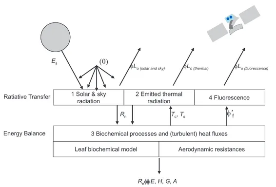
Figure 1 shows schematically how the main modules interact. The model distin-guishes between modules for radiative transfer (of incident light, and internally gen-erated thermal radiation and chlorophyll fluorescence), and the energy balance. The

15

numbers in the figure refer to the order in which they are executed:

1. Semi-analytical radiative transfer module for incident solar and sky radiation, based on SAIL (Verhoef and Bach, 2007): calculates the TOC (top of canopy)

incident radiation spectrum (0.4 to 50µm), as well as the net radiation and

ab-sorbed photosynthetically active radiation (PAR) per surface element.

20

2. Numerical radiative transfer module for thermal radiation generated internally by soil and vegetation, based on Verhoef et al. (2007): calculates the TOC outgoing thermal radiation and net radiation per surface element, for heterogeneous leaf and soil temperatures.

3. Energy balance module for latent, sensible and soil heat flux per surface element,

25

(6)

BGD

6, 6025–6075, 2009

observations

Title Page

Tables Figures

◭ ◮

Back Close

Full Screen / Esc

4. Radiative transfer module for chlorophyll fluorescence based on the FluorSAIL model (Miller et al., 2005): calculates the TOC radiance spectrum of fluorescence from leaf level chlorophyll fluorescence (calculated in step 3) and the geometry of the canopy.

Iteration between modules (2) and (3) is carried out to match the input of the

radia-5

tive transfer model with the output of the energy balance model (skin temperatures), and vice versa: the input of the energy balance model with the output of the radiative

transfer model (net radiation). For computational effi_{ciency, the radiative transfer of}

chlorophyll fluorescence is carried out at the end of the cascade, which implies that the contribution of chlorophyll fluorescence to the energy balance is neglected. Its

con-10

tribution to the outgoing radiance spectrum is finally added to the reflectance. Note that this only holds for the radiative transfer and the calculation of the TOC spectrum of chlorophyll fluorescence (step 4), which is computationally demanding. The chloro-phyll fluorescence at leaf level is calculated every iteration step as a by-product of the photosynthesis model (step 3).

15

The radiative transfer modules serve two purposes: first, to predict the TOC radi-ance spectrum in the observation direction, and second, to predict the distribution of irradiance and net radiation over surface elements (leaves and the soil). The latter is input for the energy balance module. The energy balance module serves two purposes as well: first to calculate the fate of net radiation (i.e. the turbulent energy fluxes and

20

photosynthesis), and secondly to calculate surface temperature and fluorescence of the elements of the surface. The latter are input for the radiative transfer model. Shar-ing input, output and parameters makes it possible to study the relationship between TOC spectra and energy fluxes in a consistent way. For example, the energy balance is preserved at all times (except for the small contribution of chlorophyll fluorescence).

25

For the calculation of radiative transfer, the description of the geometry of the vege-tation is of crucial importance. Leaves and soil are divided into classes which receive a similar irradiance. These classes are the elements of the model. This distinction

of elements is a stochastic technique to describe the eff_{ects of the geometry of the}

(7)

BGD

6, 6025–6075, 2009

observations

Title Page

Tables Figures

◭ ◮

Back Close

Full Screen / Esc

vegetation on the outgoing spectrum and on the heterogeneity of net radiation.

The geometry of the canopy is described as follows. It is assumed that the canopy has a homogeneous structure, and is 1-D only, which means that variations of macro-scopic properties in the horizontal plane are neglected. For the purpose of numerical radiative transfer calculations, 60 elementary layers, with a maximum LAI of 0.1 are

5

defined, so that numerical approximations to the radiative transfer equations are still acceptable up to a total canopy LAI of 6. For the description of canopy architecture, the same as the one used in the SAIL models (Verhoef, 1984, 1998) is applied, which requires a total LAI, two parameters describing the leaf angle distribution and the hot spot parameter. Numerically, 13 discrete leaf inclinations are used as in SAIL, and

10

the uniform leaf azimuth distribution is now also discretised to 36 angles of 5, 15, ... , 355 degrees relative to solar azimuth.

The elements of the model are defined as follows. For shaded leaves, 60 elements are distinguished (corresponding to the 60 leaf layers), since for the assumed

semi-isotropic diff_{use incident fluxes the leaf orientation is immaterial for the amount of flux}

15

that is intercepted. For sunlit leaves, 60_×13_×36 elements (60 leaf layers, 13 leaf

incli-nations,θℓ, and 36 leaf azimuth angles,ϕℓ) are distinguished, since the interception

of solar flux depends on the orientation of the leaf with respect to the sun. The soil is divided into two elements: a shaded and a sunlit fraction.

In the model, the principle of linearity of the radiative transfer equation is exploited by

20

combining the solutions for various standard boundary conditions and source functions, such as the ones related to the optical domain, the thermal domain, and the ones related to direct solar radiation, sky radiation, leaves in the sun, and leaves in the shade. The latter distinction is particularly important for the biochemistry components

of the model (photosynthesis and fluorescence). Calculations for diff_{erent parts of the}

25

spectrum, sources of radiation, and elements of the surface are carried out separately,

and total fluxes are obtained afterwards by adding the diff_{erent contributions. This}

makes it possible to separate the calculation of chlorophyll fluorescence, optical and

(8)

BGD

6, 6025–6075, 2009

observations

Title Page

Tables Figures

◭ ◮

Back Close

Full Screen / Esc

violating energy conservation. This principle is exploited at several places in the model

to enhance the computational effi_{ciency and to create a transparent code.}

In the following sections, the model is described in more detail. The modules are presented in an order which facilitates the conceptual understanding of the model, which is with very few exceptions also the order in which they are executed by the

5

model (Fig. 1). We shall start with a description of the input at the top of the canopy (Sect. 2.2), followed by the radiative transfer models (Sect. 2.3 and 2.4), the calculation of net radiation (Sect. 2.5), the energy balance (Sect. 2.6), leaf biochemical processes (Sect. 2.7), and top-of -canopy outgoing radiance (Sect. 2.8).

2.2 Atmospheric optical inputs 10

The model SCOPE requires top-of-canopy incident radiation as input, at a spectral res-olution high enough to take the atmospheric absorption bands properly into account. For the top of the canopy the incident fluxes from the sun and the sky can be obtained from the atmospheric radiative transfer model MODTRAN (Berk et al., 2000). The cal-culation of TOC incident fluxes is ideally done with MODTRAN before each simulation

15

with SCOPE, using the actual values of solar zenith and azimuth angle and atmo-spheric conditions. An alternative is to create a library of incoming spectra, from which SCOPE can extract a typical spectrum for specific conditions. In this study, only one example spectrum was created with MODTRAN. The shape of this example spectrum is used throughout the paper, while the magnitudes of the optical and thermal part of

20

the spectrum are each linearly scaled according to local broadband measurements of incident irradiance.

From MODTRAN the following outputs are needed:

TRAN=_{direct transmittance from target to sensor}

SFEM=_{radiance contribution due to thermal surface emission}

25

GSUN=_{ground-reflected radiance due to direct solar radiation}

GRFL=_{total ground-reflected radiance contribution}

(9)

BGD

6, 6025–6075, 2009

observations

Title Page

Tables Figures

◭ ◮

Back Close

Full Screen / Esc

spherical albedo, especially at the shorter wavelengths. Two MODTRAN runs, for

sur-face albedos of 50% and 100%, are suffi_{cient to estimate the spherical albedo of the}

atmosphere and the diff_{use and direct solar fluxes incident at the top of the canopy.}

These MODTRAN runs should be done for a low sensor height (1 m above the surface is recommended) under nadir viewing angle, in order to keep the atmospheric

transmit-5

tance from target to sensor as high as possible. With numerical subscripts indicating the surface albedo percentage, all relevant atmospheric and surface quantities can be determined as follows:

ρ_{d d} = GRFL100−2×GRFL50

GRFL₁₀₀₋GRFL₅₀₋SFEM₅₀ (1)

τ_oo =_TRAN ₍₂₎

10

L_s=₂_×_SFEM₅₀_/_TRAN ₍₃₎

O+_T =₍₁₋_ρ_{d d}_)(GRFL₁₀₀₋₂_×_SFEM₅₀₎_/_TRAN ₍₄₎

Esun =π ×GSUN100/TRAN (5)

Here, ρ_{d d} is the spherical albedo of the atmosphere, τ_oo is the direct transmittance

(TRAN) from ground to sensor. Note, that TRAN has no numerical subscript since

15

it is independent of the surface albedo. The double subscripts appended to optical

properties likeρ (reflectance) andτ (transmittance) indicate the types of ingoing and

outgoing fluxes, wheresstands for direct solar flux,d for upward or downward diff_use

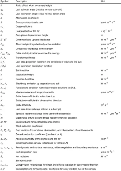
flux andofor flux (radiance) in the observation direction (Verhoef & Bach, 2003). See

also the list of symbols, Table 1. Other symbols in Eqs. (1) to (5) areL_s, the blackbody

20

surface radiance due to thermal emission,E_sun, the solar irradiance on the horizontal

ground surface, and the term O+_T_{, which stands for a certain combination of optical}

and thermal quantities that is independent of the surface albedo. The importance of this term is related to the fact that it can be derived from the MODTRAN outputs and it is required for the estimation of the sky irradiance.

(10)

BGD

6, 6025–6075, 2009

observations

Title Page

Tables Figures

◭ ◮

Back Close

Full Screen / Esc

The sky irradiance onto the surface,Esky, is a derived quantity, which depends partly

on the surface albedo in the surroundings. For arbitrary atmospheric conditions it can be estimated by

Esky =π

_O₊_T

1−aρd d

+_L_s

−Esun , (6)

whereais the surface albedo,

5

O=₍_τ_ss+_τ_sd₎_E_s_(t)_/π

T =_L_a_(b)₋₍₁₋_ρ_{d d}₎_L_s , (7)

and whereEs(t) is the extraterrestrial (TOA) solar irradiance on a plane parallel to the

horizontal plane at ground level,La(b) is the thermal emitted sky radiance at the bottom

of the atmosphere (BOA), assumed to be isotropic. Note that (t) and (b) indicate the

top and the bottom of the atmosphere, respectively. The transmittancesτssandτsd are

10

the direct and the diff_{use transmittances for direct solar flux from TOA to the ground.}

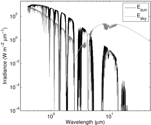
As an example, and to illustrate the broad spectral range involved, Fig. 2 shows the

spectra ofE_sun andE_sky (in W m−2µm−1) for a surface albedo of zero. From these

re-sults it can be concluded that at 2.5µm already the diff_{use sky irradiance starts to rise}

due to thermal emission, and at wavelengths longer than 8µm it is the dominant source

15

of incident radiation. In spectral regions of low atmospheric absorption (high transmit-tance) the thermal sky radiance is less than in absorption bands. This is caused by the correspondingly lower atmospheric emissivity and the fact that higher and thus colder layers of the atmosphere contribute to the radiance at surface level.

Note that Eqs. (5) and (6) are used to calculate the atmospheric spectral inputs of

20

SCOPE, but they are not part of the model code itself.

2.3 Direct and di_ffuse fluxes

In the first radiative transfer module of SCOPE, the eff_{ects of thermal emission by}

surface elements are ignored and in this case the analytical solutions for the diff_use

(11)

BGD

6, 6025–6075, 2009

observations

Title Page

Tables Figures

◭ ◮

Back Close

Full Screen / Esc

and direct fluxes as obtained from the SAIL model are used to calculate the vertical profiles of these fluxes inside the canopy layer. In addition, net radiation and absorbed PAR are calculated for soil and leaf elements.

For the diff_{use upward (}_E+_{) and downward (}_E−_{) fluxes (W m}−2_µ_m−1_{), use is made}

of numerically stable analytical solutions as provided in the more recent 4SAIL model

5

(Verhoef et al., 2007). This is further explained in Appendix A. The direct solar flux is described by

Es(x)=Es(0)Ps(x) (8)

whereEs(0) is the direct solar flux incident at the top of the canopy (Esun), andPs(x) is

the probability of leaves or soil being sunlit (or the gap fraction in the solar direction),

10

which is given by P_s(x)=_exp(₋_kLx_{), where} _x _{is the relative optical height ([}₋_{1, 0],}

where –1 is at the soil surface and 0 at TOC),Lis the leaf area index (LAI), and k is

the extinction coeffi_{cient in the direction of the sun. As shown in Appendix A, the di}ff_use

upward and downward fluxes are derived from transformed fluxesF1andF2, which are

given by

15

F1(x)=δ1e

mLx₊

(s′+_r

∞s)Es(0)J1(k, x)

F2(x)=δ2e−

mL(1+_x)₊

(r_∞s′+_s₎_E_s₍₀₎_J₂₍_{k, x}₎

(9)

where m is the eigenvalue of the diff_{use flux system,} _r

∞ is the infinite reflectance

(i.e. the bi-hemispherical reflectance for infinite LAI),s the backscatter coeffi_cient, _s_′

the forward scatter coeffi_cient,_J₁_and_J₂_{numerically safe functions as described in}

Ver-hoef and Bach (2007), andδ1and δ2 are boundary constants. In Appendix A, more

20

extensive information is given about the SAIL coeffi_{cients, their use in the analytical}

so-lution, the boundary constants for given solar and sky irradiance, and the incorporation of the soil’s reflectance.

The coeffi_cients _m_, _s_, _s_′ _and _r

∞ in Eq. (9) depend on the transmittance and

re-flectance of the leaves and the leaf inclination distribution. The spectral transmittance

25

(12)

BGD

6, 6025–6075, 2009

observations

Title Page

Tables Figures

◭ ◮

Back Close

Full Screen / Esc

and Baret, 1990), using the concentrations of leaf water, chlorophyll, dry matter, and

brown pigment, as well as the leaf mesophyll scattering parameterN, as input

parame-ters. The soil’s reflectance spectrum is another required input. In this study, a standard spectrum for a loamy sand soil was used.

2.4 Internally generated thermal radiation 5

The incident radiation on leaves should not only include the optical and thermal radi-ation from sun and sky, but also all thermal radiradi-ation that is generated internally by leaves and by the soil. In Verhoef et al. (2007) the thermal domain was treated by means of an analytical solution, which assumed distinct, but otherwise constant, tem-peratures of sunlit and shaded leaves, as well as sunlit and shaded soil. However, one

10

may expect that in reality sunlit leaves will all have diff_{erent temperatures, depending on}

their orientation with respect to the sun, and their vertical position in the canopy layer (Timmermans et al., 2008). Therefore, a numerical solution allowing more temperature variation is preferred. For this, the energy balance equation is solved at the level of

individual leaves, for 13_×36 leaf orientations (leaf inclinationθ_ℓ and leaf azimuthϕ_ℓ),

15

and 60 vertical positions in the canopy layer.

In order to compute the internally generated fluxes by thermal emission from leaves and the soil, it is initially assumed that the temperature of the leaves and the soil are equal to the air temperature. Next, the external radiation sources are added, and the energy balance is solved. This gives new temperatures of the leaves and the soil,

20

whereby also sunlit and shaded components are distinguished.

For the numerical solution of this problem, we start with the two-stream diff_erential

equations in which absorption, scattering and thermal emission are included. These are given by

d

LdxE

− ₌_aE−₋_σE+

−εcHc

d

LdxE +

=_σE−₋_aE++_ε_c_H_c (10)

25

whereais the attenuation coeffi_cient,_σ_{the backscatter coe}ffi_cient,_ε_c_{the emissivity of}

(13)

BGD

6, 6025–6075, 2009

observations

Title Page

Tables Figures

◭ ◮

Back Close

Full Screen / Esc

the leaves (canopy), andH_cthe black body emittance. The attenuation coeffi_{cient is the}

diff_{use extinction coe}ffi_cient_κ _{minus the forward scattering coe}ffi_cient_σ′_{, so}_a=_κ₋_σ′_.

This is because forward scattered radiation does not contribute to net attenuation. The

blackbody emittance of the leaves is given byH_c=_πB₍_T_c_{), where}_T_c_{is the vegetation’s}

skin temperature, andBthe Planck blackbody radiance function. Alternatively, radiation

5

integrated over the spectrum can be calculated by using Stefan-Boltzmann’s equation for black body radiation.

The emitted radiation fluxes are calculated at the level of single leaves. In order

to model E− and E+ on the basis of Eq. (10), one needs the emitted radiation at

the level of leaf layers. The layer-level fluxes are calculated by applying a weighted

10

averaging, taking into account the leaf inclination distribution,f(θℓ), and the probability

of sunshine,P_s, in order to diff_{erentiate between leaves in the sun (subscript “}_s_{”) and}

leaves in the shade (subscript “d”):

Hc(x)=Ps(x)

X

13θℓ

36ϕ_ℓ

f(θℓ)Hcs(x, θℓ, ϕℓ)/36+[1−Ps(x)]Hcd(x) (11)

The emittancesH_cs and H_cd are the thermal emitted fluxes from individual leaves in

15

the sun and in the shade, respectively. In order to numerically solve Eq. (10), we use

the corresponding diff_{erential equations for the transformed di}ff_{use fluxes,}_F₁=_E−_r

∞E

+

andF2=−r_∞E−+E

+

, wherer_∞=₍_a₋_m₎_/σ_{. It can be shown that the associated di}ff

er-ential equations for the transformed fluxes are given by:

d

LdxF1=mF1−m(1−r∞)Hc

d

LdxF2=−mF2+m(1−r_∞)Hc

(12)

20

where m=p₍_a2₋_σ2_{) is the eigenvalue of the di}_ff_{use flux system. These di}_ff_erential

(14)

BGD

6, 6025–6075, 2009

observations

Title Page

Tables Figures

◭ ◮

Back Close

Full Screen / Esc

downward and upward directions and that only one independent variable is involved at a time, which leads to a quick convergence.

For the fluxes at the soil level one can write

E+(−1)=_r_s_E−₍₋₁₎+₍₁₋_r_s₎_H_s ₍₁₃₎

wherer_s is the soil’s reflectance andH_s is the black body emittance of the soil.

5

Soil emitted radiation is calculated as a weighted sum of sunlit and shaded soil:

Hs =Ps(−1)Hss +[ 1−Ps(−1)]Hsd (14)

Equations (12, 13) can be used as the basis for a numerical solution of the fluxes in the case of heterogeneous foliage temperatures. An advantage of working with transformed fluxes is that these can be directly expressed in those of the layer above

10

or below the current one, and for a finite diff_{erence numerical solution we obtain the}

simple recursive equations

F1(x−∆x)=(1−mL∆x)F1(x)+m(1−r_∞)Hc(x)L∆x F2(x+ ∆x)=(1−mL∆x)F2(x)+m(1−r∞)Hc(x)L∆x

(15)

If the first transformed flux is given at the canopy top, it can be propagated downwards to the soil level. Next, the second transformed flux can be started at the soil level, and

15

it can be propagated upwards to the top-of-canopy (TOC) level. However, the second transformed flux at the soil level is not known initially, so it has to be derived from the boundary equation, Eq. (13). This gives

F2(−1)=

(r_s₋r_∞)

(1₋r_sr_∞)F1(−1)+

(1₋r_∞2)

(1₋r_sr_∞)(1−rs)Hs (16)

This relation can be used to link the downward and upward sequences of the diff_erence

20

Eq. (15), and finally both transformed fluxes at the TOC level will be available.

The initial guess ofF1(0) is made under the assumption that there is no downward

incident flux at the top of the canopy. Since in the thermal infrared r_∞ is also small,

(15)

BGD

6, 6025–6075, 2009

observations

Title Page

Tables Figures

◭ ◮

Back Close

Full Screen / Esc

we simply assume that initiallyF1(0) is zero. Note that only thermal radiation emitted

by leaves and soil is considered here. Thermal radiation from the sky, which is not negligible, has been treated with the semi-analytical solution described in Sect. 2.3.

After the downward and upward sequences have been completed, also the second

transformed flux at TOC level, F2(0), is known. At this moment one can correct the

5

initial guess ofF1(0), since it was based on the assumption of an upward flux of zero.

For this, use is made of the equation

F1(0)+r_∞F2(0)=(1−r_∞2)E−(0)=0 , (17)

which is rewritten asF1(0)=−r_∞F2(0) .

Summarized, the algorithm works as follows:

10

1. AssumeF1(0)=0

2. Propagate the first line of Eqs. (15) down to the soil level, givingF1(−1)

3. Apply Eq. (16), givingF2(−1)

4. Propagate the second line of Eqs. (15) up to TOC level, givingF2(0)

5. ApplyF1(0)=−r∞F2(0), and go back to step 2, unless the change is less than a

15

given threshold.

In practice, a couple of iterations are usually suffi_{cient to arrive at the correct fluxes at}

both boundaries.

The emissivity parametersεc and εs are input of the model. In this study, uniform

a priori values over the thermal spectrum were used. In future versions of the model,

20

(16)

BGD

6, 6025–6075, 2009

observations

Title Page

Tables Figures

◭ ◮

Back Close

Full Screen / Esc

Interactive Discussion 2.5 Net radiation

Net radiation includes the contributions of all radiation from 0.4 to 50µm. Here, the

principle of linearity of the fluxes is exploited to integrate the energy fluxes, over the spectrum, over the source of radiation and over elements. This implies that the solution obtained from the semi-analytical module for solar and sky radiation (Sect. 2.3) and

5

the solution for internally generated thermal radiation (Sect. 2.4) can be added. Net radiation of a layer is the weighted sum of the contributions from shaded and sunlit

leaves with diff_{erent leaf angles. Similarly, net radiation of the canopy is the sum of the}

contributions of the individual layers.

The net spectral radiation on a leaf is equal to the absorption minus its total emission

10

from the two sides, or, for leaves in the shade

R_n(x)=_[_E−₍_x₎+_E+₍_x₎₋₂_H_cd₍_x_)](1₋_ρ₋_τ₎ ₍₁₈₎

In this equation,E− and E+ are the sum of the externally (solar and sky) and

inter-nally generated fluxes. It is assumed that leaf emissivity ε equals leaf absorptance

α=₁₋_ρ₋_τ_(Kirchhoff_{’s Law), where}_ρ _and_τ_{are the reflectance and the transmittance}

15

of the leaf. For leaves in the sun with a given orientation relative to the sun we obtain

Rn(x, θℓ, ϕℓ)=[|fs|Esun+E−(x)+E

+

(x)₋2Hcs(x, θℓ, ϕℓ)](1−ρ−τ) . (19)

Here,f_s=cosδs

cosθs

=cosθscosθℓ+sinθssinθℓcosϕℓ cosθs ,

whereθ_sis the solar zenith angle and the leaf azimuthϕ_ℓ is taken to be relative with

respect to the solar azimuth.

20

The numerator of the above expression is the projection of the leaf onto a plane perpendicular to the sunrays. Its absolute value is maximal if the leaf’s normal points to the sun or in the opposite direction. The division by the cosine of the solar zenith angle is applied because the solar irradiance is also defined for a horizontal plane. If the leaf’s normal points to the sun, it receives more radiation than a horizontal surface

25

would. The leaf’s emittances (emitted fluxes) are defined for leaves in the shade and

(17)

BGD

6, 6025–6075, 2009

observations

Title Page

Tables Figures

◭ ◮

Back Close

Full Screen / Esc

in the sun. For leaves in the shade the emittance depends only on the vertical position.

Leaves in the sun will all have diff_{erent temperatures and emittances, depending on}

their orientation and vertical position (Sect. 2.4).

2.6 The energy balance

The fate of net radiation is calculated per element with the energy balance model.

5

The energy balance model distributes net radiation over turbulent air fluxes and heat storage.

The energy balance equation for each elementi is given by:

Rn−H −λE −G=0 (20)

whereRn is net radiation, H is sensible andλE is latent heat flux, whereas G is the

10

change in heat storage (all in W m−2). In this equation, energy involved in the melting

of snow and freezing of water is not considered, and energy involved in chemical reac-tions is neglected, since it is usually one or two orders of magnitude smaller than net

radiation. Heat storageGis considered for the soil only (the heat capacity of leaves is

neglected).

15

The turbulent fluxes of an element i are calculated from the vertical gradients of

temperature and humidity for soil (indexk=_{1 in the next equations) or foliage (}_k=_{2) in}

analogy to Ohm’s law for electrical current:

H =_ρ_a_c_pTs−Ta rak

(21)

λE =_λqs(Ts)−qa

r_ak+_r_ck (22)

20

whereρais the air density (kg m−

3

),cpthe heat capacity (J kg−

1

K−1),λthe evaporation

(18)

BGD

6, 6025–6075, 2009

observations

Title Page

Tables Figures

◭ ◮

Back Close

Full Screen / Esc

above the canopy (◦C),q_s the humidity in stomata or soil pores (kg m−3) and q_a the

humidity above the canopy (kg m−3),r_aaerodynamic resistance andr_cstomatal or soil

surface resistance (s m−1). Both H and λE are calculated for each surface element

separately.

Aerodynamic resistancer_a is calculated with the two-source model of Wallace and

5

Verhoef (2000). The model only diff_{erentiates between soil and foliage, and does not}

use separate values for aerodynamic resistance for individual leaf elements. The aero-dynamic model is further explained in Appendix B.

Soil heat flux at the surface G is calculated with the force restore method

(Bhum-rakhar, 1975):

10

∂T_s(t)

∂t = √

2ω

Γ G(t)−ω[Ts(t)−Ts] (23)

whereωis the frequency of the diurnal cycle (radians s−1),Γ_{the thermal inertia of the}

soil (J K−1m−2s−1/2), andTs average annual temperature. The force-restore equation

is discretised to:

T_s(t+ ∆_t₎₋_T_s₍_t₎= √

2ω

Γ ∆tG(t)−ω∆t[Ts(t)−Ts] (24)

15

This equation is used to calculate soil temperature from the temperature at the previous time step. The fact that heat capacity of the soil is not negligible makes it necessary to

simulate a time series of the fluxes in order to obtainG.

The energy balance is closed by adjusting skin temperatures of leaf and soil ele-ments in an iterative manner. It is initially assumed that the skin temperatures of the

20

elements equal the air temperature. After each iteration step, the termsH,λE,Gand

a new estimate of T_s are calculated for each element, using the four energy balance

equations (Eqs. 20, 21, 22 and 24). For numerical stability, a weighted average of the

estimates forT_s of the two previous iteration steps is used in the next iteration step.

It-eration continues until the absolute diff_{erence in net radiation between two consecutive}

25

(19)

BGD

6, 6025–6075, 2009

observations

Title Page

Tables Figures

◭ ◮

Back Close

Full Screen / Esc

Interactive Discussion 2.7 Leaf biochemistry

Leaf biochemistry aff_{ects reflectance, transmittance, transpiration, photosynthesis,}

stomatal resistance and chlorophyll fluorescence. Reflectance and transmittance coef-ficients, which are a function of the chemical composition of the leaf, are calculated with the model PROSPECT (Jacquemoud and Baret, 1990). The other variables not only

5

depend on the chemical composition of the leaf, but also on environmental constraints such as illumination, leaf temperature and air humidity. Their nonlinear responses to environmental constraints are calculated with the model of Van der Tol et al. (2009). This model simultaneously calculates photosynthesis (Farquhar et al., 1980; Collatz et al., 1992), stomatal resistance (Cowan, 1977) and chlorophyll fluorescence. The

flu-10

orescence module is based on conceptual understanding of the relationship between photosystem response and carboxylation. The output is the spectrally integrated level of fluorescence.

In principle, the fluorescence level (W m−2) only needs to be distributed over the

spectrum (W m−2µm−1) in order to obtain the required input for the radiative transfer

15

model: spectrally distributed leaf level fluorescence. However, the matter is compli-cated by two issues. First, the conceptual model is defined at organelle level. At leaf level, re-absorption of fluorescence takes place, which may reduce the fluorescence signal by an order of magnitude (Miller et al., 2005). The re-absorption varies with wavelength and with the thickness and chemical composition of the leaf. Second, the

20

model relies on an a priori value of chlorophyll fluorescence (as a fraction of absorbed PAR) in low light conditions. This a priori value can be obtained from the literature (Genty et al., 1989), but it is unknown whether the value is universal.

To overcome these limitations, the fluorescence level is expressed as a fractionϕ_f′

of that of a leaf in unstressed, low light conditions. This fraction is later (in the radiative

25

(20)

BGD

6, 6025–6075, 2009

observations

Title Page

Tables Figures

◭ ◮

Back Close

Full Screen / Esc

required as input: one for the upper and one for the lower side of a leaf (Sect. 2.8). In future versions of the model, the matrices might be calculated by a model similar to PROSPECT. By using the biochemical model only to describe the response to environ-ment and not the absolute level of chlorophyll fluorescence or its spectral distribution, the problems of re-absorption and parameter estimation are circumvented.

5

Currently, the parameters of the biochemical model may be chosen independently from PROSPECT parameters. The parameters space could be restricted by relating PROSPECT parameters for the optical domain, such as chlorophyll content, to bio-chemical parameters such as photosynthetic capacity. This would make it possible to extract information about photosynthetic capacity from the optical domain.

10

The four most important parameters of the biochemical model are the carboxylation

capacity V_c,max, electron transport capacity Jmax, the dark respiration rate Rd (all in

µmol m−2s−1), and the marginal water cost of photosynthesis λc. The first three

pa-rameters are temperature dependent (accounted for with Arrhenius functions). Various studies have shown that the three parameters are correlated, and usually a constant

15

ratio ofVc,max/Jmax=0.4 is used (Wullschleger, 1993). The parameterVc,maxvaries with

depth in the canopy (Kull and Kruyt, 1998), with day of the year (M ¨akel ¨a et al., 2004) and with plant species (Wullschleger, 1993). Dark respiration and carboxylation ca-pacity both correlate with leaf nitrogen content, but at a global scale, the correlation

coeffi_{cients are low (Reich et al., 1999). The marginal cost of photosynthesis is a}

pa-20

rameter to describe the compromise between the loss of water by transpiration and

uptake of carbon dioxide through stomatal cavities. Parameter λc depends on plant

species and soil water potential. Weak global correlations between ecosystem type,

soil water potential andλ_chave been found (Lloyd and Farquhar, 1994).

2.8 Top-of-canopy radiance spectra 25

From leaf temperature, fluorescence, and the direct and diff_{use fluxes at all levels in the}

canopy, one can calculate the top-of-canopy spectral radiances all over the spectrum. These are obtained from the spectral radiance of single leaves, by integrating the latter

(21)

BGD

6, 6025–6075, 2009

observations

Title Page

Tables Figures

◭ ◮

Back Close

Full Screen / Esc

over canopy depth, and leaf orientation. One can also express this directly into incident

fluxes, and use scattering and extinction coeffi_{cients defined for single leaves.}

2.8.1 Contributions from scattering and thermal emission

For individual leaves, the SAIL scattering and extinction coeffi_{cients in the direction of}

viewing can be summarised as follows:

5

cosδs =cosθℓcosθs+sinθℓsinθscosϕℓ

cosδo =cosθℓcosθo+sinθℓsinθocos(ϕℓ−ψ)

(25)

ψ=_{relative azimuth sun-view}

fs=

cosδ_s

cosθs

; fo=

cosδ_o

cosθo

(26)

K =_|_f_o| v =_|_f_o|ρ+τ

2 +fo

ρ₋τ

2 cosθℓ

v′=_|_f_o|ρ+τ

2 −foρ−2τcosθℓ w=_|_f_s_f_o|ρ+τ

2 +fsfo

ρ−τ

2

(27)

whereK is the extinction coeffi_{cient in the observation direction,}_v _andv_′are the

scat-10

tering coeffi_{cients in the observation direction due to the contributions from downward}

and upward diff_{use flux, respectively, and}_w _{is the bi-directional scattering coe}ffi_cient

for solar incident radiation. The subscriptoin the above eqtaions refers to the

obser-vation direction, and the subscriptsto the solar direction.

The TOC radiance contribution from a leaf (timesπ) in the direction of viewing is:

15

πLℓ=wEs(0)Pso(x)+[vE−(x)+v′E +

(x)+_{K ε}_c_H_c₍_{x, θ}_ℓ_{, ϕ}_ℓ_)]_P_o₍_x₎_, ₍₂₈₎

whereP_o(x) is the gap fraction in the observation direction (the probability to view a

(22)

BGD

6, 6025–6075, 2009

observations

Title Page

Tables Figures

◭ ◮

Back Close

Full Screen / Esc

gap fraction (the probability of viewing sunlit leaf or soil elements at level x). The

above equation should be averaged (weighted) over all leaf orientations and split into leaf fractions in the sun and in the shade, so one obtains Eqs. (29) and (30) for the contributions from leaves in the shade and in the sun, respectively:

πL_ℓd= X 13θℓ

36ϕ_ℓ

60x

{[vE−(x)+_v′_E+₍_x_)]_P_o₍_x_)[1₋_P_s₍_x_)]+_{K ε}_c_H_cd₍_x_)[_P_o₍_x₎₋_P_so₍_x_)]_}_f₍_θ_ℓ₎_/₃₆_× L

60 (29)

5

πL_ℓs= X

13θ_ℓ

36ϕ_ℓ

60x

[wEs(0)+K(θℓ, ϕℓ)εcHcs(x, θℓ, ϕℓ)]Pso(x) +_[_vE−₍_x₎+_v′_E+₍_x_)]_P_o₍_x₎_P_s₍_x₎

f(θ_ℓ)/36× L

60 (30)

This assumes there are 36 leaf azimuth angles and 60 layers. The above equations can be decomposed in quantities that depend either on the leaf orientation or the level. The weighted averaging over the leaf inclination and azimuth could be done first, and

next the mean values (these are the analytical SAIL coeffi_{cients) could be used in the}

10

summation over levels. However,K in Eq. (32) must still be diff_{erentiated according to}

leaf orientation, since the leaves’ thermal emittances vary with leaf orientation as well. The bidirectional gap fraction, which is the probability of observing a sunlit leaf at

depthx in the canopy is given by

Pso(x)=exp[(K +k)x+

p

K kℓ α(1−e

xα

ℓ_)] ₍₃₁₎

15

whereℓ is the ratio of leaf width to canopy height, and

α=

q

tan2θs+tan2θo−2 tanθstanθocosψ (32)

(23)

BGD

6, 6025–6075, 2009

observations

Title Page

Tables Figures

◭ ◮

Back Close

Full Screen / Esc

Finally, the contributions from the soil background (sunlit and shaded) should be added. They are given by

πLss={rs[E−(−1)+Es(0)]+εsHss}Pso(−1)

πL_sd=_[_r_s_E−₍₋₁₎+_ε_s_H_sd_][_P_o₍₋₁₎₋_P_so₍₋_1)] (33)

The sum is given by

πLs=[rsE−(−1)+εsHsd]Po(−1)+[rsEs(0)+εs(Hss−Hsd)]Pso(−1) (34)

5

In Eq. (34), P_o(x) is the probability of observing a leaf at depthx. In the final result,

frequent use is made of the analytical expressions for the scattering coeffi_{cients from}

the SAIL model, so that in the numerical calculation mostly only a summation over the 60 layers needs to be done, as can be seen from Eq. (35). There is only one term left for which a summation over leaf orientations as well as depth level has to be made.

10

πLo(0)=



     

v P

60x

E−(x)P_o(x)+_v′ P

60x

E+(x)P_o(x)+_{K ε}_c P

60x

H_cd(x)[P_o(x)−P_so(x)]

+_wE_s₍₀₎ P

60x

Pso(x)+εc P

13θ_ℓ

36ϕ_ℓ

60x

K(θℓ, ϕℓ)Hcs(x, θℓ, ϕℓ)f(θℓ)Pso(x)/36



     

L

60

+_[_r_s_E−₍₋₁₎+_ε_s_H_sd_]_P_o₍₋₁₎+_[_r_s_E_s₍₀₎+_ε_s₍_H_ss₋_H_sd_)]_P_so₍₋₁₎

(35)

Equation (35) can be calculated more effi_{ciently when the analytical SAIL model is used}

for the contributions from solar and sky irradiance, excluding the internally generated

thermal radiation. The terms in Eq. (35) containing the SAIL coeffi_cients_v_,v_′,wandr_s

together form the directional reflectance contribution from the canopy and soil. Using

15

(24)

BGD

6, 6025–6075, 2009

observations

Title Page

Tables Figures

◭ ◮

Back Close

Full Screen / Esc

andr_{d o}, Eq. (35) can be re-written as:

πL_o(0)=_r_so_E_sun+_r_{d o}_E_sky+



     

+_{K ε}_c P

60x

Hcd(x)[Po(x)−Pso(x)]

+_ε_c P

13θℓ

36ϕℓ

60x

K(θ_ℓ, ϕ_ℓ)H_cs(x, θ_ℓ, ϕ_ℓ)f(θ_ℓ)P_so(x)/36



     

L

60

+_ε_s_H_sd_P_o₍₋₁₎+_ε_s₍_H_ss₋_H_sd₎_P_so₍₋₁₎

(36)

2.8.2 Contribution from leaf fluorescence

Fluorescence from single leaves is calculated with the biochemical module (Sect. 2.7)

using the absorbed fluxes over the PAR region (400–700 nm). In addition, two

5

excitation-fluorescence matrices (EF-matrices) must be given to represent fluores-cence from both sides of the leaf, which have been experimentally derived for un-stressed, low light conditions. The matrices convert a spectrum of absorbed PAR into a spectrum of fluorescence. The fluorescence matrices are linearly scaled for each

element with a factorφ′_f and with incident PAR to obtain the actual fluorescence.

10

Absorbed PAR of direct (Eap,dir) and diffuse light (Eap,dir) can be calculated by

inte-grating incident radiation over the PAR wavelength range,λ, as follows:

Eap,dir = 700

R

400

Esun(λ)[1−ρ(λ)−τ(λ)] dλ

Eap,dif(x)= 700

R

400

[E−(x, λ)+_E+₍_{x, λ}_)][1₋_ρ₍_λ₎₋_τ₍_λ_{)] d}_λ

(37)

The second expression can be used directly to obtain the absorbed PAR radiation by

leaves in the shade (E_ap,d). For leaves in the sun, also their orientation must be taken

15

into account, and one so obtains

Eap,s(x, θℓ, ϕℓ)=|fs|Eap,dir+Eap,dif(x) (38)

(25)

BGD

6, 6025–6075, 2009

observations

Title Page Abstract Introduction Conclusions References Tables Figures ◭ ◮ ◭ ◮ Back Close

Full Screen / Esc

Application of the photosynthesis-fluorescence model yields fluorescence amplification

factorsφ′_{f s}(x, θℓ, ϕℓ) and φ

′

f d(x) for leaves in the sun and in the shade, respectively,

that should be treated as correction factors applied to the EF-matrices, which deter-mine the spectral distribution of the fluorescent flux. The EF-matrices are symbolised

asM(λe, λf) andM′(λe, λf) for backward and forward fluorescence, respectively.

5

For the fluorescent radiance response to incident light for leaves in the sun with a particular orientation one can write

πLf_ℓs(x, λ_f, θ_ℓ, ϕ_ℓ)=_φ′

f s(x, θℓ, ϕℓ)

750

Z

400





wf(λe, λf, θℓ, ϕℓ)Esun(λe) +_v_f₍_λ_e_{, λ}_f_{, θ}_ℓ_{, ϕ}_ℓ₎_E−₍_{x, λ}_e₎

+_v′

f(λe, λf, θℓ, ϕℓ)E +

(x, λ_e)



dλ_e (39)

Here it was assumed that the range of excitation wavelengths is from 400 to 750 nm.

The coeffi_{cients are defined by analogy with Eqs. (27) and are given by}

10

v_f(λ_e, λ_f, θ_ℓ, ϕ_ℓ)=_|_f_o|M(λe,λf)+M′(λe,λf) 2 +fo

M(λe,λf)−M′(λe,λf) 2 cosθℓ v′_f(λe, λf, θℓ, ϕℓ)=|fo|

M(λe,λf)+M′(λe,λf) 2 −fo

M(λe,λf)−M′(λe,λf) 2 cosθℓ

w_f(λ_e, λ_f, θ_ℓ, ϕ_ℓ)=_|_f_s_f_o|M(λe,λf)+M′(λe,λf) 2 +fsfo

M(λe,λf)−M′(λe,λf) 2

(40)

For leaves in the shade the fluorescent radiance can be described by

πLf_ℓd(x, λf)=φ

′

f d(x)

750

Z

400

[vf(λe, λf)E−(x, λe)+v

′

f(λe, λf)E +

(x, λe)]dλe, (41)

where both fluorescent scattering coeffi_{cients are supposed to have been obtained by}

weighted averaging over all leaf orientations, i.e.

15

vf(λe, λf)=361

P

13θℓ

f(θℓ) P

36ϕℓ

vf(λe, λf, θℓ, ϕℓ)

v_f′(λe, λf)=361

P

13θℓ

f(θℓ) P

36ϕℓ

v_f′(λe, λf, θℓ, ϕℓ)

(26)

BGD

6, 6025–6075, 2009

observations

Title Page

Tables Figures

◭ ◮

Back Close

Full Screen / Esc

The total top-of-canopy fluorescent radiance is now obtained by a summation over all layers and orientations, taking into account the probabilities of viewing sunlit and shaded components. This gives

πLTOC_f =L 60

X

60x





P_so(x) 36

X

13θℓ

f(θ_ℓ)X

36ϕℓ

πLf_ℓs(x, λ_f, θ_ℓ, ϕ_ℓ)+_[_P_o₍_x₎₋_P_so₍_x_)]_πLf

ℓd(x, λf)



 (43)

3 Simulation results 5

In this section, a number of simulations are presented to illustrate the potential and the limitations of the SCOPE model. Most of the individual components of the model, such as the optical radiative transfer model and the calculation of the turbulent heat fluxes, have been validated before, and results have been reported elsewhere in the literature (e.g. Jacquemoud et al., 2000). The emphasis of the simulations presented

10

here is on the links that exist between energy fluxes and observed spectra in the optical and thermal range. Comparisons are made with findings described in the literature. A validation of the model against field data will be the topic of a follow-up paper.

3.1 Spectra

Figure 2 shows output spectra of a MODTRAN4 scenario, which was used as input

15

for SCOPE for all simulations in this paper. It is not necessary to run SCOPE with the same spectral resolution as the input data, but the resolution of the input data

obviously aff_{ects the accuracy of the output of SCOPE. Input data with a high spectral}

resolution are not always available. In the absence of spectral input data, spectra could be selected from a library of MODTRAN4 runs, and scaled in such a way that the

20

integrated radiation agrees with broadband measurements.

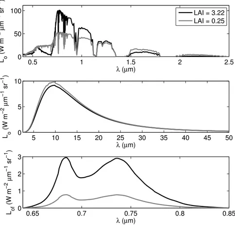
Figure 3 shows TOC radiance spectra in nadir direction, calculated using the input

spectra of Fig. 2 (linearly scaled such that total incoming shortwave (0.4–2.5µm)