First observations of global and seasonal terrestrial chlorophyll fluorescence from space

(1)

BGD

7, 8281–8318, 2010

Measurement of regional-scale

chlorophyll fluorescence

J. Joiner et al.

Title Page

Abstract Introduction

Conclusions References

Tables Figures

◭ ◮

Back Close

Full Screen / Esc

Printer-friendly Version Interactive Discussion

Discussion

P

a

per

|

Dis

cussion

P

a

per

|

Discussion

P

a

per

|

Discussio

n

P

a

per

|

Biogeosciences Discuss., 7, 8281–8318, 2010 www.biogeosciences-discuss.net/7/8281/2010/ doi:10.5194/bgd-7-8281-2010

Biogeosciences Discussions

This discussion paper is/has been under review for the journal Biogeosciences (BG). Please refer to the corresponding final paper in BG if available.

First observations of global and seasonal

terrestrial chlorophyll fluorescence from

space

J. Joiner1, Y. Yoshida2, A. P. Vasilkov2, Y. Yoshida3, L. A. Corp4, and E. M. Middleton1

1

NASA Goddard Space Flight Center, Greenbelt, MD, USA

2

Science Systems and Applications, Inc., 10210 Greenbelt, Rd., Ste 400, Lanham, MD, USA

3

National Institute for Environmental Studies (NIES), Tsukuba-City, Ibaraki, Japan

4

Sigma Space Corp., Lanham, MD USA

Received: 19 October 2010 – Accepted: 28 October 2010 – Published: 11 November 2010

Correspondence to: J. Joiner (joanna.joiner@nasa.gov)

(2)

BGD

7, 8281–8318, 2010

J. Joiner et al.

Title Page

Tables Figures

◭ ◮

Back Close

Full Screen / Esc

Discussion

P

a

per

|

Dis

cussion

P

a

per

|

Discussion

P

a

per

|

Discussio

n

P

a

per

|

Abstract

Remote sensing of terrestrial vegetation fluorescence from space is of interest because it can potentially provide global coverage of the functional status of vegetation. For ex-ample, fluorescence observations may provide a means to detect vegetation stress before chlorophyll reductions take place. Although there have been many

measure-5

ments of fluorescence from ground- and airborne-based instruments, there has been scant information available from satellites. In this work, we use high-spectral resolu-tion data from the Thermal And Near-infrared Sensor for carbon Observaresolu-tion – Fourier Transform Spectrometer (TANSO-FTS) on the Japanese Greenhouse gases Observ-ing SATellite (GOSAT) that is in a sun-synchronous orbit with an equator crossObserv-ing time

10

near 13:00 LT. We use filling-in of the potassium (K) I solar Fraunhofer line near 770 nm to derive chlorophyll fluorescence and related parameters such as the fluorescence quantum yield at that wavelength. We map these parameters globally for two months (July and December 2009) and show a full seasonal cycle for several diff_{erent locations,}

including two in the Amazonia region. We also compare the derived fluorescence

in-15

formation with that provided by the MODIS Enhanced Vegetation Index (EVI). These comparisons show that for several areas these two indices exhibit diff_{erent seasonality}

and/or relative intensity variations, and that changes in fluorescence frequently lead those seen in the EVI for those regions. The derived fluorescence therefore provides information that is related to, but independent of the reflectance.

20

1 Introduction

Vegetation is the functional interface between the Earth’s terrestrial biosphere and the atmosphere. Terrestrial ecosystems absorb approximately 120 Gt of carbon annually through the physiological process of photosynthesis. About 50% of the carbon is re-leased by ecosystem respiration processes within short time periods. The remaining

25

(3)

BGD

7, 8281–8318, 2010

J. Joiner et al.

Title Page

Tables Figures

◭ ◮

Back Close

Full Screen / Esc

Discussion

P

a

per

|

Dis

cussion

P

a

per

|

Discussion

P

a

per

|

Discussio

n

P

a

per

|

changes of ecosystems release parts of this carbon within the time frame of centuries. There are currently great uncertainties for the human impact on the magnitude of these processes.

Photosynthesis is the conversion by living organisms of light energy into chemical energy and fixation of atmospheric carbon dioxide into sugars; it is the key process

5

mediating 90% of carbon and water fluxes in the coupled biosphere-atmosphere sys-tem. Until now, most of the information that has been acquired by remote sensing of the Earth’s surface about vegetation conditions has come from reflected light in the solar domain. There is, however, one additional source of information about vegeta-tion productivity in the optical and near-infrared wavelength range that has not been

10

globally exploited by satellite observations. This source of information is related to the emission of fluorescence from the chlorophyll of assimilating leaves; part of the energy absorbed by chlorophyll cannot be used for carbon fixation and is thus re-emitted as fluorescence at longer wavelengths (lower energy) with respect to the absorption.

The fluorescence signal originates from the core complexes of the photosynthetic

15

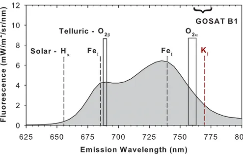
machinery where energy conversion of absorbed photosynthetically active radiation (APAR) occurs. Because the photosynthetic apparatus is an organized structure, the emission spectrum of fluorescence that originates from the photosynthetic apparatus is well known; it occurs as a convolution of broad band emission from 650 to 800 nm with two peaks in the visible and near-Infrared (NIR) at 685 and 740 nm, respectively,

20

as shown in Fig. 1 (e.g., Meroni et al., 2009; Corp et al., 2003, 2006).

The magnitude of the emission is variable and complex. Most studies have shown that in high light conditions (i.e., in the afternoon when many visible satellite measure-ments are made) and when plants are under stress, fluorescence is correlated with photosynthesis (van der Tol et al., 2009). Variations in fluorescence and

photosynthe-25

(4)

BGD

7, 8281–8318, 2010

J. Joiner et al.

Title Page

Tables Figures

◭ ◮

Back Close

Full Screen / Esc

Discussion

P

a

per

|

Dis

cussion

P

a

per

|

Discussion

P

a

per

|

Discussio

n

P

a

per

|

management, and assessment of the terrestrial carbon budget (e.g., Campbell et al., 2008).

To date, space-based approaches to provide insight into plant physiological sta-tus have relied primarily on the measured reflectance that provides information about chlorophyll content. There is observational evidence that chlorophyll fluorescence

sup-5

plies information content independent of reflectance-based spectral vegetation indices (e.g., Meroni and Colombo, 2006; Guanter et al., 2007; Meroni et al., 2008; Middleton et al., 2008, 2009). A measurement of chlorophyll fluorescence provides an important direct approach for diagnosing vegetation stress, associated with reduced photosyn-thetic functionality, before chlorophyll reduction occurs. It has therefore been a goal

10

of satellite missions proposed to the European Space Agency (ESA) and the United States National Aeronautics and Space Administration (NASA) (e.g., Davidson et al., 2003).

The measurement of solar-induced chlorophyll fluorescence,F, from space is chal-lenging, because its signal (typically 1–5% in the near-IR) must be diff_{erentiated from}

15

the much larger reflectance eff_ect. _F _{has been detected from ground- and}

airborne-based instrumentation by exploiting the fact thatF is a proportionally larger fraction of the total radiance within dark lines and bands of the atmospheric spectrum (e.g., Moya et al., 2004; Zarco-Tejada et al., 2009). These dark features include both very narrow solar Fraunhofer lines and wider telluric absorption features such as the O₂-B band at

20

687 nm and the O2-A band near 760 nm.

The O2 absorption features, primarily the O2-A band, have been used more exten-sively with recent ground-, aircraft-, and space-based spectrometers that have spectral resolutions of tenths of a nanometer and larger (individual lines not resolved), because these bands appear wider and deeper and align more closely with the peaks ofF (see

25

e.g., the review by Meroni et al., 2009, and more than 40 references within).

(5)

BGD

7, 8281–8318, 2010

J. Joiner et al.

Title Page

Tables Figures

◭ ◮

Back Close

Full Screen / Esc

Discussion

P

a

per

|

Dis

cussion

P

a

per

|

Discussion

P

a

per

|

Discussio

n

P

a

per

|

irradiance. In air- and space-borne applications, one must additionally account for absorption and scattering that takes place between the ground and instrument that further dilutes theF signal (e.g., Guanter et al., 2010).

Using an aircraft instrument with high spatial resolution, a measurement in a non-fluorescing pixel can be used to perform this atmospheric correction (e.g., Maier et al.,

5

2002, 2003). Rascher et al. (2009) mapped the relative distribution of fluorescence at 760 nm using a spectrometer mounted on an aircraft. They used an empirical normal-ization approach to correct for problems with radiometric calibration. In their approach, observations over bare soil at identical illumination conditions were used as a refer-ence.

10

The only space-based detection ofF to date was achieved by Guanter et al. (2007) with the MEdium Resolution Imaging Spectrometer (MERIS) (Rast et al., 1999) aboard the European Space Agency’s (ESA’s) ENVIronmental SATellite (ENVISAT). MERIS has two channels near the O₂-A band, one near the peak absorption at 760.6 nm with a 3.75 nm bandwidth, and one used as a reference band in the nearby continuum at

15

753.8 nm. MERIS makes measurements at a moderate spatial scale for land studies (better than 300 m per pixel in its Full Resolution mode).

The MERIS fluorescence retrieval was made for a limited area on one day. A radia-tive transfer model and other derived properties were used to correct for atmospheric eff_{ects and solve for the reflectance}_ρ _and _F_{. The derived} _F _{was compared with the}

20

other MERIS-derived biophysical products.

Here, instead of using O2-A band absorption, we make use of unique high spectral resolution measurements from the Japanese Greenhouse gases Observing SATellite (GOSAT). With GOSAT, we observe filling-in of the potassium (K) I solar Fraunhofer line near 770 nm. Though not designed for this purpose, we demonstrate that fluorescence

25

can be conclusively and directly measured from space and that GOSAT may be used to retrieveF at a regional scale.

(6)

BGD

7, 8281–8318, 2010

J. Joiner et al.

Title Page

Tables Figures

◭ ◮

Back Close

Full Screen / Esc

Discussion

P

a

per

|

Dis

cussion

P

a

per

|

Discussion

P

a

per

|

Discussio

n

P

a

per

|

dependence on surface albedo are shown in Sect. 3. Our approach for the retrieval of the chlorophyll fluorescence signal is given in Sects. 4–5. We show averaged monthly results for July and December 2009 in Sect. 6 along with full seasonal cycles for sev-eral regions. We also compare our fluorescence retrievals with the MODIS enhanced vegetation index (EVI). Conclusions are given in Sect. 7.

5

2 GOSAT observations

GOSAT is a satellite mission that was designed to monitor the global distribution of the greenhouse gases CO2and CH4(Yokota et al., 2009). It was jointly developed by the Japanese Ministry of the Environment (MOE), the National Institute for Environmental Studies (NIES), and the Japanese Aerospace Exploration Agency (JAXA). GOSAT was

10

launched on 23 January 2009 into a sun-synchronous orbit with a descending node equatorial crossing time near 13:00 LT. Its mean altitude is 666 km, and it has a 3 day repeat cycle.

Here we use spectra from the GOSAT Thermal And Near-infrared Sensor for car-bon Observation-Fourier Transform Spectrometer (TANSO-FTS) (Kuze et al., 2009).

15

The TANSO-FTS measures backscattered solar radiation in three shortwave infrared (SWIR) regions, referred to as “bands”, centered at 0.76, 1.6, and 2.0 µm. It has a nadir ground footprint of 10.5 km diameter.

GOSAT also has a Cloud and Aerosol Imager (CAI) with four bands at 0.38, 0.67, 0.87, and 1.6 µm with footprints between 0.5 and 1.5 km. The CAI was designed to

20

be used for detection and correction of cloud and aerosol eff_{ects in the TANSO-FTS}

spectra.

Chlorophyll fluorescence can be measured primarily within band 1 that extends from approximately 758 to 775 nm and encompasses the O2-A band. The primary function of the O2-A band for GOSAT is to account for the effects of cloud and aerosol within

25

(7)

BGD

7, 8281–8318, 2010

J. Joiner et al.

Title Page

Tables Figures

◭ ◮

Back Close

Full Screen / Esc

Discussion

P

a

per

|

Dis

cussion

P

a

per

|

Discussion

P

a

per

|

Discussio

n

P

a

per

|

0.356 cm−1(or approximately 0.022 nm), or a corresponding resolving power (ν/∆_ν_{) of}

>35000. Figure 2 shows the ILSF and spectral sampling within its FWHM. For a typical scene radiance (Lambertian surface albedo of 0.3 at 30◦_{solar zenith angle), the} signal-to-noise ratio (SNR) is>300.

3 Simulated effect of fluorescence on GOSAT measurements

5

Here, we simulate the eff_{ect of fluorescence on GOSAT observations in the vicinity of}

the K I line near 770 nm. We use the so-called KPNO2010 high spectral resolution solar irradiance reference spectrum (Chance and Kurucz, 2010), line parameters from the HITRAN 2004 database (Rothman et al., 2005), and a line-by-line code provided by R. Spurr (personal communication, 2010). Because Rayleigh optical thickness is low

10

at these wavelengths, we did not include atmospheric scattering in these simulations. Calculations were performed on a grid with spacing 0.01 cm−1

or 6e-4 nm. The solar spectrum was interpolated onto that grid.

Figure 3 shows simulated monochromatic and GOSAT reflectance spectra computed for a spectrally constant fluorescence of 3 mW/m2/sr/nm, solar zenith angle of 45◦_{, and}

15

a surface albedo of 0.2. The filling-in of the K I line near 770.1 nm is shown along with several O2 absorption lines including two weak lines on either side of the K I filling-in feature.

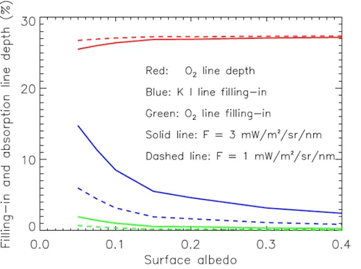
Figure 4 shows the dependence of the simulated filling-in of both the K I line and the 769.9 nm O2 line on the surface albedo for two values of fluorescence. The K I line

20

provides signficantly more filling-in than that of the O₂ line. The surface albedo has little eff_{ect on the O}₂ _{line depth, but does a}ff_{ect the observed filling-in, particularly of}

the K I line. The O2line depth depends on the satellite viewing geometry and surface pressure (not shown). The filling-in does not depend upon these parameters within the K I line, as there is no significant terrestrial absorption within this dark solar line.

(8)

BGD

7, 8281–8318, 2010

J. Joiner et al.

Title Page

Tables Figures

◭ ◮

Back Close

Full Screen / Esc

Discussion

P

a

per

|

Dis

cussion

P

a

per

|

Discussion

P

a

per

|

Discussio

n

P

a

per

|

4 Approach

Figure 5 shows both observed (normalized) solar irradiance and sample Earth-view radiance spectra from the TANSO-FTS band 1 and a zoom in at the wavelengths used here for fluorescence retrieval (bottom panel). Resolved lines within the O₂-A band are apparent in the Earth spectrum. Solar Fraunhofer lines are seen in both the

so-5

lar and Earth spectra. Note that there may be small errors in absolute wavelength calibration and that the asymmetric ILSF also produces an apparent wavelength shift between observations and exact positions of solar Fraunhofer lines. There may also be errors in the absolute radiometric calibration as the instrument radiometric sensitivity has decreased by about 10% from pre-flight values in band 1 and vicarious calibration

10

is required for correction.

The potassium (K) I line is one of the deepest solar Fraunhofer lines within GOSAT’s band 1 (∼755–775 nm). Although there are several other Fraunhofer lines lying closer

to the peak of the 740 nm fluorescence peak, the K I line was found to be the most ideal to observe chlorophyll fluorescence owing to its greater line depth and lack of

15

terrestrial oxygen absorption. The K I line falls between several weak O2lines and can be observed in relative isolation with GOSAT’s high spectral resolution.

The use of the K I line substantially simplifies a retrieval of F as compared with the O2-A band; atmospheric correction is not necessary as the absorption near it is negligible. The detection ofF using this method was thought to be unfeasible owing

20

to the high vegetation reflectance in the near-IR known as the red edge. However, at GOSAT’s high spectral resolution and SNR, and due to its large footprint that en-sures capture of substantial photon emissions, our simulations indicate that detection of ecosystem-scale chlorophyll fluorescence can be achieved.

We jointly retrieve the surface reflectivityρ (assumed Lambertian surface) and the

25

(9)

BGD

7, 8281–8318, 2010

J. Joiner et al.

Title Page

Tables Figures

◭ ◮

Back Close

Full Screen / Esc

Discussion

P

a

per

|

Dis

cussion

P

a

per

|

Discussion

P

a

per

|

Discussio

n

P

a

per

|

Earth spectral radianceI₍_λ_):

I₍_λ₎=_ρE₍_λ₎_/π+_F+∂I(λ)

∂∆_λ∆λ, (1)

whereE₍_λ_{) is the solar irradiance and} ∆_λ_{is the wavelength shift between Earth and}

solar spectra. Here, several GOSAT solar spectra taken closest in time to Earth radi-ance observations (within a few hours) are averaged together to produce a composite

5

spectrum. Before using Eq. (1), we first perform a rough adjustment to spectrally align the solar and Earth spectra. We then add the wavelength shift term in Eq. (1) to the fit to further improve the alignment.

Here, we assume a constant wavelength dependence of F and ρ over this band. This assumption could be relaxed as would be appropriate for a larger spectral fitting

10

window as discussed by e.g., Meroni et al. (2010). We could also account for scattering and absorption using a radiative transfer code. Note that the spectral dependence of atmospheric scattering is practically constant over this narrow window, so the neglect of it should have an insignificant eff_{ect on the retrieval of fluorescence. Similarly, a}

constant calibration off_{set in the solar irradiance will not a}ff_{ect the derived fluorescence}

15

as the error will be absorbed in the retrieved value ofρ. An error in absolute calibration ofI₍_λ_{), however, will be present in the retrieved}_F_.

The filling-in eff_{ect of rotational-Raman scattering at these wavelengths should be}

small as compared with theF signal (Sioris et al., 2003) at most observed solar zenith angles. Indeed, we found no evidence of a significant filling-in eff_{ect due to}

rotational-20

Raman scattering except at the highest solar zenith angles (SZA) when low PAR levels likely limit photosynthesis. These high SZA data were therefore eliminated from data shown here.

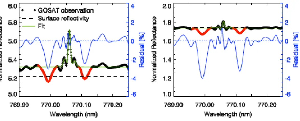
We use a standard weighted least squares fitting to derive ρ and F. There are two weak O2 lines located within the window, as shown by the red portions of the

25

reflectance spectra in Fig. 6. We eff_{ectively remove these wavelengths (769.96–770.02}

(10)

BGD

7, 8281–8318, 2010

J. Joiner et al.

Title Page

Tables Figures

◭ ◮

Back Close

Full Screen / Esc

Discussion

P

a

per

|

Dis

cussion

P

a

per

|

Discussion

P

a

per

|

Discussio

n

P

a

per

|

Our initial results showed positive values of fluorescence over the Sahara where none was expected. The root cause was found to be unexplained systematic spectral structure in the core of the K I line. An example is shown in the right panel of Fig. 6 for an observation taken over the Sahara. This spectral structure was initially fit by our algorithm as a small positive filling-in. We therefore found it necessary to adjust the

5

algorithm in order to account for this spectral structure. To accomplish this, we derived an average spectral signature of pixels where we expect zero fluorescence. Here we used clear-sky pixels from one day over the Sahara. We checked other days and obtained a similar result. We then added a term to account for this spectral structure, i.e.,

10

I₍_λ₎=ρE(λ)

π +F+ ∂I₍_λ₎

∂∆_λ∆λ+AH(λ), (2)

whereH₍_λ_{) is the derived mean radiance residual and}_A_{is the coe}ffi_{cient of the fit. This}

reduced the fluorescence bias over the Sahara and improved the fits to the radiance spectra globally.

We found that adding additional terms involving a polynomial in wavelength

expan-15

sion ofH₍_λ_{) provided a further improvement to the radiance fit and reduced the} stan-dard deviation of the radiance residuals, i.e.,

I₍_λ₎=ρE(λ)

π +F+ ∂I₍_λ₎

∂∆_λ∆λ+AH(λ)+BH(λ)(λ−λ0)+CH(λ)(λ−λ0)

2_, ₍₃₎

whereB and C are additional coeffi_{cients, and} _λ₀ _{is the wavelength in the center of}

our fitting window. With this treatment applied globally, the positive bias in

fluores-20

cence over the Sahara was eliminated, though a small negative bias in fluorescence remains there and elsewhere, particularly where fluorescence is near the detection limit. The largest adjustments toF using these terms are over the Sahara (on average

∼2–3 mW/m2/sr/nm) while adjustments elsewhere are smaller (∼1 mW/m2/sr/nm over inactive regions and 1.2–2 mW/m2/sr/nm over active vegetation). The majority of the

25

correction results from the use of theAcoeffi_{cient, but second order e}ff_{ects result from}

(11)

BGD

7, 8281–8318, 2010

J. Joiner et al.

Title Page

Tables Figures

◭ ◮

Back Close

Full Screen / Esc

Discussion

P

a

per

|

Dis

cussion

P

a

per

|

Discussion

P

a

per

|

Discussio

n

P

a

per

|

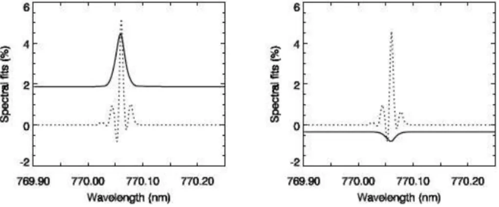
Examples of the fitted residual spectral structure are shown in Fig. 7 (dotted lines) for pixels over active vegetation in the Eastern United States (left) and Sahara (right). The fitted filling-in structure due to fluorescence (F/ρE₍_λ_{) in %) is also shown in Fig. 7.} Samples of the overall fits to normalized reflectance spectra for the same pixels are shown in Fig. 6 along with the fit residuals (observed minus fitted, %). For the

wave-5

lengths used in the fits, the residuals are generally within about±0.5%.

5 Further GOSAT data processing forF _retrievals

We first removed cloudy data by two diff_{erent methods. The remaining data were}

av-eraged in 2 degree latitude×2 degree longitude grid boxes. In the first cloud filtering

method, the concept of the cloud radiance fraction (CRF) is used. CRF is defined

10

as the fraction of pixel radiance coming from clouds. The CRF is a useful quantity for cloudy pixel screening because there can be situations of high cloud fractions with nearly transparent clouds that would minimally aff_{ect our retrievals, while there could}

also be cases of low cloud fractions but extremely bright clouds that we would not want to include in our sample. Here, we used CRF derived at 450 nm with the Ozone

Moni-15

toring Instrument (OMI) (Levelt et al., 2006) that flies on the Aura spacecraft. The CRF is supplied in the standard NO₂data product (Bucsela et al., 2006). OMI observations are made over the same geographical area within ∼<2 h of GOSAT. We used only

pixels with a cloud radiance fraction<10%.

In the second cloud filtering method, we used the cloud fraction from the GOSAT

20

CAI. Here, we removed pixels with estimated cloud fractions >10%. This provided results similar to those with the CRF. All results shown here use the second method.

We also examined radiance residuals in order to quality control the retrievals. We tested several diff_{erent thresholds on the residuals including a checks on the maximum}

residual and mean (over wavelength) residual. We found that some pixels exhibited

25

(12)

BGD

7, 8281–8318, 2010

J. Joiner et al.

Title Page

Tables Figures

◭ ◮

Back Close

Full Screen / Esc

Discussion

P

a

per

|

Dis

cussion

P

a

per

|

Discussion

P

a

per

|

Discussio

n

P

a

per

|

of samples per gridbox, leaving many gridboxes with no samples. Therefore, in the results shown below, we did not remove any pixels based on high radiance residuals.

The number of pixels averaged for a particular gridbox in a month varied from 1 to 39, with most grid boxes having between 2 and 12 observations. In dry areas with less clouds, like northern Africa, Saudi Arabia and central Australia, the number of

5

observations ranges from about 16–28 on average.

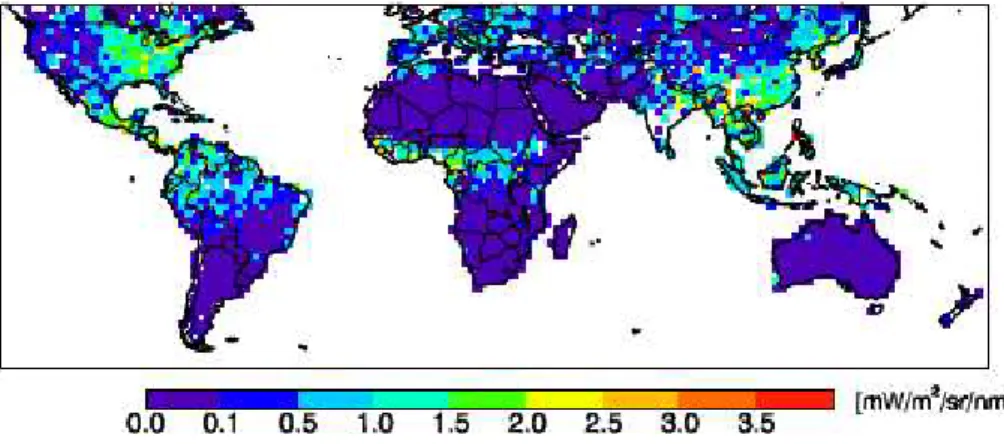
Figure 8 shows the retrieved monthly mean F for July 2009 in the same units as the Earth radiance. Another useful quantity that can be derived is the normalized instantaneous fluorescence quantum yield,Φ_{, given by}

Φ =_F_f_/_APAR=_F_f_/_(FPAR_×_PAR)_, ₍₄₎

10

(e.g., Louis et al., 2005), whereFf is the fluorescence flux, FPAR is the fraction of

ra-diation intercepted by the canopy, and PAR is the instantaneous (clear sky) broadband photosynthetically active radiation (400–700 nm). Here, we use FPAR derived from the MODerate-resolution Imaging Spectroradiometer (MODIS) (Myneni et al., 2002) as shown in Fig. 9. We estimated clean-sky PAR (no clouds or aerosol) using the radiative

15

transfer code of Fu and Liou (1992) and monthly mean total column ozone from OMI with ozone profile information from the GEOS-5 Data Assimilation System (Rienecker et al., 2007). We also used water vapor profiles from GEOS-5. Assuming that our de-rived fluorescence signal is isotropic, which is the traditional expectation, we may now estimateΦ _{for the narrow wavelength band (}_∼_{1 nm) considered here such that}Φ _is

20

unitless. Fig. 10 showsΦ_{(770 nm) for July 2009. As FPAR becomes small, any errors}

in theF, FPAR, or PAR become amplified. Therefore, we only showΦ_{for FPAR}_>₀_._3.

As the derivedΦ_{is somewhat noisy owing to the inclusion of incomplete information}

from other sensors, most subsequent results will be shown asF divided by cosine of the solar zenith angle (SZA), a proxy for PAR. We will refer to this as “scaled

fluores-25

(13)

BGD

7, 8281–8318, 2010

J. Joiner et al.

Title Page

Tables Figures

◭ ◮

Back Close

Full Screen / Esc

Discussion

P

a

per

|

Dis

cussion

P

a

per

|

Discussion

P

a

per

|

Discussio

n

P

a

per

|

we may consider scaledF, likeΦ_{, to be a unitless quantity. Note that this scaling}

am-plifies the retrieved small negative values of fluorescence that occur when we are near the detection limit; These negative values are prevalent at high solar zenith angles in the winter hemispheres when vegetation is inactive.

6 Results

5

Figure 11 shows monthly mean scaledF for July and December 2009 as retrieved from the K I solar line. The expected seasonal variation is definitively shown, namely, higher Northern Hemisphere terrestrial activity in July versus higher activity in the Southern Hemisphere in December. We also show the analogous data for the Enhanced Veg-etation Index (EVI) (Huete et al., 2002), a widely utilized vegVeg-etation reflectance-based

10

index to indicate relative greenness and to infer photosynthetic function, which was obtained over the same time periods from NASA’s Aqua MODIS sensor (Fig. 12). The Aqua satellite has an ascending node equator crossing near 13:30 LT, similar to that of GOSAT.

We compare and contrast the monthly averages for the derived and scaled F with

15

those for EVI, for the eight geographic regions outlined in Fig. 12. Although there are similarities between the scaledF and EVI values, some obvious diff_{erences are also}

evident. All of these plots show a large amount of scatter in the relationship between scaled F and EVI. Details of these diff_{erences are seen in the scatter diagrams of}

Figs. 13–15.

20

These continental or large regional blocks obviously include a variety of vegetation types such as forests, grasslands, and croplands that have diff_erent_F _{and EVI values.}

Even though the plots show significant scatter, for most regions there is an evident positive but non-linear relationship between F and EVI, but with a great deal of scatter. These trends are similar in shape and intensity value ranges in July in the Northern

25

(14)

BGD

7, 8281–8318, 2010

J. Joiner et al.

Title Page

Tables Figures

◭ ◮

Back Close

Full Screen / Esc

Discussion

P

a

per

|

Dis

cussion

P

a

per

|

Discussion

P

a

per

|

Discussio

n

P

a

per

|

Another example is that some regions display moderate EVI values (0.2–0.4) that imply the presence of green vegetation but where the fluorescence is at or near the detection threshold. This is particularly apparent in the July panel (Fig. 13, panel 5) for South America, which may indicate that the vegetation has retained greenness but is not physiologically active during the dry season.

5

Africa shows the most exciting example, with a clear positive and linear relationship for F:EVI across the observed greater range of F and EVI values in both July and December (Figs. 13 and 14.) This occurs because Africa spans both the northern and southern hemispheres and includes the full range of vegetation types, including the extremes of tropical forests and the Sahara desert. Indonesia, a tropical low latitude

10

region, shows no correlation between EVI and fluorescence and has the sameF:EVI cluster in both the July and December seasons.

Southern Hemisphere regions (Fig. 14) during the growing season (December) ex-hibit highly variableF versus EVI, with no clear relationships demonstrated here. South America and Australia show very low F in July (winter) over most of the EVI range

15

(<0.4).

Australia has mostly low to moderate EVI values during these months that show no correlation with fluorescence. The maps in Fig. 11 indicate that active fluorescence occurs over Australia primarily along the continental edges in the austral spring/early summer, a pattern not expressed distinctly in the corresponding EVI map.

20

Scatter diagrams using the scaled F are qualitatively similar to those using Φ

(Fig. 15), and have the advantage of reliance only on the GOSAT data. Moreover, the diagrams that use Φ _{show more variability and less correlation with EVI, most}

probably due to increased errors that result from inclusion of the MODIS FPAR satellite product. This further supports our use of the scaledF to demonstrate the capability of

25

the GOSAT sensor to measure chlorophyll fluorescence over land areas.

(15)

BGD

7, 8281–8318, 2010

J. Joiner et al.

Title Page

Tables Figures

◭ ◮

Back Close

Full Screen / Esc

Discussion

P

a

per

|

Dis

cussion

P

a

per

|

Discussion

P

a

per

|

Discussio

n

P

a

per

|

This seasonal cycle is also seen in the EVI which indicates a greater seasonal contrast (maximum vs. minimum) than the scaledF.

We next examine two Amazonia regions, one near the East coast of Brazil and one more towards the west in the central Amazon rainforest region (Fig. 16, panels 2–3). In the westernmost Amazon pixel (Fig. 16, panel 2), the dry season (July–November)

5

green up reported by Huete et al. (2006) for 2005 is seen here between September 2009 and January 2010 in both scaledF and EVI, with scaled F leading by approxi-mately one month beginning in August. In this region, trees with deep roots may have more continuous access to deep soil moisture (e.g., Nepstad et al., 1994). Here, EVI follows PAR which depends primarily on cloud cover and peaks during the dry season

10

(Huete et al., 2006). However, this temporal pattern is not captured in the MODIS Nor-malized Diff_{erence Vegetation Index (NDVI) (not shown); NDVI values typically peak in}

June/July for this region and decline to a minimum in December. In the other regions shown here, the NDVI is qualitatively similar (in the seasonal cycle) to the EVI.

In the eastern Amazon area (Fig. 16, panel 3), a diff_{erent pattern is seen with a}

15

brown-down in the early part of the dry season in both EVI and scaledF, consistent with analysis over grassland pasture sites in previous years by Huete et al. (2006). In this region, forest conversion has occurred where deep-rooted trees have been re-placed with shallow-rooted vegetation that responds more to soil moisture stress. The steepest decline in scaled F occurs from April to May, while a sharp decline in EVI

20

is seen from June through September. The scaled F shows an increase starting in September, while the EVI increase begins in October.

Over Indonesia (Fig. 16, panel 6), there is little seasonal change in EVI, although scaled F shows a significant minimum in June during the dry season when biomass burning typically takes place. El Ni ˜no began around this time in 2009 leading to a drier

25

(16)

BGD

7, 8281–8318, 2010

J. Joiner et al.

Title Page

Tables Figures

◭ ◮

Back Close

Full Screen / Esc

Discussion

P

a

per

|

Dis

cussion

P

a

per

|

Discussion

P

a

per

|

Discussio

n

P

a

per

|

In the north of Australia (Fig. 16, panel 7), EVI (and NDVI) generally peaks in the austral autumn owing to the summer monsoonal rains. In contrast, we see a more broad peak inF starting earlier. Higher spatial scale studies show significant variability in NDVI in this region as well as interannual variability (e.g. Martin et al., 2009). A dif-ferent pattern is seen in the EVI in the south western region of Australia with a distinct

5

peak in the spring (Fig. 16, panel 9). This pattern is not seen in the derived fluores-cence. These regions warrant further study and investigation into potential eff_{ects of}

sub-pixel variability and sources of error in the satellite-derived products.

7 Conclusions and ongoing work

While satellite-derived vegetation indices such as the EVI provide estimates of the

po-10

tential (or maximum) photosynthesis, the fluorescence retrievals shown here are the first regional-scale measures of actual (as compared with inferred potential) instanta-neous and dynamic photosynthetic activity derived by measuring light emission that originates from the cores of the photosynthetic machinery. Therefore, we do not nec-essarily expect to see a strong correlation between fluorescence and EVI. In fact, our

15

results indicate that our derived fluorescence is indeed providing information that is independent of EVI, and could be used to supplement it to provide important global productivity seasonal dynamics information. We intend to pursue this possibility fur-ther.

We have demonstrated that space-based missions that were specifically designed

20

to measure CO2 concentrations can also be used to measure an important value-added carbon product: regional-scale chlorophyll fluorescence. Further development of this product and studies using this data will help to maximize the benefits of space-based carbon missions such as GOSAT and a reflight of the NASA Orbiting Carbon Observatory (OCO) (Crisp et al., 2004).

(17)

BGD

7, 8281–8318, 2010

J. Joiner et al.

Title Page

Tables Figures

◭ ◮

Back Close

Full Screen / Esc

Discussion

P

a

per

|

Dis

cussion

P

a

per

|

Discussion

P

a

per

|

Discussio

n

P

a

per

|

The FLourescence EXplorer (FLEX) mission (Rascher, 2007; European Space Agency, 2008) was selected in 2006 for assessment as the result of the European Space Agency’s call for core Earth Explorer Mission ideas and has been since re-proposed. Our study provides evidence that such a mission could provide important information on photosynthetic effi_{ciency of terrestrial ecosystems at a global scale.}

5

This information combined with data from other satellites will help to better quantify relationships between the carbon and water cycles and their coupling with the Earth’s climate. The FLEX missions plans to utilize the O2-A band for chlorophyll fluorescence retrievals (Guanter et al., 2010), whereas OCO-2 could use the solar K Fraunhofer line since its spectral coverage and resolution is similar to GOSAT’s.

10

A chlorophyll fluorescence product may also be feasible from Geostationary (GEO) orbit using instrumentation being proposed for the NASA decadal survey GEO-Coastal and Air Pollution Events (GEO-CAPE) mission. This would provide important informa-tion regarding the links between pollutants, such as tropospheric O₃ that can damage vegetation, and climate, through the uptake of CO2, the primary anthropogenic

green-15

house gas.

As most previous studies ofF have been conducted at the leaf scale and at near-surface, care must be taken to properly interpret this large pixel data. The influence of canopy structure needs to be investigated in order to fully understand its influence on retrieved fluorescence and consequently derived relationships with key carbon-related

20

parameters such as gross primary production (GPP) and light-use effi_{ciency (LUE)}

(Damm et al., 2010).

We have reported fluorescence in appropriate units, and our values fall within the low end of ranges of other measurements reported in Meroni et al. (2009). We have not taken into account the directionality of the emitted fluorescence, although this is a

rea-25

(18)

BGD

7, 8281–8318, 2010

J. Joiner et al.

Title Page

Tables Figures

◭ ◮

Back Close

Full Screen / Esc

Discussion

P

a

per

|

Dis

cussion

P

a

per

|

Discussion

P

a

per

|

Discussio

n

P

a

per

|

large regions, will improve the understanding of this signal.

We are currently processing more GOSAT data in an eff_{ort to map global complete}

seasonal cycles and to quantify interannual variations in fluorescence owing to events such as extreme drought. We have also begun to examine our derived fluorescence in conjunction with satellite precipitation data.

5

Accounting for chlorophyll fluorescence in the K I line could assist in the interpreta-tions made forF in the O2-A band. Furthermore, this should also help to improve the retrieval of CO₂, as well as aerosol and cloud information from the O₂-A band. This band was designed to be an integral part of both the GOSAT and NASA OCO missions (e.g., Kuang et al., 2002; Crisp et al., 2004). It has been used with the SCanning

Imag-10

ing Absorption SpectroMeter for Atmospheric CHartographY (SCIAMACHY) to obtain an accurate description of the solar light path over both clear and cloudy pixels (Reuter et al., 2010) to aid in CO2retrievals. Without proper accounting for the variability of the fluorescence signal, the accuracy of CO₂, cloud, and aerosol information from these sensors will be degraded.

15

References

Bucsela, E. J., Celarier, E. A., Wenig, M. O., Gleason, J. F., Veefkind, J. P., Boersma, K. F., and Brinksma, E. J.: Algorithm for NO₂vertical column retrieval from the Ozone Monitoring Instrument, IEEE Trans. Geosci. Remote Sens., 44, 1245–1258, 2006. 8291

Campbell, E., Middleton, E. M., Corp, L. A., and Kim, M. S.: Contribution of chlorophyll

fluo-20

rescence to the apparent vegetation reflectance, Sci. Total Environ., 404, 433–439, 2008. 8284

Chance, K. and Kurucz, R. L.: An improved high-resolution solar reference spectrum for Earth’s atmosphere measurements in the ultraviolet, visible, and near infrared, J. Quant. Spec-trosc. Radiat. Trans., 111, 1289–1295, 2010. 8287

25

(19)

BGD

7, 8281–8318, 2010

J. Joiner et al.

Title Page

Tables Figures

◭ ◮

Back Close

Full Screen / Esc

Discussion

P

a

per

|

Dis

cussion

P

a

per

|

Discussion

P

a

per

|

Discussio

n

P

a

per

|

Corp, L. A., Middleton, E. M., McMurtrey, J. E., Campbell, P. K. E., and Butcher, L. M.: Fluo-rescence sensing techniques for vegetation assessment, Appl. Opt., 45, 1023–1033, 2006. 8283

Crisp, D.: The Orbiting Carbon Observatory (OCO) mission, Adv. in Space Res., 34, 700–709, 2004. 8296, 8298

5

Damm, A., Elbers, J., Erler, A., et al.: Remote sensing of sun-induced fluorescence to improve modeling of diurnal courses of gross primary production (GPP), Global Change Biology, 16, 171–186, doi:10.1111/j.1365-2486.200901908.x, 2010. 8297

Davidson, M., Berger, M., Moya, I., Moreno, J., Laurila, T., Stoll, M.-P., and Miller, J.: Mapping photosynthesis from space – a new vegetation-fluorescence technique, ESA Bull., 116, 34–

10

37, 2003. 8284

European Space Agency:. ESA SP-1313/4 Candidate Earth Explorer Core Missions - Reports for Assessment: FLEX – FLuorescence EXplorer, published by ESA Communication Produc-tion Office, Noordwijk, The Netherlands, http://esamultimedia.esa.int/docs/SP1313-4 FLEX. pdf., 2008. 8297

15

Fu, Q. and Liou, K.-N.: On the correlated k-distribution method for radiative transfer in nonho-mogeneous atmospheres, J. Atmos. Sci., 49, 2139–2156, 1992. 8292

Guanter, L., Alonso, L., G ómez-Chova, L., Amor ós-L ópez, J., Vila-Franc és, J., and Moreno, J.: Estimation of solar-induced vegetation fluorescence from space measurements, Geophys. Res. Lett., doi:10.1029/2007GL029289, 2007. 8284, 8285

20

Guanter, L., Alonso, L., G ´omez-Chova, Meroni, M., Preusker, R., Fischer, J., and Moreno, J.: Developments for vegetation fluorescence retrieval from spaceborne high-resolution spectrometry in the O₂-A and O₂-B absorption bands, J. Geophys. Res., 115, D19303, doi:10.1029/2009JD013716, 2010. 8285, 8297

Huete, A. R., Didan, K., Miura, T., Rodriguez, E. P., Gao, X., Ferreira, L. G.: Overview of the

25

radiometric and biophysical performance of the MODIS vegetation indices, Remote Sens, Environ,, 83, 195–213, 2002. 8293

Huete, A. R., Didan, K., Shimabukuro, Y. E., Ratana, P., and Saleska, S. R.: Ama-zon rainforests green-up with sunlight in dry season, Geophys. Res. Lett., 33, L06405, doi:10.1029/2005GL025583, 2006. 8295

30

(20)

BGD

7, 8281–8318, 2010

J. Joiner et al.

Title Page

Tables Figures

◭ ◮

Back Close

Full Screen / Esc

Discussion

P

a

per

|

Dis

cussion

P

a

per

|

Discussion

P

a

per

|

Discussio

n

P

a

per

|

Kuze, A., Suto, H., Nakajima, M., and Hamazaki, T.: Thermal and near infrared sensor for carbon observation Fourier-transform spectrometer on the Greenhouse Gases Observing Satellite for greenhouse gases monitoring, Appl. Opt., 48, 6716–6733, 2009. 8286

Levelt, P. F., van den Oord, G. H. J., Dobber, M. R., et al.: The Ozone Monitoring Instrument, IEEE Trans. Geosci. Rem. Sens., 44, 1093–1101, 2006. 8291

5

Louis, J., Ounis, A., Ducruet, J.-M., Evain, S., Laurila, T., Thum, T., Aurela, M., Wingsle, G., Alonso, L., Pedros, R., and Moya, I.: Remote sensing of sunlight-induced chlorophyll fluo-rescence and reflectance of Scots pine in the boreal forest during spring recovery, Remote Sens. Environ., 96, 37–48, 2005. 8292

Maier, S. W., G ¨unther, K. P., and Stellmes, M.: Remote sensing and modelling of solar induced

10

fluorescence, Proc. 1st Workshop Rem. Sens. Solar Induced Vegetation Fluorescence, ES-TEC, Noordwijk, The Netherlands, 19–20 June, 2002. 8285

Maier, S. W., G ¨unther, K. P., and Stellmes, M.: Sun-induced fluorescence: A new tool for precision farming, in: Digital imaging and spectral techniques: Applications to precision agri-culture and crop physiology, 209–222, edited by: VanToai, T., Major, D., McDonald, M.,

15

Schepers, J., and Tarpley, L., Madison, American Society of Agronomy, 2003. 8285

Martin, D., Grant, I., Jones, S., and Anderson, S.: Development of satellite vegetation indices to assess grassland curing across Australia and New Zealand, in: Innovations in Remote Sens-ing ad Photogrammetry, Lecture Notes in Geoinformation and Cartography, Part 3, edited by: Cartwright, W., Gartner, G., Meng, L., et al., Springer Berlin Heidelberg,

doi:10.1007/978-3-20

540-93962-7 17, 211–227, 2009. 8296

Meroni, M. and Colombo, R.: Leaf level detection of solar induced chlorophyll fluorescence by means of a subnanometer resolution spectroradiometer, Remote Sens. Environ., 103, 438–448, 2006. 8284

Meroni, M., Picchi, V., Rossini, M., Cogliati, S., Panigada, C., Nali, C., Lorenzini, G., Colombo,

25

R.: Leaf level early assessment of ozone injuries by passive fluorescence and photochemical reflectance index, Intl. J. Remote Sens., 29, 5409–5422, 2008. 8284

Meroni, M., Rossini, M., Guanter, L., Alonso, L., Rascher, U., Colombo, R., and Moreno, J.: Remote sensing of solar-induced chlorophyll fluorescence: Review of methods and applica-tions, Remote Sens. Environ., 113, 2037–2051, 2009. 8283, 8284, 8297

30

(21)

BGD

7, 8281–8318, 2010

J. Joiner et al.

Title Page

Tables Figures

◭ ◮

Back Close

Full Screen / Esc

Discussion

P

a

per

|

Dis

cussion

P

a

per

|

Discussion

P

a

per

|

Discussio

n

P

a

per

|

Middleton, E. M., Corp, L. A., and Campbell, P. K. E.: Comparison of measurements and FluorMOD simulations for solar induced chlorophyll fluorescence and reflectance of a corn crop under nitrogen treatments, Intl. J. Rem. Sensing, Special Issue for the Second Inter-national Symposium on Recent Advances in Quantitative Remote Sensing (RAQRSII), 29, 5,193–5,213, 2008. 8284

5

Middleton, E. M., Cheng, Y.-B., Corp, L. A., Huemmrich, K. F., Campbell, P. K. E. Zhang, Q.-Y., Kustas, W. P. and Russ, A. L.: Diurnal and seasonal dynamics of canopy-level solar-induced chlorophyll fluorescence and spectral reflectance indices in a cornfield, Proc. 6th EARSeL SIG Workshop on Imaging Spectroscopy, CD-Rom, 12 pp., Tel-Aviv, Israel March 16-19, 2009. 8284

10

Moya I., Camenen, L. Evain, S. et al.: A new instrument for passive remote sensing : 1. Mea-surements of sunlight-induced chlorophyll fluorescence. Remote Sens. Environ., 91, 186– 197, 2004. 8284

Myneni, R. B., Hoffman, W., Knyazikhin, Y., Privette, J. L., Glassy, J., Tian, Y., Wang, Y., Song, X., Zhang, Y., Smith, G. R., Lotsch, A., Friedl, M., Morisette, J. T., Votava, P., Nemani, R. R.,

15

and Running, S. W.: Global products of vegetation leaf area and fraction absorbed PAR from year one of MODIS data. Remote Sens. Environ., 83, 214–231, 2002. 8292

Nepstad, D. D., de Carvalho, C. R., Davidson, E. A., Jipp, P. H., Lefebvre, P. A., Negreiros, G. H., da Silva, E. D., Stone, T. A., Trumbore, S. E., and Vieira, S.: The role of deep roots in the hydrological and carbon cycles of Amazonian forests and pastures. Nature, 372, 666–669,

20

1994. 8295

Rascher, U.: FLEX – Fluorescence Explorer: A remote sensing approach to quatify spatio-temporal variations of photosynthetic efficiency from space, Photosynth. Res., 91, 293–294, 2007. 8297

Rascher, U., I. Agati, L. Alonso, et al.: CEFLES2: the remote sensing component to quantify

25

photosynthetic effi_{ciency from the leaf to the region by measuring sun-induced fluorescence}

in the oxygen absorption bands. Biogeosci., 6, 1181–1198, 2009. 8285

Rast, M. J., B ´ezy, J. L., and Bruzzi, S.: The ESA Medium Resolution Imaging Spectrometer MERIS - A review of the instrument and its mission. Int. J. Remote Sens., 20, 1681–1702, 1999. 8285

30

(22)

BGD

7, 8281–8318, 2010

J. Joiner et al.

Title Page

Tables Figures

◭ ◮

Back Close

Full Screen / Esc

Discussion

P

a

per

|

Dis

cussion

P

a

per

|

Discussion

P

a

per

|

Discussio

n

P

a

per

|

Rienecker, M. M., Suarez, M. J., Todling, R., et al.: The GEOS5 data assimilation system -Documentation of versions 5.0.1, 5.1.0, and 5.2.0. NASA Tech. Memo. 2007-104606, vol. 27, M. J. Suarez, Editor., 2007. 8292

Rothman, L. S., Jacquemart, D., Barbe, A., et al.: The HITRAN 2004 molecular spectroscopic database, J. Quant. Spectrosc. Radiat. Trans., 96, 139–204, 2005. 8287

5

Sioris, C., Courr `eges-Lacoste, G. B. and Stoll M. P.: Filling in of Fraunhofer lines by plant fluorescence: Simulations for a nadir-viewing satellite-borne instrument. Geophys. Res. Lett., 108, 4133, doi:10.1029/2001JD001321, 2003. 8289

van der Tol, C., Verhoef, W., and Rosema, A.: A model for chlorophyll fluorescence and photo-synthesis at leaf scale, Agricult. Forest Meteorol., 149, 96–105, 2009. 8283

10

Yokota, T., Yoshida, Y., Eguchi, N., Ota, Y., Tanaka, T., Watanabe, H., and Maksyutov, S.: Global Concentrations of CO₂ and CH₄ Retrieved from GOSAT: First Preliminary Results, Sci. Online Lett. Atm., 5, 160–163, 2009. 8286

Zarco-Tejada, P. J., Berni, J. A. J., Suarez, L., Sepulcre-Cant ´o, G., Morales, F., and Miller, J. R.: Imaging chlorophyll fluorescence with an airborne narrow-band multispectral camera

15

(23)

BGD

7, 8281–8318, 2010

J. Joiner et al.

Title Page

Tables Figures

◭ ◮

Back Close

Full Screen / Esc

Discussion

P

a

per

|

Dis

cussion

P

a

per

|

Discussion

P

a

per

|

Discussio

n

P

a

per

|

Fig. 1. Simulated solar-induced fluorescence as a function of the emission wavelength with

(24)

BGD

7, 8281–8318, 2010

J. Joiner et al.

Title Page

Tables Figures

◭ ◮

Back Close

Full Screen / Esc

Discussion

P

a

per

|

Dis

cussion

P

a

per

|

Discussion

P

a

per

|

Discussio

n

P

a

per

|

Fig. 2.GOSAT instrument line shape function with spectral sampling indicated in the full-width

(25)

BGD

7, 8281–8318, 2010

J. Joiner et al.

Title Page

Tables Figures

◭ ◮

Back Close

Full Screen / Esc

Discussion

P

a

per

|

Dis

cussion

P

a

per

|

Discussion

P

a

per

|

Discussio

n

P

a

per

|

Fig. 3.Simulated monochromatic and GOSAT reflectance spectra assuming a fluorescence of

(26)

BGD

7, 8281–8318, 2010

J. Joiner et al.

Title Page

Tables Figures

◭ ◮

Back Close

Full Screen / Esc

Discussion

P

a

per

|

Dis

cussion

P

a

per

|

Discussion

P

a

per

|

Discussio

n

P

a

per

|

Fig. 4. Simulated GOSAT filling-in of and absorption from the O₂weak line at 769.9 nm and

(27)

BGD

7, 8281–8318, 2010

J. Joiner et al.

Title Page

Tables Figures

◭ ◮

Back Close

Full Screen / Esc

Discussion

P

a

per

|

Dis

cussion

P

a

per

|

Discussion

P

a

per

|

Discussio

n

P

a

per

|

Fig. 5. GOSAT solar and Earth spectra in band 1 with the K I line (top) and zoom near the

(28)

BGD

7, 8281–8318, 2010

J. Joiner et al.

Title Page

Tables Figures

◭ ◮

Back Close

Full Screen / Esc

Discussion

P

a

per

|

Dis

cussion

P

a

per

|

Discussion

P

a

per

|

Discussio

n

P

a

per

|

Fig. 6. Normalized reflectance (Earth radiance normalized by the solar spectra, black and red

(29)

BGD

7, 8281–8318, 2010

J. Joiner et al.

Title Page

Tables Figures

◭ ◮

Back Close

Full Screen / Esc

Discussion

P

a

per

|

Dis

cussion

P

a

per

|

Discussion

P

a

per

|

Discussio

n

P

a

per

|

Fig. 7. Fitted unexplained (dotted) and fluorescence (solid) spectral structure as a percent of

(30)

BGD

7, 8281–8318, 2010

J. Joiner et al.

Title Page

Tables Figures

◭ ◮

Back Close

Full Screen / Esc

Discussion

P

a

per

|

Dis

cussion

P

a

per

|

Discussion

P

a

per

|

Discussio

n

P

a

per

|

Fig. 8. Derived monthly averages for instantaneous fluorescence F (mW/m2/sr/nm) from

(31)

BGD

7, 8281–8318, 2010

J. Joiner et al.

Title Page

Tables Figures

◭ ◮

Back Close

Full Screen / Esc

Discussion

P

a

per

|

Dis

cussion

P

a

per

|

Discussion

P

a

per

|

Discussio

n

P

a

per

|

(32)

BGD

7, 8281–8318, 2010

J. Joiner et al.

Title Page

Tables Figures

◭ ◮

Back Close

Full Screen / Esc

Discussion

P

a

per

|

Dis

cussion

P

a

per

|

Discussion

P

a

per

|

Discussio

n

P

a

per

|

Fig. 10.Derived monthly averages for instantaneous fluorescence quantum yield,Φ, (unitless)

(33)

BGD

7, 8281–8318, 2010

J. Joiner et al.

Title Page

Tables Figures

◭ ◮

Back Close

Full Screen / Esc

Discussion

P

a

per

|

Dis

cussion

P

a

per

|

Discussion

P

a

per

|

Discussio

n

P

a

per

|

Fig. 11.Derived monthly averages for scaled fluorescence (unitless) from GOSAT for July and

(34)

BGD

7, 8281–8318, 2010

J. Joiner et al.

Title Page

Tables Figures

◭ ◮

Back Close

Full Screen / Esc

Discussion

P

a

per

|

Dis

cussion

P

a

per

|

Discussion

P

a

per

|

Discussio

n

P

a

per

|

Fig. 12.Enhanced Vegetation Index (EVI) (unitless) from Aqua MODIS for July and December

(35)

BGD

7, 8281–8318, 2010

J. Joiner et al.

Title Page

Tables Figures

◭ ◮

Back Close

Full Screen / Esc

Discussion

P

a

per

|

Dis

cussion

P

a

per

|

Discussion

P

a

per

|

Discussio

n

P

a

per

|

Fig. 13.Scatter plots of the GOSAT scaled fluorescence versus the MODIS enhanced

vegeta-tion index (EVI) (both unitless) for July 2009 for different regions shown in Fig. 12. Each point represents a monthly mean from a single 2◦

(36)

BGD

7, 8281–8318, 2010

J. Joiner et al.

Title Page

Tables Figures

◭ ◮

Back Close

Full Screen / Esc

Discussion

P

a

per

|

Dis

cussion

P

a

per

|

Discussion

P

a

per

|

Discussio

n

P

a

per

|

Fig. 14. Similar to Fig. 13 but showing scaled fluorescence versus the MODIS enhanced

(37)

BGD

7, 8281–8318, 2010

J. Joiner et al.

Title Page

Tables Figures

◭ ◮

Back Close

Full Screen / Esc

Discussion

P

a

per

|

Dis

cussion

P

a

per

|

Discussion

P

a

per

|

Discussio

n

P

a

per

|

Fig. 15.Similar to Fig. 13 but showing derived fluorescence quantum yield,Φ, versus MODIS

(38)

BGD

7, 8281–8318, 2010

J. Joiner et al.

Title Page

Tables Figures

◭ ◮

Back Close

Full Screen / Esc

Discussion

P

a

per

|

Dis

cussion

P

a

per

|

Discussion

P

a

per

|

Discussio

n

P

a

per

|

Fig. 16. Bottom panel: Full seasonal cycle in scaled F (left axis, unitless) for the regions