Systematical detection of significant genes in microarray data by incorporating gene interaction relationship in biological systems.

(1)

Microarray Data by Incorporating Gene Interaction

Relationship in Biological Systems

Junwei Wang1, Meiwen Jia1, Liping Zhu2, Zengjin Yuan1, Peng Li1, Chang Chang1, Jian Luo1, Mingyao Liu1, Tieliu Shi1*

1The Center for Bioinformatics and Computational Biology, The Institute of Biomedical Sciences, The School of Life Sciences, East China Normal University, Shanghai, China,2The College of Financial and Statistics, East China Normal University, Shanghai, China

Abstract

Many methods, including parametric, nonparametric, and Bayesian methods, have been used for detecting differentially expressed genes based on the assumption that biological systems are linear, which ignores the nonlinear characteristics of most biological systems. More importantly, those methods do not simultaneously consider means, variances, and high moments, resulting in relatively high false positive rate. To overcome the limitations, the SWangtest is proposed to determine differentially expressed genes according to the equality of distributions between case and control. Our method not only latently incorporates functional relationships among genes to consider nonlinear biological system but also considers the mean, variance, skewness, and kurtosis of expression profiles simultaneously. To illustrate biological significance of high moments, we construct a nonlinear gene interaction model, demonstrating that skewness and kurtosis could contain useful information of function association among genes in microarrays. Simulations and real microarray results show that false positive rate ofSWangis lower than currently popular methods (T-test, F-test, SAM, and Fold-change) with much higher statistical power. Additionally,SWangcan uniquely detect significant genes in real microarray data with imperceptible differential expression but higher variety in kurtosis and skewness. Those identified genes were confirmed with previous published literature or RT-PCR experiments performed in our lab.

Citation:Wang J, Jia M, Zhu L, Yuan Z, Li P, et al. (2010) Systematical Detection of Significant Genes in Microarray Data by Incorporating Gene Interaction Relationship in Biological Systems. PLoS ONE 5(10): e13721. doi:10.1371/journal.pone.0013721

Editor:Mary Bryk, Texas A&M University, United States of America

ReceivedMarch 18, 2010;AcceptedOctober 5, 2010;PublishedOctober 29, 2010

Copyright:ß2010 Wang et al. This is an open-access article distributed under the terms of the Creative Commons Attribution License, which permits unrestricted use, distribution, and reproduction in any medium, provided the original author and source are credited.

Funding:This work was supported by the State Key Program of Basic Research of China grants (2010CB945400, 2007CB108800, 2009CB918400), the National High Technology Research and Development Program of China (863 project) (Grant No. 2006AA02Z313) and National Natural Science Foundation of China grants (30870575). The funders had no role in study design, data collection and analysis, decision to publish, or preparation of the manuscript.

Competing Interests:The authors have declared that no competing interests exist.

* E-mail: tlshi@sibs.ac.cn

Introduction

DNA microarray technologies have been widely used in biological studies, and simultaneously measure expression levels of thousands of genes across cells or tissues under different conditions [1]. In the microarray data analysis process, one of the most important steps is to determine whether a gene is differentially expressed under particular conditions since follow-up analysis depends on the selected differentially expressed genes (DEGs). Nevertheless, the selection of the DEGs is associated with both statistical and biological problems [2]. The biological problem is whether the identification of DEGs should consider nonlinear biological system. Practically, gene interactions are nonlinear [3–5]. In nonlinear systems such parameters (mean, variance, skewness, kurtosis) can be interdependence [6], where skewness and kurtosis are defined as nonlinear index [7] and can be preserved even in a weakly nonlinear network or system [8,9]. When an input signal follows normal distribution, nonlinear system (e.g., quadratic) can produce an output signal with non-Gaussian distribution [7,9]. Hence, skewness and kurtosis should be used in evaluating nonlinear systems. Statistically, some current existing tests for DEGs detection assume linear relationships, Normal distribution, and large sample sizes according to the

classical statistics. In fact, the limitation of resources and high cost of the microarray experiments make the sample sizes usually much smaller relative to the number of considered genes, which results in the decrease of the statistical power (SP), high false positive rate (FPR), and the enlargement of sample’s error [10].

(2)

In contrast, other methods, such as Hartley, Cochran, and Bartlett test, could utilize sample variance difference to detect DEGs. These methods identify DEGs without considering the difference between means based on an assumption that the logarithm of expression-level measurement of a gene under a given condition has a rough Gaussian distribution. Meanwhile, non-parametric methods without any distribution hypothesis have also been used to select differentially expressed genes, but much information is ignored because those methods only considerate the rank of samples.

Alternatively, other methods have been developed to detect DEGs on the basis of large-scale data, or statistical models. The false discovery rate (FDR) [16], ranking analysis of microarray data (RAM) [17], FDR-base methods [17], and optional discovery procedure (ODP) [18] identify DEGs through ranking the statistics of any statistical method based on large-scale data. FDR, an expected proportion of the false positive among all the positives detected, is to control the erroneous rejection of a number of true null hypotheses, while RAM is a large-scale two-sample t-test method and is based on the comparisons among a set of ranked T statistics. Hence, the first step of FDR and RAM is to calculate statistics of each gene in a microarray. In the application of ODP, the assumption of the null distribution and alternative distribution is the prerequisite. Hotelling’ T2test is to test the different mean vectors of entirety genes of case-control, yet it is still limited by the smaller sample sizes relative to the number of considered genes. The MFS-Hotelling’ T2[19] is not affected by sample sizes but is still based on means and covariance. Those methods are designed for large-scale data, while other methods based on statistical models have been proposed, like Bayesian method included probe-level measurement error (BPLME) [14], and FS test [20]. BPLME employs Bayesian hierarchical models to estimate probe-level measurement error which is utilized to adjust the variance for selecting DEGs. Similar to ANOVA and F-test, FStest is based on generalized linear model to estimate shrinking variance to determine DEGs. Although these methods may be robust in finding DEGs to a certain extent, they all ignore the information of the high moments.

Unlike other methods, ANOVA, a generalization of thet-test, allows for the comparison for more than two conditions’ samples. Similarly, F-test, fixed-ANOVA, and mixed-ANOVA are designed to detect DEGs under several conditions [21]. However, they only consider the information of the locations.

In all, current published methods are adjusted basic statistics methods and try to decrease the FPR in microarray analysis according to aforementioned approaches. Those methods only focus on difference of location or variance and ignore the difference of high moments, which could possibly lead to error in certain parts of randomization theory [22]. Moreover, they also ignore the functional association from those functionally related genes in microarray experiments because they assume that biological systems are linear and their approaches follow Normal distribution, respectively. During the process of DEGs selection, those statistical methods simply discard the genes which may actually be quite important because they display insignificance in different means or variances between case and control. Therefore, those methods normally have comparatively low statistics power with high FPR [10]. It is still a challenge that how to improve SP and maximally extract the useful information from the microarray data by incorporating the information about the functional relationship between genes from the microarray data with relatively small sample size [10].

To decrease FPR and improve SP, we present theSWangtest to detect the DEGs not only by utilizing means, variances, skewness, and kurtosis simultaneously, but also by recognizing and latently

incorporating the functional relationship of genes in biological systems. In the study, we conduct comparative evaluation of the performance betweenSWang and other tests, like T-test, F-test, SAM, and Fold-change, based on simulated and real microarray data. Two real microarray datasets of breast cancer are employed to testSWangmethod and other four tests. Moreover, we carry out experiments at the bench to confirm those genes uniquely identified as being differentially expressed bySWang(1,4). All the results demonstrate that our method is superior to the other four statistics methods for the DEGs detection.

SWangtest has several unique characteristics compared to the current popular methods.

First, SWang utilizes the information of multiple and high moments which have been used to summarize the shape of a probability distribution in probability theory (File S1 text). The high moments represent certain information of distributions, e.g., the skewness indicating symmetric distribution. The positive skewness means the asymmetric distribution with longer right tail while negative skewness indicates the asymmetric distribution with longer left tail [23]. Therefore, the first moment (also known as mean) could not be enough to represent all the location information in asymmetric distribution. The positive kurtosis means that most of the variance is the result of infrequent extreme deviations, as opposed to frequent modestly sized deviations [23]. To illustrate the biological significance of high moments, we construct a nonlinear gene interaction model to demonstrate that high moments contain the information of association among genes. Although the estimated high moments may be biased, the estimation of kurtosis could be reliable in Pearson’ distribution family with relatively small sample size [23] and they are necessary to be considered in detecting DEGs. Because the sample size is much smaller than the size of genes under most circumstances in the microarray application, and the small sample size makes the law of large number invalid [24,25], it indicates that the mean and variance contain insufficient information of the data when the sample size is small.

Second, we assume that the distribution of gene expression profile belongs to Pearson distribution family that includes normal distribution, exponential distribution, Gammas distribution, or mixture of Gaussian/Gammas distribution, according to previous studies [25–27].

Third, from the statistical view, the highest moment for the samples should be four and the fourth moment corresponds to kurtosis [22]. Our method realizes and utilizes multiple moments simultaneously, since it can also be statistically proven that the high moment is necessary and essential for the gene differential expression detection under the small sample size.

Fourth, SWang latently incorporates the biological facts that functionally related genes have effects on the expression levels of one another. Although the associations among genes are not easy to be estimated, they could be recognized via considering all moments according to nonlinear gene interaction model and nonlinear biological system.

Finally, SWang can be used to detect DEGs with different combinations of different moments which depend on the sample size and the assumption of distribution.SWangis based on a null hypothesis that the mean, variance, skewness, and kurtosis between case and control should be equal. Although there are total of 15 combinations, we suggest that it is better to consider the four different moments simultaneously during the application.

Results

(3)

under Pearson distribution family betweenSWangand four other methods, including T-test, F-test, SAM(s0 = 0.3), Fold-change. The first simulation was to calculate FPR without considering gene associations under various distributions and the second was to measure SP with the consideration of nonlinear biological system. Next, DEGs were selected in real microarray data with those methods. During the processes, the criteria for p-value and q-value are 0.05 (or 2-fold change), and these rigorous criteria are to minimize the false positive results [28]. Subsequently, the results generated with those five different methods are compared with each other. Additionally, we also use ‘spike-in’ data to evaluate the SWang.

Firstly, we randomly drew samples from both case and control groups. The distribution of case group was considered as exponential, normal, uniform, cauchy distribution, complex of triangular, normal, and exponential distribution, or mixture of normal distribution, respectively, when the distribution of control group was regarded as normal distribution with mean as 1 and standard deviation as 1.5. Sample size was the combination of the sample size of both case and control from 3 to 53 (Details inFile S4). This step is to generate a pair of case and control groups for a gene of interest to test whether the gene is differentially expressed. During simulation, we randomly assigned 20% genes as DEGs to calculate false positive rate when the distributions of case and control are the same and explore the differences of skewness and kurtosis between case and control from either small samples or real gene-expression variation. Then we calculated the p-value of SWang, T-test, SAM, and F-test or fold-change ratio. Subsequent-ly, we counted the number of those genes withp-value less than 0.05 or fold change greater than 2. Finally, we calculated the FPR and SP of each method [29].

Next, we drew the figures with false positive rate as vertical coordinate and cut-off p-value as horizontal coordinate according to the simulation results. The cut-off p-value is the theoretical false positive rate which is the ratio of undifferentially expressed genes selected as DEGs to the total number of DEGs in theory. The false positive rate is the real p-value generated from the simulation results. Practically, if the curve in generated figures is above diagonal line, it indicates that the real false finding ratio is higher than estimated false finding ratio, and the method is unconvincing, so that the result obtained by this method is undesirable with low confidence. In contrast, if the curve is on or below the diagonal line, the real false finding ratio is equal to or less than the estimated false finding ratio, resulting in the satisfied findings with high confidence.

The results showed that the curves of F-test, T-test, andSWang displayed lower false positive rate with their curves on or below the diagonal line, with the curve of SWang located at lowest level (Figure 1).

Traditionally, the microarray data are regarded to follow normal distribution. We tested the performance of SWang and others under this assumption. Comparing the curves generated from other methods, the slope value of the curve forSWangwith different combinations of moments and different sample sizes are the smallest. It can be seen that the separation ability for the curve between SWang and others is largest when fourth moment (kurtosis) is applied inSWangto detect DEGs. Simulation results also show that the FPRs of SWang with high moments are the lowest among all the tested methods, regardless of the sample size (Figure S4).

In fact, the real microarray data distribution does not always fit normal distribution. Therefore, we considered the situation that the distribution of microarray data belongs to Pearson distribution family, and also tested the performance of SWang and other

methods under various Pearson distributions. Exponential distri-bution is a special gamma distridistri-bution which is a subset of Pearson distribution family. The curves generated from those methods indicate that the slope of the curve forSWangis the most gradual. The FPR ofSWangwith high moments are the lowest with sample size greater than 5 (Figure S6). We obtained the similar results on other Pearson distribution including Uniform distribution, and Cauchy distribution.

The results fromFigure 1, andFigure S1,S2,S3,S4,S5,S6, S7demonstrated that our methods have good performance with higher confidence in DEGs detection, and that the differences of skewness and kurtosis between case and control are not due to the sample size but to real gene-expression variation. When high moments are utilized, FPRs ofSWangare less than those of other methods. As the sample size increases, the significance of skewness and kurtosis correspondingly decreases.

We also verified the effectiveness ofSWang with the ‘spike-in’ data [30] that contain a limited number of spiked-in cRNAs. The ‘spike-in’ data is a control dataset which has been used for evaluating the effectiveness of analysis methods for microarrays. This dataset has several features to facilitate the relative assessment of different analysis options [30]. Our analysis demonstrated that the SWang(1,4) option provided the lowest false positive rate (Figure S8). The other options of SWang proved less effective compared to the SAM and Fold-change methods, this could be due to the criteria in ‘spike-in’ experimental design for selecting DEGs solely based on Fold-change. In addition, the experimental design for the ‘spike-in’ data may not even have considered gene function associations.

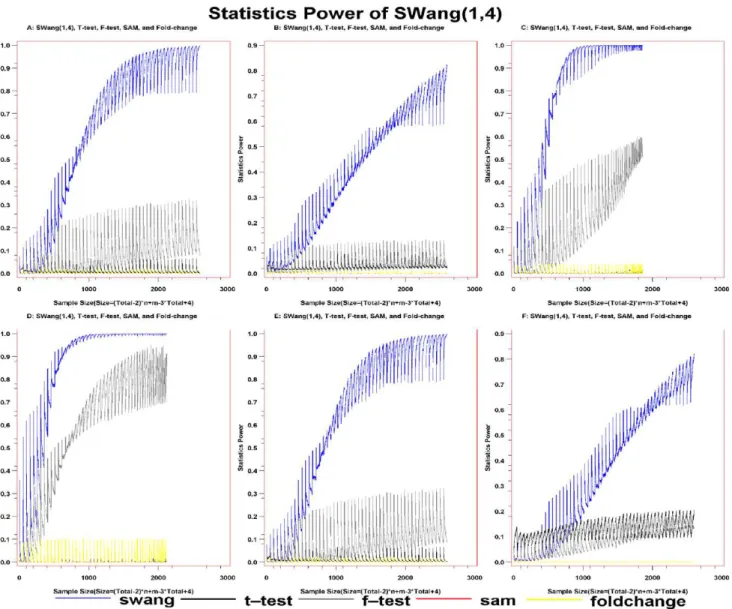
We then evaluated the robustness of SWang with simulation when considering nonlinear biology system (Figure 2, and Figure S8, S9, S10, S11, S12, S13, S14, S15). The sample size is the combination of the sample sizes from both case and control groups and the SP is the ratio of the number of DEGs to the total genes generated from the simulation results. Visually, the far the curve in the figures from the horizontal coordinate, the better the method.

Under normal distribution, the curve of theSWang(1,4) option is on the top, the curve of F-test is the second, below that of SWang(1,4), and the curves of the other three methods separate from that ofSWangand F-test significantly, being close to baseline (Figure 2A). More interestingly, under Exponential distribution, the curve ofSWang(1,4) is on the top and far apart from the curves of other four methods (Figure 2B). Similar results can be observed under Uniform, Gamma, mixture of Gamma and Normal, and complex distribution (Figure 2C–2F). When the sample size is very small, it seems that the curves ofSWangand the other four methods cannot be distinguished. To further compare SP betweenSWangand the other four methods under small sample size, we drewFigure S9 with small sample size and the result illustrates that the curves using theSWang(1,4) option are still on the top. Therefore, it is shown that SP ofSWangis always larger than other methods under various tested distributions, indicating thatSWanghas the best performance among those five methods.

(4)

S11). Simulation results under other Pearson distribution family also showed that the curves ofSWang(1,3) andSWang(1,4) to be far above the curve of other methods (Figure S12, S13,S14,S15, S16). These analyses demonstrate that SPs of SWang(1,3) and SWang(1,4) are larger than those of the other methods, and that it is necessary to utilize high moments to detect DEGs.

To evaluate the performance of our method on real data, we used theSWang(1,4) option to detect the DEGs in both dataset1 and dataset2 related to breast cancer (See Material & Method), and then mapped those selected genes to human biological pathways based on the KEGG system. Here, we only focus on those genes that are mapped to the cancer related pathways from KEGG.

In Dataset1, the previous study has identified 160 significantly differentially expressed genes at threshold ofqvalues#0.05 [28]. In the same dataset, our method detected 157 genes with differential expression in those 160 genes. The three genes that are not selected

by our method all have higherp-value in our result, although theq -value for those genes is less than 0.05 based on previous method. Thep-value for gene CKS2 (Mutation Id 359119) with our method is 0.05667 when itsq-value is 0.04540; gene MYCLK1 (Mutation Id 417226) has a q-value of 0.04723, but its p-value based on our method is 0.05011; meanwhile, the Mutation Id (HV18H8) corresponding to an unknown gene is also detected as differentially expressed with aq-value of 0.04984 based on previous study, but in our result itsp-value is 0.055762, larger than 0.05.

(5)

additionally detected 42 genes (63 Mutation Id) in Dataset1, 312 genes (362 probes) in Dataset2 as differentially expressed. Although there are larger number of genes detected by F-test and T-test than that of genes selected bySWang, T-test and F-test have higher FPR with respect to non-Gaussian distribution of microarray [19]. Moreover, T-test and F-test ignore the nonlinear biology system. The inherent limitations of the two tests could bring about high positive result.

To further confirm the results of our analysis, we randomly selected 9 genes from those genes detected by T-test, F-test, SAM(0.3), or Fold-change but not detected by our method in Dataset2, and carried out the same RT-PCR experiment. Because some of the gene names do not exist in NCBI anymore and the RT-PCR for some other genes was unsuccessful, eventually, we got RT-PCR result for 3 out of 9 genes. The result shows that those three genes are not differentially expressed between the breast cancer lines and control (Figure S20).

In dataset1, we focused on those uniquely selected genes (Table S1 in File S5) that are involved in the related cancer pathways. The relative statistics for those genes are listed in Table 1. TP53 (GeneID: 7157) was one of gene selected which encodes a tumor suppressor, that has been widely recognized as an important protein in various carcinogenesis. It is one of the components in MAPK signaling pathway [31]. Changes in the TP53 gene greatly increase the risk of developing breast cancer [32], [33–35]. TP53-mutated breast cancers have been shown increased sensitivity to high-dose chemotherapy or dose-dense epirubicin-cyclophosphamide.

In dataset2, mapping those uniquely selected genes by our method to cancer pathways left 12 genes, BID (GeneID: 637), CCNE2 (GeneID: 9134) [36], DVL3 (GeneID: 1857), FGF7 (GeneID: 2252), FGFR1 (GeneID: 2260), FGFR2 (GeneID: 2263), FZD4 (GeneID: 8322), MAP2K2 (GeneID: 5605), PDGFB (GeneID: 5155), PGF (GeneID: 5228) [37], PML (GeneID: Figure 2. Statistical power of T-test, F-test, Fold-change, SAM(0.3), andSWang(1,4).The distributions of control are normal, Statistics power of those methods are A: under Normal distribution for case. B: under Exponetial distribution for case. C: under Uniform distribution for case. D: under Gamma distribution for case. E: under mixture of gamma and normal distribution of case group. F: under complex distribution which is a combination of various distribution for case. The statistics powers of T-test(black spotline), F-test(gray spotline), Fold-change(green spotline), SWang(blue spotline), and SAM(0.3)(red spotline), while the size in the coordinate is equal to the sample size of control group times that of case group with power as 0.2.

(6)

5371), and WNT1 (GeneID: 7471) (Table S2 in File S5). Interestingly, we found that those genes, WNT1, FZD4, and DVL3 are enriched in the Wnt signaling pathway (Figure S17) [38–41]. WNT1 detected as down-regulated in the dataset2 has been reported to be involved in human breast neoplasma.

Among those uniquely selected DEGs with our method in dataset 1 and dataset2, There are three common genes, PDGFB (GeneID: 5155), MCM4 (GeneID: 4173), and MYD88 (GeneID: 4615). The Fold-changes of PDGFB, MCM4, MYD88 in dataset 1 are 0.786, 0.043, 20.38, respectively while the Fold-changes of those genes in Dataset2 are 0.408, 0.427,20.0046. Interestingly, the trends of overexpression or underexpression for those genes are consistent between those two datasets. The upregulated MCM4 gene in our result is one of the genes involved in DNA replication and cell cycle, it has been reported that mutation in MCM plays a role in cancer development in mice and may increase breast cancer risk in humans [41]. MYD88, an adaptor protein which is known to mediate the signaling of toll-like receptor (TLR), has been reported to mediate IFN-c- induced MAP kinase activation and PD-L1 expression. Previous research has confirmed that TLR is expressed in breast cancer [42]. Meanwhile, it has been shown that chemopreventive agents potentiate IFN-c-induced PD-L1 expression in human breast cancer cells [43].

Finally, we utilized the same Semiquantative RT-PCR to verify those 12 genes uniquely detected with our method and not confirmed with experiments from published literature. The result clearly shows that those genes are differentially expressed between the different breast cancer lines comparing with the different metastasis abilities and the control (Figure 3).

Discussion

A basic and crucial step in microarray data analysis is to detect DEGs from ten thousands of genes on microarray. Previously, several statistical methods [1,2,10–19] have been applied for the selection process, but the inherent biases of those methods limit their application and result in relatively high FPR [16]. Our proposed SWang test has the lowest false positive rate in simulations and the best performance using real microarray data to detect DEGs compared with those popular tested methods,

becauseSWanglatently considers the complicated gene interaction relationships acting on gene expression in biological systems and incorporates more concealed information of the microarray data, like kurtosis, skewness, and high moments which are ignored by other methods [20,27]. Furthermore, results of SP in simulation indicate that SWang has comparatively significant performance whether or not the gene function association is considered.

In the microarray application, the nonlinear characteristics and small sample sizes always cause high FPR and low SP when detecting the DEGs with current popular methods. SWang incorporates skewness and kurtosis, and those moments can indicate nonlinear effects that should not be neglected when evaluating data with small sample sizes. Previous researches [7–9] and our analysis of nonlinear gene interaction model suggest that skewness and kurtosis can be used to measure nonlinear effects for nonlinear systems. Besides, according to the Law of Large Number, when the sample size is large enough, only considering the mean and variance could be enough to detect those genes with differential expression. However, under most of circumstances, the sample sizes in microarray experiments are too small compared with the number of genes found on the microarray, and the law of large number will become invalid. In such case, maximally using various information the data contains becomes more important to correctly select the DEGs and the curious property of moments of small sample size is that ignoring moments could possibly lead to error in certain parts of randomization theory [22]. SWang considers the high moments, and it yields both the lowest FPR and highest SP under the small sample size, compared with the other four methods.

For certain genes in a microarray experiment, even if the null hypotheses can be accepted when using T-test, F-test, or SAM, skewness and the kurtosis for those genes can be significantly different, indicating the distributions of both case and control are asymmetric and leptokurtic/platkurtic. Therefore, when the SWangstatistical method is applied on the related data, the null hypotheses for those genes could get rejected. For instance, in dataset1, the statistics of T-test and F-test for gene BCR with fold-change20.1775 are 0.5423 and 0.3282. However, the skewness and the kurtosis of the gene between case and control are larger than 1, with 21.6916, 20.6692 in case group, and 20.0750, 0.5691 in control group, respectively. In dataset2, the gene CD8A Table 1.The value of genes of different statistics.

Mutation_id gene q-val F_C T_T pt sam psam F_T Pf SWang P_sw

UG4B8 BCR 0.6568 20.18 0.542 0.298 0.263 0.398 4.775 0.328 3.7843 0.0435

HV7G7 CASP3 0.6533 20.02 0.081 0.468 0.030 0.488 1.951 0.007 3.8086 0.0428

LO1E11 CCND1 0.4079 20.06 1.165 0.132 0.1560 0.438 0.13 1.365 5.1738 0.0179

LO5H3 EGFR 0.4683 0.004 0.016 0.494 20.006 0.502 2.939 2E-04 5.9013 0.0118

HV4C6 IL1R1 0.4788 0.351 0.977 0.173 20.471 0.677 7.003 0.912 3.7972 0.0431

HV25H4 MCM4 0.3918 20.38 0.996 0.169 0.450 0.313 7.639 0.994 4.5766 0.0258

HV5D11 MYD88 0.5618 0.043 0.228 0.412 20.083 0.532 1.531 0.058 3.7185 0.0456

HV16G1 PDGFB 0.1694 0.786 1.744 0.052 20.917 0.812 12.58 2.92 4.4912 0.0272

HV31E10 RRAS2 0.1957 20.18 1.552 0.072 0.416 0.342 0.807 2.428 3.7161 0.0456

UG4C10 TAGLN 0.5245 0.818 0.655 0.262 20.455 0.672 76.68 0.438 3.7843 0.0435

LO2D5 TP53 0.2422 20.52 1.444 0.086 0.721 0.242 2.261 0.157 5.249996 0.017

The genes and their related mutation Id in Dataset1, q_val is the q_value of gene expression, F_C is Fold-change of gene expression, T_T is T-test value, pt is the p-value of T-test. Sam is the value of SAM(0.3), F_T is the value of F_test, pf is the p-value of F-test for gene expression.SWangis the value ofSWangfor gene expression, and P_sw is the p-value ofSWang.

(7)

is regarded as not significantly differentially expressed based on the same popular statistics methods above, since its fold-change ratio is

20.002, with T-test value as20.0047, and F-test value as 2E-05. However the skewness and the kurtosis of the gene are20.4663,

20.7884 in the case group, and20.2214, 0.6683 in control group, our method has recognized it as a gene with significantly differential expression, and the result is confirmed in the breast cancer cell lines with semiquantatitive-RT-PCR (Figure 2).

Although estimations of skewness and kurtosis of small sample size could be unstable, there is a stable way to extract information of skewness and kurtosis. The raw moments of any sampling distribution can be unbiasedly and separately estimated but they cannot take the expected values simultaneously [22]. However, for central-moments like mean, variance, skewness and kurtosis, and raw moments, the sample size should be greater than 4 when unbiased estimating the four central and raw moments, and the highest order of moments should not be greater than the sample sizes [22]. In addition, in the Pearson distribution family, reliable kurtosis can be estimated at relatively small sample sizes [23]. Furthermore, our simulation results for FPR also demonstrate that the sample size should be greater than 4 when estimating the first four moments of a distribution from Pearson distribution family. Finally, symmetric functions of raw moments are unbiased estimators of central moments [44]. As a result, to obtain stable skewness and kurtosis and avoid problem [44], we suggest to transform skewness with the third raw moments and kurtosis with the fourth raw moment.

TheSWangtest can have different combinations with different moments, and we can use SWang (h,k) to represent SWang test which includes information from hth moment to kth moment, wherehis defined as greater than or equal to 1 and is the smallest moment,kis defined as greater than or equal tohand is the largest moment. Also, we can apply SWang test as the SWang((1,3,5)) format which means thatSWangutilizes the information from the

first, third, and fifth moments to test the difference between the case samples and control group. When h= 1 and k= 1, the SWang(1,1) is the square of classical T-test (File S3), as T-test has an assumption that the two-sample variances are equal. When k is greater than 2, the SWang test is not a general test. When all existing moments are employed in theSWangtest,SWangwill test whether the distributions of case and control are the same or not. It should be noted that theSWangtest is not an adjustment of T-test, because it can test the mean, variance, kurtosis, and skewness simultaneously. In contrast, T-test can only test the differences of mean without considering the differences of variance, kurtosis, and skewness. Since the function of Hotelling’T2test (formula 10) can test multivariate simultaneously, ourSWangmethod looks like the Hotelling’T2test. However, our method can utilize the informa-tion of the moments that are from second moment to high moment when it is necessary according to the sample size and data.

SWangtest can be used not only on datasets with large sample size but also on those with small sample size, the degrees of which depend on the sample size and the moment. The sample size determines how many moments need to be used, and conversely, the usage of the selected moment can also have an effect on the sample size. Practically, the highest moment should be four, because the underlying hypothesis distribution is normal distribu-tion that belongs to the Pearson distribudistribu-tion family, which is supported by the characteristics of the gene expression. For the degrees ofSWang(1,k), the sum of sample sizes from both case and control should be greater thank+1 and the minimum sample size of both case and control groups should be greater than or equal to 2. Otherwise, theSWangtest will be invalid. Similarly, the total of samples from case and control should be at least six when using SWang(1,4) option. When the sample sizes of both case and control are equal to two,SWang(1,2) orSWang(1,1) should be adopted in the DEGs selection process. Strictly speaking, the sample sizes of Figure 3. Semiquantative RT-PCR comparision. MCF-10A cells were cultured in DMEM/F12 with 10%FBS, 20ng/ml EGF, 0.5ug/ml Hydrocortisone, 0.01ug/ml Insulin and 0.1ug/ml Cholera toxin. MCF-7, SK-BR-3, MDA-MB-453 and MDA-MB-231 cell-lines were maintained in DMEM with 10%FBS. PCR products (MCF-10A, lane 1; SK-BR-3, lane 2; MCF-7, lane 3; MDA-MB-231,lane 4) were separated on 2% agarose gel and then stained with ethidium bromide. Stained bands were visualized under UV light and photographed. The beta-actin used as an internal control.

(8)

case and control should be greater than 4 for SWang(1,4) for consideration of the reliability of skewness and kurtosis.

SWang can be used to detect DEGs based on the same distribution of null hypothesis which is transformed as s1,case~

s1,control,s2,case~s2,control,s3,case~s3,control,s4,case~s4,control in Pear-son family distribution. Realistically, the real distribution for microarray data is unknown and complex. Normally sample size is much smaller than the number of genes for microarray, thus the distribution for both case and control for all used datasets has been assumed to be exponential, log-normal, Gamma or their mixture distribution [26,27]. However, those assumptions could be insufficient. Our results of Empirical distribution Test indicate that distributions of case and control for certain genes could be the same or different in the same dataset. For example, distributions between case and control for TP53, MYM88, and PDGFB between dataset1 and dataset2 are different, despite the fact that distributions of case and control for those genes in each dataset are the same, suggesting that distributions in different datasets should be different (Table S3). Furthermore, the previously assumed distributions and variety of observed distributions belong to the Pearson distribution family. Hence, Pearson distribution family will be a necessary assumption for the distribution in microarray data. Any distribution can be characterized by a number of moments and the moments of a distribution describe the nature of its distribution [24]. SWang can use existing moments to detect DEGs via determining whether the distributions of case and control are the same. Under such circumstance, the generalSWang test will be better for detecting DEGs.

In conclusion,SWanghas significant performance with unbiased estimation of skewness and kurtosis under small sample sizes, and is a method to test the differences of the distributions between case and control for complex distribution of microarray data. Thus it can detect DEGs with low FPR and high SP when applied in microarray data analysis comparing to the other four methods.

As the microarray technologies have been widely used during the past decade, enormous data have been accumulated. How to extract the meaningful biological information from them is still a challenge. Our new method provides a new alternative and powerful way to recognize the DEGs. It is expected that revisiting the microarray data with our method could lead to the discovery of new biological knowledge and new insight into mechanisms for old biological processes and diseases.

Materials and Methods

Datasets

Two different datasets of breast cancer were used. The first dataset (Dataset1), used in the development of theqvalue method, was downloaded at http://research.nhgri.nih.gov/microarray/ NEJMSupplement [28]. It consists of 3,226 genes on sample size n1 = 7 of BRCA1 arrays and sample size n2 = 8 of BRCA2 arrays. The second dataset (Dataset2) was downloaded from GEO (GES8193) and is an expression dataset from age-dichotomized ER+breast tumors. We followed the original experimental design and divided the Dataset2 into two groups: one is used as control with the age#45; the other is as case with the age$70. Semiquantitative RT-PCR analysis

Total RNA was extracted with Trizol Reagent (Invitrogen) based on American Type Culture Collection’s instructions, from which all breast cancer cell lines were obtained. Then cDNA was synthesized from total RNA using PrimeScriptTM RT reagent Kit (TaKaRa). The PCR reaction to amplify DNA fragments was

performed at 94uC for 30 seconds, 55uC for 25 cycles of 30 seconds each, and 72uC for seconds.

SWangmethods

Assume the expression values of genes frommsamples of control group are X~f(xi1,xi2, ,xim)Di~1,2, ,pg, where the p is total size of genes, and the expression values of genes from n samples of case group are Y~f(yi1,yi2, ,yin)Di~1,2, ,pg. Also, the raw data transformed with logarithm base 2 are assumed normal distribution.

Previous statistical methods, such as T-test and its derivations, ANOVA and its derivations, and Fold-change, do not consider information of means, variances, skewness, and kurtosis simulta-neously. We can determine whether a gene is differentially expressed solely based on the mean difference. However, it will be difficult for us to determine the differential expression of genes if the paired means of the gene expression levels between the control and case have no difference. Under such circumstance, we need to consider more information besides the means, such as variances, skewness, and kurtosis. Here, the null hypothesis is that the mean, variance, skewness and kurtosis between case group and control group are equal.

Accordingly, bsxi~

Pm

j~1(xij{xxi) 3

(s2_x

i)

3=2 NN~(0,6=m) is the skewness of xi1,xi2, ,xim, which is appropriated to normal distribution

with mean as 0 and variance 6/m. bkxi~

Pm

j~1(xij{xxi) 4

(s2_x

i)

2

{3*N(0,24=m) is the kurtosis of xi1,xi2, ,xim, which is appropriated to normal distribution (mean = 0, variance = 24/m)

[22], [45]. Similarly, bsyi~

Pn

j~1(yij{yyi)3

(s2_y_i)3=2

*N(0,6=m) is the

skewness of yi1,yi2, ,yin, which is appropriated to normal

distribution (mean = 0, variance = 6/n). bkyi~

Pn

j~1(yij{yyi)4

(s2_y_i)2

{3*N(0,24=n) is the kurtosis of yi1,yi2, ,yin, which is appropriated to normal distribution with mean as 0 and variance as 24/n. It can be proven that the kurtosis and skewness are independent of the mean and variance (File S1). Therefore, it is necessary to consider the skewness and kurtosis simultaneously when applying statistical methods to select the DEGs.

In real biological system, many regulatory mechanisms, like positive and negative feedback loops have great impact on the gene expression levels. The effect of perturbing the expression of any one gene will most likely lead to a cascade throughout the transcriptional regulatory network, affecting the expression of many other genes. Subsequently, changes of other genes in expression would conversely have the effect on the expression level of the perturbed gene due to the potential feedback control mechanism [46], [47]. Eventually, the feedback regulatory loops will make the perturbation of those genes convergent, and the microarray data is actually a snapshot that catches the homeostasis of an organism or cells at such specific time point; this leads to the microarray data not being the index of the initial differential expression for the given set of genes. Instead, it reflects the consequence of interactions among the genes which is composed of their initial expression level, the fluctuation of their expression, and the interaction among the functional related genes. We can construct a nonlinear gene interaction model for this scenario as follows,

OI~EIz X

Geneset=I

f(fEo(EIzaI))z X

Geneset=I

(9)

where I represents the initial perturbed gene(s) in a biological system under experimental condition, OI is the observed or measured expression value of the I gene(s) on microarray, EI means the initial expression value of theIgene(s),f(fEo(EIzaI)) indicates the function of the I gene(s) expression caused by expression of other genes that have been affected by the expression and fluctuation of the I gene(s), f(ga_o(EIzaI)) refers to the function of the Igene(s) expression caused by the fluctuation of other genes that have been affected by expression and fluctuation of theIgene(s),aIis the fluctuation of theIgene(s) and follows a normal distribution,Genes=I means the complementary set ofI, which is also a set of all genes exceptI.

For normal distribution whose kernel is exp ({((x{_mu)=

sigma)2), we assume that f(fEo(EIzaI))andf(gao(EIzaI))are nonlinear function because gene expression regulations are non-linear [48]. For simplicity, we can use quadratic function to construct a model for gene interactions. The function (11) inFile S1indicates that from the biology view, it is not sufficient to only consider the differences between means or variances during DEGs detection.

When mean, variance, skewness, and kurtosis of gene expressions are the same, the genes can be regarded as not differentially expressed. We transform the estimation of central moments to raw moments through the functions 6–10 (File S1). The raw moments could be unbiasedly estimated by mapping to their corresponding to sample raw moments for any sample sizes greater than 4 [22]. Hence, the null hypothesis is that the mean, the average of squares, third moment, and fourth moment of gene expression between case group and control group are equal.

Based on the hypothesis, we can deduce a new null hypothesis that the one to four raw moment(s) of both the case and the control are equal which means H0: s1,case~s1,control,s2,case~ s2,control,s3,case~s3,control,s4,case~s4,control (File S1). Here, s1, s2, s3, ands4 are raw moments. The first four raw moments of any sampling distribution can be separately estimated in an unbiased manner but all of them can not take the expected values simultaneously [22]. For central-moments like mean, variance, skewness and kurtosis, and raw moments, the sample size should be greater than 4 when estimating the first four central and raw moments unbiasedly [22]. In the Pearson distribution family, a reliable estimator of kurtosis can be obtained at relatively small sample sizes [24]. Under the derived null hypothesis, we can construct the SWang test which can be proven to appropriately follow F distribution whose one freedom iskand the other isn+ m-k-1. Thekis the kthraw moments andnis the sample size in case group while mis the sample size in control group. First, we let some notions on theSWangtest as:

Xi~

xi1 xi2 xim x2

i1 x2i2 x2im

xk

i1 xki2 xkim 2 6 6 6 4 3 7 7 7 5

k|m

,Yi~

yi1 yi2 yin y2

i1 y2i2 y2in

yk

i1 yki2 ykin 2 6 6 6 4 3 7 7 7 5

k|n

ð7Þ

Xiis the matrix of 1st-kth power of a gene expression in case group, Yiis the matrix of 1st-kth power of its expression in control group, xk

ijis akpower of theigene expression value that is transformed using the base 2 logarithm for control,xis the gene expression of case group,jrepresents the sample. Similarly,yk

ij is akpower of thei gene expression value that is transformed using the base 2 logarithm for case,ygene expression of control group,jrepresents the sample.

According to the Statistics and Matrix theory, the mean ofXXi andYYi can be inferred as:

X Xi~ x1 i x2 i .. . xk i 2 6 6 6 6 6 4 3 7 7 7 7 7 5

,YYi~

y1 i y2 i .. . yk i 2 6 6 6 6 6 4 3 7 7 7 7 7 5

ð8Þ

Wherexk i~m1

Pm j~1

xk

ij and yki~1n Pn j~1

yk

ij. The deviation matrix D1

and D2of the samples can be calculated as:

DXi~X

m

j~1

(Xij{XXi)(Xij{XXi)’,DYi~ Xn

j~1

(Yij{YYi )(Yij{YYi)’ð9Þ

WhereXij~½x1

ij,x2ij, ,xkij’,Yij~½y1ij,y2ij, ,ykij’.

According to the multivariate test [49], [50], [51], [52] which is a multivariate mean vector test while the X are drawn from multinormal distribution whose mean is m1_p and p6pcovariance matrix is S that is unknown, Y are drawn from multinormal distribution whose mean ism2_p and covariance matrix is alsoS. The multivariate test can be presented as:

T2_~ nm

nz_m(XX{YY)’(

A1zA2 nz_m{2)

{1₍_X_X_{_Y_Y₎ _ð₁₀_Þ

whereA1andA2are the deviation matrix. Like the multivariate test, theSWangtest is,

SWang~(nzm{k{1)nm

(nzm)k (XX1 {XX2 )’(D1zD2)

{1₍_X_X1 _{_X_X2 ₎_ð₁₁_Þ

SWangtest can be transformed to be appropriate to F-distribution with two freedomkandn+m-k-1(Proof inFile S2).

However it is not always clear whether the matrix is nonsingular or not, so we utilize the generalized inverse of matrix rather than the inverse of matrix [11] to calculateSWang.

SWang~(nzm{k{1)nm

(nzm)k (XX1 {XX2 )’(D1zD2)

{

(XX1 {XX2 ) ð12Þ

Since there exists different permutation for different moments, the SWangcan also be signified as SWang(h,k), wherehis the lowest moment and k is the highest moment. SWang(h,k) utilizes the information fromhmoment tokmoment, such asSWang(1,3) use the information from the first moment to third moment. Since the selection of the moments depends on distribution and sample size, we recommendhto be 1 andkto be 4. However, if thekis equal to 1,SWang(1,1) is a square of T-test (File S3), else ifkis greater than 2, the test is not a general test. Our statistical package is available upon requested.

(10)

Supporting Information

File S1 Formula of T-test and F-test, proof of independence between skewness, kurtosis, mean, and variance, transform of moments, biological model

Found at: doi:10.1371/journal.pone.0013721.s001 (0.23 MB DOC)

File S2 Proof of SWang test

File S3 General inverse of matrix,relation between SWang test and T-test

File S4 The pseudo codes of simulation on SWang test, T-test, F-test, SAM, Fold-change to calculate false positive rate and statistics power, and the SAS/iml code for calculate SWang Found at: doi:10.1371/journal.pone.0013721.s004 (0.05 MB DOC)

File S5 This file contains supporting information tables and a list of reference

Figure S1 False positive rate of T-test, F-test, Fold-change, SAM(0.3), and SWang respectively, with 5 Case-control Samples from Uniform distribution. Under Complex distribution for case and control. A: False positive rate of SWang(1,2) and other methods. B: False positive rate of SWang(1,3) and other methods. C: False positive rate of SWang(1,4) and other methods. D: False positive rate of SWang(2,3) and other methods. E: False positive rate of SWang(2,4) and other methods. F: False positive rate of SWang(1,3) and other methods. The false positive rate of T-test(black spotline), F-test(gray spotline), Fold change(green spot-line), SWang(blue spotspot-line), and SAM(0.3)(red spotline) with cutoff of p-value.

Found at: doi:10.1371/journal.pone.0013721.s006 (4.80 MB TIF)

Figure S2 False positive rate of T-test, F-test, Fold-change, SAM(0.3), and SWang, respectively, with 5 Case-control Samples from complex distribution, respectively. Under Normal distribu-tion for case and control. A: False positive rate of SWang(1,2) and other methods. B: False positive rate of SWang(1,3) and other methods. C: False positive rate of SWang(1,4) and other methods. D: False positive rate of SWang(2,3) and other methods. E: False positive rate of SWang(2,4) and other methods. F: False positive rate of SWang(1,3) and other methods. The false positive rate of T-test(black spotline), F-test(gray spotline), Fold change(green spotline), SWang(blue spotline), and SAM(0.3)(red spotline) with cutoff of p-value.

Figure S3 False positive rate of T-test, F-test, Fold-change, SAM(0.3), and SWang, respectively, with different Samples from Uniform distribution. Under Uniform distribution for case and control. A: False positive rate of SWang(1,2) and other methods. B: False positive rate of SWang(1,3) and other methods. C: False positive rate of SWang(1,4) and other methods. D: False positive rate of SWang(2,3) and other methods. E: False positive rate of SWang(2,4) and other methods. F: False positive rate of SWang(1,3) and other methods. SS = 3, 6, 8, 12, 20, 40, 100, and 200 mean that there exist 3, 6, 8, 12, 20, 40, 100, and 200 case-control samples, respectively. The false positive rate of T-test(black spotline), F-test(gray spotline), Fold change(green

spot-line), SWang(blue spotspot-line), and SAM(0.3)(red spotline) with cutoff of p-value. (Note: FPR of SAM and Fold-change for large sample sizes are similar to those of SAM and Fold-change for 3 samples. To better display the FPR of methods, the graphs will not plot the FPR of SAM and Fold-change when the sample size is greater than 3.)

Found at: doi:10.1371/journal.pone.0013721.s008 (9.06 MB

Figure S4 False positive rate of T-test, F-test, Fold-change, SAM(0.3), and SWang, respectively, with different Samples from Normal distribution. Under Normal distribution for case and control. A: False positive rate of SWang(1,2) and other methods. B: False positive rate of SWang(1,3) and other methods. C: False positive rate of SWang(1,4) and other methods. D: False positive rate of SWang(2,3) and other methods. E: False positive rate of SWang(2,4) and other methods. F: False positive rate of SWang(1,3) and other methods. SS = 3, 6, 8, 12, 20, 40, 100, and 200 mean that there exist 3, 6, 8, 12, 20, 40, 100, and 200 case-control samples, respectively. The false positive rate of T-test(black spotline), F-test(gray spotline), Fold change(green spot-line), SWang(blue spotspot-line), and SAM(0.3)(red spotline) with cutoff of p-value.

Figure S5 False positive rate of T-test, F-test, Fold-change, SAM(0.3), and SWang, respectively, with different Samples from Complex distribution. Under complex distribution for case and control. A: False positive rate of SWang(1,2) and other methods. B: False positive rate of SWang(1,3) and other methods. C: False positive rate of SWang(1,4) and other methods. D: False positive rate of SWang(2,3) and other methods. E: False positive rate of SWang(2,4) and other methods. F: False positive rate of SWang(1,3) and other methods. SS = 3, 6, 8, 12, 20, 40, 100, and 200 mean that there exist 3, 6, 8, 12, 20, 40, 100, and 200 case-control samples, respectively. The false positive rate of T-test(black spotline), F-test(gray spotline), Fold change(green spot-line), SWang(blue spotspot-line), and SAM(0.3)(red spotline) with cutoff of p-value.

Figure S6 False positive rate of T-test, F-test, Fold-change, SAM(0.3), and SWang, respectively, with different Samples from Exponential distribution. Under Exponential distribution for case and control. A: False positive rate of SWang(1,2) and other methods. B: False positive rate of SWang(1,3) and other methods. C: False positive rate of SWang(1,4) and other methods. D: False positive rate of SWang(2,3) and other methods. E: False positive rate of SWang(2,4) and other methods. F: False positive rate of SWang(1,3) and other methods. SS = 3, 6, 8, 12, 20, 40, 100, and 200 mean that there exist 3, 6, 8, 12, 20, 40, 100, and 200 case-control samples, respectively. The false positive rate of T-test(black spotline), F-test(gray spotline), Fold change(green spotline), SWang(blue spotline), and SAM(0.3)(red spotline) with cutoff of p-value.

(11)

and 200 mean that there exist 3, 6, 8, 12, 20, 40, 100, and 200 case-control samples, respectively. The false positive rate of T-test(black spotline), F-test(gray spotline), Fold change(green spot-line), SWang(blue spotspot-line), and SAM(0.3)(red spotline) with cutoff of p-value.

Figure S8 False positive rate of T-test, F-test, Fold-change, SAM(0.3) in ‘Spike-in’ dataset. A: False positive rate of SWang(1,2) and other methods. B: False positive rate of SWang(1,3) and other methods. C: False positive rate of SWang(1,4) and other methods. D: False positive rate of SWang(2,3) and other methods. E: False positive rate of SWang(2,4) and other methods. F: False positive rate of SWang(1,3) and other methods. The false positive rate of T-test(black spotline), F-test(grey spotline), Fold change(yellow spotline), SWang(blue spotline), and SAM(0.3)(red spotline) with cutoff of p-value.

Figure S9 Statistical power of T-test, F-test, Fold change, SAM(0.3), and SWang(1,4) with small sample sizes. A: Statistics power of those methods are under Normal distribution for case. B: under Exponetial distribution for case. C: under Uniform distribution for case. D: under Gamma distribution for case. E: under mixture of gamma and normal distribution of case group. F: under complex distribution which is a combination of various distribution for case.The statistical power of T-test (black spotline), F-test(gray spotline), Fold change(green spotline), SWang(blue spotline), and SAM(0.3)(red spotline) under simulation. (Note: the Size is equal to product of (Total-2)*m+n-3*Total+4, the total is the largest sample size is simulation.)

Figure S10 Statistical power of T-test, F-test, Fold change, SWang (1, 4), SAM(0.3) on Normal distribution and Normal distribution. The statistical power of T-test (black spotline), F-test(gray spotline), Fold change(green spotline), SWang(blue spot-line), and SAM(0.3)(red spotline) under simulation. A: SWang(1,2), T-test, F-test, SAM(0.3) and Fold change. B: SWang(1,3), T-test, F-test, SAM(0.3) and Fold change. C: SWang(1,4), T-test, F-test, SAM(0.3) and Fold change; D: SWang(2,3), T-test, F-test, SAM(0.3) and Fold change. E: SWang(2,4), T-test, F-test, SAM(0.3) and Fold change. F: SWang(3, 4), T-test, F-test, SAM(0.3) and Fold change. (Note: the Size is equal to product of (Total-2)*m+n-3*Total+4, the total is the largest sample size is simulation.)

Figure S11 Statistical power of T-test, F-test, Fold change, SAM(0.3), and SWang based on Normal distribution and Normal distribution with small sample size. The statistical power of T-test (black spotline), F-test(gray spotline), Fold change(green spotline), SWang(blue spotline), and SAM(0.3)(red spotline) under simula-tion. A: SWang(1,2), T-test, F-test, SAM(0.3) and Fold change. B: SWang(1,3), T-test, F-test, SAM(0.3) and Fold change. C: SWang(1,4), T-test, F-test, SAM(0.3) and Fold change; D: SWang(2,3), T-test, F-test, SAM(0.3) and Fold change. E: SWang(2,4), T-test, F-test, SAM(0.3) and Fold change. F: SWang(3, 4), T-test, F-test, SAM(0.3) and Fold change. (Note: the Size is equal to the product of (Total-2)*m+n-3*Total+4, the total is the largest sample size is simulation.)

Figure S12 Statistical power of T-test, F-test, Fold-change, SWang (1, 4), SAM(0.3) on Exponential distribution and Normal distribution. The statistical power of T-test (black spotline), F-test(gray spotline), Fold change(green spotline), SWang(blue

spot-line), and SAM(0.3)(red spotline) under simulation. A: SWang(1,2), T-test, F-test, SAM(0.3) and Fold change. B: SWang(1,3), T-test, F-test, SAM(0.3) and Fold change. C: SWang(1,4), T-test, F-test, SAM(0.3) and Fold change; D: SWang(2,3), T-test, F-test, SAM(0.3) and Fold change. E: SWang(2,4), T-test, F-test, SAM(0.3) and Fold change. F: SWang(3, 4), T-test, F-test, SAM(0.3) and Fold-change. (Note: the Size is equal to the product of (Total-2)*m+n-3*Total+4, the total is the largest sample size is simulation.)

Figure S13 Statistical power of T-test, F-test, Fold change, SWang (1, 4), SAM(0.3) under Uniform distribution and Normal distribution. The statistical power of T-test (black spotline), F-test(gray spotline), Fold change(green spotline), SWang(blue spot-line), and SAM(0.3)(red spotline) under simulation. A: SWang(1,2), T-test, F-test, SAM(0.3) and Fold change. B: SWang(1,3), T-test, F-test, SAM(0.3) and Fold change. C: SWang(1,4), T-test, F-test, SAM(0.3) and Fold change; D: SWang(2,3), T-test, F-test, SAM(0.3) and Fold change. E: SWang(2,4), T-test, F-test, SAM(0.3) and Fold change. F: SWang(3, 4), T-test, F-test, SAM(0.3) and Fold change. From figures, it shows that when the distribution of the case group’s gene expression is complex distributions which is simple addition of Normal, Uniform, and Triangual distribution, the statistics power of SWang are decentralized. (Note: the Size is equal to the product of (Total-2)*m+n-3*Total+4, the total is the largest sample size is simulation.)

Figure S14 Statistical power of T-test, F-test, Fold change, SWang (1, 4), SAM(0.3) under Gamm distribution and Normal distribution. The statistical power of T-test (black spotline), F-test(gray spotline), Fold change(green spotline), SWang(blue spot-line), and SAM(0.3)(red spotline) under simulation. A: SWang(1,2), T-test, F-test, SAM(0.3) and Fold change. B: SWang(1,3), T-test, F-test, SAM(0.3) and Fold change. C: SWang(1,4), T-test, F-test, SAM(0.3) and Fold change; D: SWang(2,3), T-test, F-test, SAM(0.3) and Fold change. E: SWang(2,4), T-test, F-test, SAM(0.3) and Fold change. F: SWang(3, 4), T-test, F-test, SAM(0.3) and Fold change. (Note: the Size is equal to the product of (Total-2)*m+n-3*Total+4, the total is the largest sample size is simulation.)

Found at: doi:10.1371/journal.pone.0013721.s019 (9.06 MB

Figure S15 Statistical power of T-test, F-test, Fold change, SWang (1, 4), SAM(0.3) under mixture of Gamm & Normal distribution and Normal distribution. The statistical power of T-test (black spotline), F-T-test(gray spotline), Fold change(green spotline), SWang(blue spotline), and SAM(0.3)(red spotline) under simulation. A: SWang(1,2), T-test, F-test, SAM(0.3) and Fold change. B: SWang(1,3), T-test, F-test, SAM(0.3) and Fold change. C: SWang(1,4), T-test, F-test, SAM(0.3) and Fold change; D: SWang(2,3), T-test, F-test, SAM(0.3) and Fold change. E: SWang(2,4), T-test, F-test, SAM(0.3) and Fold change. F: SWang(3, 4), T-test, F-test, SAM(0.3) and Fold change. (Note: the Size is equal to the product of (Total-2)*m+n-3*Total+4, the total is the largest sample size is simulation.)

(12)

T-test, F-test, SAM(0.3) and Fold change. B: SWang(1,3), T-test, F-test, SAM(0.3) and Fold change. C: SWang(1,4), T-test, F-test, SAM(0.3) and Fold change; D: SWang(2,3), T-test, F-test, SAM(0.3) and Fold change. E: SWang(2,4), T-test, F-test, SAM(0.3) and Fold change. F: SWang(3, 4), T-test, F-test, SAM(0.3) and Fold change. (Note: the Size is equal to the product of (Total-2)*m+n-3*Total+4, the total is the largest sample size is simulation.)

Figure S17 WNT Signal Pathway. The genes detected by SWang test but not by T-test, F-test, Fold-change, and SAM in Wnt signaling pathway based on KEGG. The genes in pink are the genes selected with our method.

Figure S18 5-venn diagram in dataset1. The cut-off of p-value of T-test, F-test, SAM(0.3), and SWang is 0.05, the cut-off of Fold-change is 2.

Figure S19 5-venn diagram in dataset2. The cut-off of p-value of T-test, F-test, SAM (0.3), and SWang is 0.05, while the cut-off of Fold-change is 2.

Figure S20 Semiquantative RT-PCR comparision. The genes which could not be detected by Swang test but were by the others are randomly selected. MCF-10A cells were cultured in DMEM/ F12 with 10%FBS, 20ng/ml EGF, 0.5ug/ml Hydrocortisone, 0.01ug/ml Insulin and 0.1ug/ml Cholera toxin. MCF-7, SK-BR-3, MDA-MB-453 and MDA-MB-231 were maintained in DMEM with 10%FBS. PCR products were run on 2% agarose gel and then stained with ethidium bromide. Stained bands were visualized under UV light and photographed. The beta-actin used as an internal control.

Acknowledgments

We are greatly thankful for Dr. Pierre Bushel, two reviewers and the PLoS ONE editor for the helpful comments.

Author Contributions

Conceived and designed the experiments: JW TS. Performed the experiments: JW ZY JL ML. Analyzed the data: JW. Contributed reagents/materials/analysis tools: JW MJ LZ PL CC TS. Wrote the paper: JW. Read papers to search which genes are proven: MJ. Revised the

paper: TS. Did programming: JW. Did programming in C++: CC.

References

1. Hirakawa A, Sato Y, Hamada C, Yoshimura I (2008) A new test statistic based on shrunken sample variance for identifying differentially expressed genes in small microarray experiments. Bioinform Biol Insights 2: 145–156.

2. Fox RJ, Dimmic MW (2006) A two-sample Bayesian t-test for microarray data. BMC Bioinformatics 7: 126.

3. Mayo M (2005) Learning Petri Net Models of Non-linear Gene Interactions. Biosystems 82: 74–82.

4. Marylyn DR, Lance WH, Nady R, Bailey LR, William DD, et al. (2001) Multifactor-dimensionality reduction reveals high-order interactions among estrogen-metabolism genes in sporadic breast cancer. American Society of Human Genetics 69: 138–147.

5. Johanna M, Daniel R, Gerhard R, Karderali L (2009) Reconstructing Nonlinear Dynamic Models of Gene Regulation using Stochastic sampling. BMC Bioinformatics 10: 448–460.

6. Michel S, Curley F (1997) Nonlinear Systems Identification: Autocorrelation vs Autoskewness. Journal of Applied Physiology 83: 975–993.

7. Robert H, Keviczky L Nonlinear System Identification: Input-Output Modeling Approach Volume 2: Nonlinear System Structure Identification: Kluwer Academic Publishers. pp 416–422.

8. Luo X, Schramm DN (1993) Kurtosis, Skewness, and Non-Gaussian Cosmological Density Perturbations. The Astrophysical Journal 408: 33–42. 9. Calzolari D, Paternostro G, Harrington PL, Jr., Piermarocchi C, Duxbury PM

(2007) Selective Control of the Apoptosis Signaling Network in Heterogeneous Cell Populations. PLoS One 2(26): e547.

10. Zhang QY, Province MA (2005) Simplified sequential multiple decision procedures for genome scans. Proceedings of American Statistical Association (Biometrics section). pp 463–468.

11. Tusher VG, Tibshirani R, Chu G (2001) Significance analysis of Microarray applied to the ionizing radiation response. Proc Natl Acad Sci USA 98: 5116–5121.

12. Golub TR, Slonim DK, Tamayo P, Huard C, Gaasenbeek M, et al. (1999) Molecular classification of cancer: Class discovery and class prediction by gene expression monitoring. Science 286: 531–537.

13. Schmid M, Davison TS, Henz SR, Pape UJ, Demar M, et al. (2005) A gene expression map of Arabidopsis thaliana development. Nat Genet 37: 501–506. 14. Liu X, Milo M, Lawrence ND, Rattray M (2006) Probe-level measurement error improves accuracy in detecting differential gene expression. Bioinformatics 22: 2107–2113.

15. Shi L, Tong W, Fang H, Scherf U, Han J, et al. (2005) Cross-platform comparability of microarray technology: intra-platform consistency and appropriate data analysis procedures are essential. BMC Bioinformatics 6 Suppl 2: S12.

16. Benjamini Y, Hochberg Y (1995) A Practical and Powerful Approach to Multiple Testing. Journal of Royal Statistics society B 57: 289–300. 17. Tan YD, MyriamFornage, Fu YX (2006) Ranking Analysis of Microarray Data:

A Powerful Method for Identifying Different Expressed Genes. Genomics 88: 846–854.

18. Storey JD, Dai JY, Leek JT (2007) The Optimal Discovery Procedure for Large-scale Significance Testing, With Application to Comparative Microarray Experiments. Biostatistics 8: 414–432.

19. LuYan, Liu PY, XiaoPeng, Deng HW (2005) Hotelling’ T2 Multivariate profiling for detecting differential expression in microarrays. Bioinformatics 21: 3105–3113.

20. Cui XQ, Hwang JTG, Qiu J (2005) Improved Statistical Tests for Differential Gene Expression by Shrinking Variance Components. Biostatistics 6: 59–75. 21. Cui XQ, Churchill GA (2003) Statistical tests for differential expression in cDNA

microarray experiments. Genome Biology 4: 210.

22. Mallows CL (1960) On the moments of small samples. Trabajos de Estadı´stica y de Investigacio´n Operativa 11: 119–121.

23. Herrmann M, Theis FJ (2007) Statistical Analysis of Sample-Size Effects in ICA. Intelligent Data Engineering and Automated Learning. Berlin/Heidelberg: Springer. pp 416–425.

24. George C, Berger RL Statistical Inference: Wadsworth Group. 65 p. 25. Hahn G, Shapiro S (1967) Statistical model in Engineering. New York: John

wiley & Sons Inc. pp 13–136.

26. Baldi P, Long AD (2001) A Bayesian framework for the analysis of microarray expression data: regularized t-test and statistical inferences of gene changes. Bioinfomatics 17: 509–519.

27. Sato F, Tsuchiya S, Terasawa K, Tsujimoto G (2009) Intra-Platform Repeatability and Inter-Platform Comparability of MicroRNA Microarray Technology. PLoS One 4(5): e5540.

28. John DS, Tibshirani R (2003) Statistical significance for genomewide studies. Proc Natl Acad Sci USA 100: 9440–9445.

29. Kevin RM, Myors B A Simple and General Model for Traditional and Modern Hypothesis Tests: Lawrence Erlbaum Associates, Inc. pp 10–29.

30. Choe SE, Boutros M, Michelson AM, Church GM, Halfon MS (2005) Preferred Analysis Methods for Affymetrix GeneChips Revealed by A Wholly Defined Control Dataset. Genome Biolgoy 6: 16–28.

31. Devarajan E, Sahin AA, Chen JS, Krishnamurthy RR, Aggarwal N, et al. (2002) Down-regulation of caspase 3 in breast cancer: a possible mechanism for chemoresistance. Oncogene 21: 8843–8851.

32. Holstege H, Joosse SA, van Oostrom CT, Nederlof PM, de Vries A, et al. (2009) High Incidence of Protein-Truncating TP53 Mutations in BRCA1-Related. Breast Cancer Cancer Research 69: 3625.

33. Børresen-Dale AL (2003) TP53 and breast cancer. Hum Mutat 21: 292–300. 34. Langerød A, Zhao H, Borgan Ø, Nesland JM, Bukholm IR, et al. (2007) TP53

mutation status and gene expression profiles are powerful prognostic markers of breast cancer. Breast Cancer Research 9: R30.

35. Sprague BL, Trentham-Dietz A, Garcia-Closas M, Newcomb PA, Titus-Ernstoff L, et al. (2007) Genetic variation in TP53 and risk of breast cancer in a population-based case-control study. Carcinogenesis 28: 1680.

36. Elsheikh S, Green AR, Aleskandarany MA, Grainge M, Paish CE, et al. (2008) CCND1 amplification and cyclin D1 expression in breast cancer and their relation with proteomic subgroups and patient outcome. Breast Cancer Research and Treatment 109: 325–335.

(13)

38. Masuda Y, Schlange T, Oakeley EJ, Boulay A, Hynes NE (2009) WNT signaling enhances breast cancer cell motility and blockade of the WNT pathway by sFRP1 suppresses MDA-MB-23 xenograft growth. Breast Cancer Research 11: R32.

39. Brown AM (2001) Wnt signaling in breast cancer: have we come full circle? Breast Cancer Research 3: 351–355.

40. Wissmann C, Wild PJ, Kaiser S, Roepcke S, Stoehr R, et al. (2003) WIF1, a component of the Wnt Pathway, is down-regulated in prostate, breast,lung, and bladder cancer. The Journal of Pathology 201: 204–212.

41. Shima N, Buske TR, Schimenti JC (2007) Genetic Screen for Chromosome Instability in Mice: Mcm4 and breast cancer. Cell Cycle 6: 1135–1140. 42. Huang B, Zhao J, Li H, He KL, Chen Y, et al. (2005) Toll-Like Receptors on

Tumor Cells Facilitate Evasion of Immune Surveillance. Cancer Research 65: 5009.

43. Zhang P, Su DM, Liang M, Fu J (2008) Chemopreventive agents induce programmed death-1-ligand 1(PD-L1) surface expression in breast cancer cells and promote PD-L1-mediated T cell apoptosis. Molecular Immunology 45: 1470–1476.

44. Joanes DN, Gill CA (1998) Comparing Measures of Sample Skewness and Kurtosis. Journal of Royal Statistical Society(Series D) 47: 183–189.

45. Dufour JM, Khalaf L, Beaulieu MC (2003) Exact Skewness-Kurtosis Tests for Multivariate Normality and Goodness-of-Fit in Multivariate Regression with Application to Asset Pricing Models. Oxford Bulletin Of Economics And Statistics 65: 891–906.

46. David LN, Michael MC Lehninger Princples of Biochemistry (Fourth edition): W.H.Freeman. 1081 p.

47. Tomaru Y, Simon C, Forrest AR, Miura H, Kubosaki A, et al. (2009) Regulatory interdependence of myeloid transcription factors revealed by matrix RNAi analysis. Genome Biolgoy 10: R121.

48. Antois P, Matthew MP (2009) SOS for nonliear delayed models in biology and Networking. Berlin/Heidelberg: Springer. pp 133–143.

49. D’ Agostino RB, Stephens Ma (1986) Goodness-of-fit techniques New Yorks Dekker. 367 p.

50. Lehmann EL, Romano JP Testing statistical Hypotheses: Springer Science. 177 p.

51. Rose C, Murray DS Mathematical Statistics with Mathematica: Springer-Verlag. 251 p.