UNIVERSIDADE FEDERAL DO RIO GRANDE DO NORTE CENTRO DE CIÊNCIAS EXATAS E DA TERRA
PROGRAMA DE PÓS-GRADUAÇÃO EM CIÊNCIAS CLIMÁTICAS
TESE DE DOUTORADO
MODELAGEM ESTATÍSTICA E ATRIBUIÇÕES DOS EVENTOS DE PRECIPITAÇÃO EXTREMA NA AMAZÔNIA BRASILEIRA
Eliane Barbosa Santos
MODELAGEM ESTATÍSTICA E ATRIBUIÇÕES DOS EVENTOS DE PRECIPITAÇÃO EXTREMA NA AMAZÔNIA BRASILEIRA
Eliane Barbosa Santos
Tese de Doutorado apresentada ao Programa de Pós-Graduação em Ciências Climáticas, do Centro de Ciências Exatas e da Terra da Universidade Federal do Rio Grande do Norte, como parte dos requisitos para obtenção do título de Doutor em Ciências Climáticas.
Orientador: Prof. Dr. Paulo Sérgio Lucio
Co-orientador: Prof. Dr. Cláudio Moisés Santos e Silva
Comissão Examinadora
Prof. Dra. Maria Assunção Faus da Silva Dias (USP) Prof. Dr. Caio Augusto dos Santos Coelho (INPE/ CPTEC) Prof. Dra. Kellen Carla Lima (UFRN)
Prof. Dr. Francisco Alexandre da Costa (UFRN)
Catalogação da Publicação na Fonte. UFRN / SISBI / Biblioteca Setorial Centro de Ciências Exatas e da Terra – CCET.
Santos, Eliane Barbosa.
Modelagem estatística e atribuições dos eventos de precipitação extrema na Amazônia brasileira / Eliane Barbosa Santos. - Natal, 2015.
130 f.: il.
Orientador: Prof. Dr. Paulo Sérgio Lucio.
Coorientador: Prof. Dr. Cláudio Moisés Santos e Silva.
Tese (Doutorado) – Universidade Federal do Rio Grande do Norte. Centro de Ciências Exatas e da Terra. Programa de Pós-Graduação em Ciências Climáticas.
1. Precipitação – Tese. 2. Modelagem estatística – Tese. 3. Eventos extremos – Tese. 4. Regiões pluviometricamente homogêneas – Tese. 5. Teoria dos valores extremos – Tese. 6. Composição – Tese. I. Lucio, Paulo Sérgio. II. Silva, Cláudio Moisés Santos e. III. Título.
AGRADECIMENTOS
À minha querida família, meus pais, Antonio Ulisses Santos e Lourinete Barbosa Santos, por sempre apoiarem minhas decisões e me incentivarem e, acima de tudo, pelo exemplo de vida. Aos meus amados irmãos: Álvaro B. Santos, Tânia B. Santos e Tayllane B. Santos, pelo companheirismo e amor, e em especial a Rejane B. Santos, que mesmo longe, se fez presente em todos os momentos, me apoiando e me incentivando a seguir em frente. Ao meu tio José Ulisses dos Santos, por quem tenho profunda gratidão e que sempre lembrarei com muito carinho, por tudo o que fez por mim. AMO MUITO VOCÊS.
Ao meu namorado, Rafael Almeida, que esteve sempre presente apesar da distância, pelo carinho, paciência, incentivo, amizade e amor. Obrigada por estar sempre ao meu lado me dando forças para seguir em frente. TE AMO.
Aos meus orientadores, Prof. Dr. Paulo Sérgio Lucio e Prof. Dr. Cláudio Moisés Santos e Silva, não apenas pela orientação eficiente, mas também pelo incentivo, confiança e amizade. Aprendi muito com vocês.
A UFRN e ao Programa de Pós-Graduação em Ciências Climáticas (PPGCC), pela oportunidade.
A todos os membros da banca examinadora, pelas valiosas sugestões na melhoria deste trabalho.
A CAPES pelo apoio recebido através de bolsa de estudo.
À Agência Nacional de Água (ANA) e ao Instituto Nacional de Meteorologia (INMET), por fornecer os dados de precipitação utilizados nesta tese.
A todos os professores do PPGCC, pelos ensinamentos.
MODELAGEM ESTATÍSTICA E ATRIBUIÇÕES DOS EVENTOS DE PRECIPITAÇÃO EXTREMA NA AMAZÔNIA BRASILEIRA
RESUMO
Os Eventos de Precipitação Intensa (EPI) vêm causando grandes prejuízos sociais e econômicos às regiões atingidas. Na Amazônia, esses eventos podem causar importantes impactos principalmente aos núcleos de ocupação populacional nas margens dos seus inúmeros rios, pois quando há elevação do nível dos rios, em geral, têm-se inundações e enchentes. Neste sentido, o objetivo principal desta pesquisa é estudar os EPI, com aplicação da Teoria dos Valores Extremos (TVE), para estimar o período de retorno desses eventos e identificar as regiões da Amazônia Brasileira onde os EPI apresentam seus maiores valores. Para tanto, foram utilizados os dados diários de precipitação da rede hidrometeorológica gerenciada pela Agência Nacional de Água e do Banco de Dados Meteorológicos para Ensino e Pesquisa do Instituto Nacional de Meteorologia, referente ao período de 1983 a 2012. Primeiramente, regiões homogêneas de precipitação foram determinadas, por meio da análise de agrupamento, utilizando o método hierárquico aglomerativo de Ward. Em seguida, séries sintéticas para representar as regiões homogêneas foram criadas e aplicadas na TVE, por intermédio da Distribuição Generalizada de Valores Extremos (Generalized Extreme Value - GEV) e da Distribuição Generalizada de Pareto (Generalized Pareto Distribution - GPD). A qualidade do ajuste dessas distribuições foi avaliada pela aplicação do teste de Kolmogorov-Smirnov, que compara as distribuições empíricas acumuladas com as teóricas. Por último, a técnica de composição foi utilizada para caracterizar os padrões atmosféricos dominantes na ocorrência dos EPI. Os resultados sugerem que a Amazônia Brasileira possui seis regiões pluviometricamente homogêneas. Espera-se que os EPI com maiores valores ocorram nas sub-regiões do sul e litoral da Amazônia. Os eventos mais intensos são esperados durante o período chuvoso ou de transição, com total diário de 146.1, 143.1 e 109.4 mm (GEV) e 201.6, 209.5 e 152.4 mm (GPD), ao menos uma vez ao ano, no sul, litoral e noroeste da Amazônia Brasileira, respectivamente. No sul da Amazônia, as análises de composição revelam que os EPI estão associados com a formação da Zona de Convergência do Atlântico Sul. No litoral, os EPI devem estar associados com sistemas de mesoescala, como as Linhas de Instabilidade. No noroeste, são aparentemente associados à Zona de Convergência Intertropical e/ou à convecção local.
STATISTICALMODELINGANDATTRIBUTIONSOFEXTREME PRECIPITATIONEVENTSINTHEBRAZILIANAMAZON
ABSTRACT
Intense precipitation events (IPE) have been causing great social and economic losses in the affected regions. In the Amazon, these events can have serious impacts, primarily for populations living on the margins of its countless rivers, because when water levels are elevated, floods and/or inundations are generally observed. Thus, the main objective of this research is to study IPE, through Extreme Value Theory (EVT), to estimate return periods of these events and identify regions of the Brazilian Amazon where IPE have the largest values. The study was performed using daily rainfall data of the hydrometeorological network managed by the National Water Agency (Agência Nacional de Água) and the Meteorological Data Bank for Education and Research (Banco de Dados Meteorológicos para Ensino e Pesquisa) of the National Institute of Meteorology (Instituto Nacional de Meteorologia), covering the period 1983-2012. First, homogeneous rainfall regions were determined through cluster analysis, using the hierarchical agglomerative Ward method. Then synthetic series to represent the homogeneous regions were created. Next EVT, was applied in these series, through Generalized Extreme Value (GEV) and the Generalized Pareto Distribution (GPD). The goodness of fit of these distributions were evaluated by the application of the Kolmogorov-Smirnov test, which compares the cumulated empirical distributions with the theoretical ones. Finally, the composition technique was used to characterize the prevailing atmospheric patterns for the occurrence of IPE. The results suggest that the Brazilian Amazon has six pluvial homogeneous regions. It is expected more severe IPE to occur in the south and in the Amazon coast. More intense rainfall events are expected during the rainy or transitions seasons of each sub-region, with total daily precipitation of 146.1, 143.1 and 109.4 mm (GEV) and 201.6, 209.5 and 152.4 mm (GPD), at least once year, in the south, in the coast and in the northwest of the Brazilian Amazon, respectively. For the south Amazonia, the composition analysis revealed that IPE are associated with the configuration and formation of the South Atlantic Convergence Zone. Along the coast, intense precipitation events are associated with mesoscale systems, such Squall Lines. In Northwest Amazonia IPE are apparently associated with the Intertropical Convergence Zone and/or local convection.
SUMÁRIO
Lista de Figuras... Lista de Tabelas... Lista de Siglas e Abreviaturas...
CAPÍTULO 1 – Introdução... 1.1Problema, Motivação e Hipótese... 1.2Objetivos... 1.3Estrutura da Tese...
CAPÍTULO 2 – Dados e Metodologia... 2.1Dados... 2.2Metodologia... 2.2.1 Análise de Agrupamento... 2.2.2 Índice Silhouette... 2.2.3 Intervalo de Confiança... 2.2.4 Séries Sintéticas... 2.2.5 Teoria dos Valores Extremos... 2.2.5.1Distribuição Generalizada de Valores Extremos... 2.2.5.2Distribuição Generalizada de Pareto... 2.2.5.3Estimação dos Parâmetros... 2.2.6 Teste Kolmogorov-Smirnov... 2.2.7 Composição de Anomalias...
CAPÍTULO 4 - Estimating Return Periods for Daily Precipitation Extreme Events over the Brazilian Amazon... 4.1Introduction... 4.2Material and Methods... 4.2.1 Datasets... 4.2.2 Methods...
4.2.2.1Generalized Extreme Values Distribution... 4.2.2.2Generalized Pareto Distribution... 4.3Results and Discussion... 4.4Conclusions...
CAPÍTULO 5 - Seasonal Analysis of Return Periods for Maximum Daily Precipitation in the Brazilian Amazon... 5.1Introduction... 5.2Material and Methods... 5.2.1 Datasets... 5.2.2 Methods...
5.2.2.1Generalized Extreme Values Distribution... 5.2.2.2Generalized Pareto Distribution... 5.3Results and Discussion... 5.3.1 General Aspects of Extreme Events... 5.3.2 Extreme Distributions via EVT... 5.4Conclusions...
CAPÍTULO 6 - Synoptic Patterns of Atmospheric Circulation Associated with Intense Precipitation Events over the Brazilian Amazon... 6.1Introduction... 6.2Material and Methods... 6.2.1 Datasets... 6.2.2 Methods...
6.2.2.1Intense Precipitation Events... 6.2.2.2Composition of Anomalies... 6.3Results and Discussion...
6.3.1 Frequency of Intense Precipitation Events…... 6.3.2 Atmospheric Characteristics at Low Levels...
6.3.3 Atmospheric Characteristics at Medium Levels... 6.3.4 Atmospheric Characteristics at High Levels... 6.4Conclusions...
CAPÍTULO 7 - Considerações Finais...
Referências... Apêndice...
76 79 82
84
LISTA DE FIGURAS
Pag.
Figura 2.1 Distribuição espacial das 305 estações (INMET: 21 e ANA: 284) meteorológicas utilizadas... 7 Figura 2.2 Dendograma: agrupamento hierárquico aglomerativo... 8 Figura 2.3 Representação dos eventos extremos para distribuição GEV... 12 Figura 2.4
Figura 2.5
Representação dos eventos extremos para GPD... Média Residual de dados diários de precipitação...
13 14 Figure 3.1 Analysis of grouping to two sub-regions: (a) spatial distribution of
stations; (b) SI graph; (c) and (d) precipitation climatological normals (grey lines) of the stations belonging to the regions 1 and 2, respectively. The dotted blue lines represent the CI... 22 Figure 3.2 Analysis of clustering to three sub-regions: (a) spatial distribution of
stations; (b) SI graph; (c), (d) and (e) precipitation climatological normals (grey lines) of the stations belonging to the regions 1, 2, and 3, respectively. The dotted blue lines represent the CI... 24 Figure 3.3 Analysis of clustering to four sub-regions: (a) spatial distribution of
stations; (b) SI graph; (c), (d), (e) and (f) precipitation climatological normals (grey lines) of the stations belonging to the regions 1, 2, 3, and 4, respectively. The dotted blue lines represent the CI... 25 Figure 3.4 Analysis of clustering to five sub-regions: (a) spatial distribution of
stations; (b) SI graph; (c), (d), (e), (f) and (g) precipitation climatological normals (grey lines) of the stations belonging to the regions 1, 2, 3, 4, and 5, respectively. The dotted blue lines represent the CI... 27 Figure 3.5 Analysis of clustering to six sub-regions: (a) spatial distribution of
Figure 4.1 Spatial distribution of stations used in this study, for the six rainfall homogeneous sub-regions of the Brazilian Amazon…... 34 Figure 4.2 Box plot of the daily precipitation in all months of the year, for
homogeneous rainfall regions of the Brazilian Amazon: (a) R1, (b) R2, (c) R3, (d) R4, (e) R5 and (f) R6... 40 Figure 4.3 Mean excess plot of the daily precipitation for homogeneous rainfall
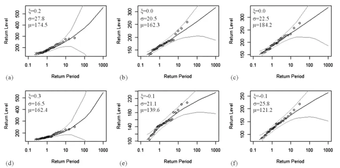
regions of the Brazilian Amazon: (a) R1, (b) R2, (c) R3, (d) R4, (e) R5 and (f) R6... 41 Figure 4.4 Return period of intense precipitation events with its respective
parameters GEV ( , and
), for homogeneous rainfall regions of the Brazilian Amazon: (a) R1, (b) R2, (c) R3, (d) R4, (e) R5 and (f) R6. The grays lines represent 95% confidence intervals and the central black line is the estimated model. The open circles are observed values... 42 Figure 4.5 Return period of intense precipitation events with its respectiveparameters GPD ( and
) and thresholds (u), for homogeneous rainfall regions of the Brazilian Amazon: (a) R1, (b) R2, (c) R3, (d) R4, (e) R5 and (f) R6. The grays lines represent 95% confidence intervals and the central black line is the estimated model. The open circles are observed values... 42 Figure 4.6 Quantile-quantile plot for the fit of GEV distribution for homogeneousrainfall regions of the Brazilian Amazon: (a) R1, (b) R2, (c) R3, (d) R4, (e) R5 and (f) R6... 44 Figure 4.7 Quantile-quantile plot for the fit of GPD for homogeneous rainfall
regions of the Brazilian Amazon: (a) R1, (b) R2, (c) R3, (d) R4, (e) R5 and (f) R6... 44 Figure 5.1 Spatial distribution of stations used in this study, for the six rainfall
homogeneous sub-regions of the Brazilian Amazon…... 51 Figure 5.2 Box plot of precipitation extremes used in the GEV and GPD
quartiles are at the ends of the box and the median is in the middle of the box. The whiskers represent the minimum and maximum values unless there are outliers. The individual circles represent the outliers.... 55 Figure 5.3 Return period of intense precipitation events with its respective
parameters GEV (, and
), in the austral summer for homogeneous rainfall regions of the Brazilian Amazon: (a) R1, (b) R2, (c) R3, (d) R4, (e) R5 and (f) R6. The grays lines represent 95% confidence intervals and the central black line is the estimated model. The open circles are observed values... 59 Figure 5.4 Return period of intense precipitation events with its respectiveparameters GEV ( , and
), in the austral autumn for homogeneous rainfall regions of the Brazilian Amazon: (a) R1, (b) R2, (c) R3, (d) R4, (e) R5 and (f) R6. The grays lines represent 95% confidence intervals and the central black line is the estimated model. The open circles are observed values... 59 Figure 5.5 Return period of intense precipitation events with its respectiveparameters GEV (, and
), in the austral winter for homogeneous rainfall regions of the Brazilian Amazon: (a) R1, (b) R2, (c) R3, (d) R4, (e) R5 and (f) R6. The grays lines represent 95% confidence intervals and the central black line is the estimated model. The open circles are observed values... 60 Figure 5.6 Return period of intense precipitation events with its respectiveparameters GEV ( , and ), in the austral spring for homogeneous rainfall regions of the Brazilian Amazon: (a) R1, (b) R2, (c) R3, (d) R4, (e) R5 and (f) R6. The grays lines represent 95% confidence intervals and the central black line is the estimated model. The open circles are observed values... 60 Figure 5.7 Return period of intense precipitation events with its respective
confidence intervals and the central black line is the estimated model. The open circles are observed values... 62 Figure 5.8 Return period of intense precipitation events with its respective
parameters GPD ( and ) and threshold ( u ), in the austral autumn for homogeneous rainfall regions of the Brazilian Amazon: (a) R1, (b) R2, (c) R3, (d) R4, (e) R5 and (f) R6. The grays lines represent 95% confidence intervals and the central black line is the estimated model. The open circles are observed values... 62 Figure 5.9 Return period of intense precipitation events with its respective
parameters GPD ( and
) and threshold ( u ), in the austral winter for homogeneous rainfall regions of the Brazilian Amazon: (a) R1, (b) R2, (c) R3, (d) R4, (e) R5 and (f) R6. The grays lines represent 95% confidence intervals and the central black line is the estimated model. The open circles are observed values... 63 Figure 5.10 Return period of intense precipitation events with its respectiveparameters GPD ( and
) and threshold ( u ), in the austral spring for homogeneous rainfall regions of the Brazilian Amazon: (a) R1, (b) R2, (c) R3, (d) R4, (e) R5 and (f) R6. The grays lines represent 95% confidence intervals and the central black line is the estimated model. The open circles are observed values... 63 Figure 6.1 Spatial distribution of stations used in this study, for the six rainfallhomogeneous sub-regions of the Brazilian Amazon... 69 Figure 6.2 (a) Number of cases selected in each region: South (R1R2), Coast
(R3R4) and Northwest (R5R6), and (b) Percentage of the number of cases separated by season of the year... 71 Figure 6.3 Composition of anomalies for the south of the Amazon at 850hPa, in
the austral summer (DJF), for D(-6), D(-3) and D(0): (a) geopotential anomalies (gpm, interval of 50 gpm), (b) current lines and vector winds anomalies, (c) Moisture convergence (105g/kg.s). The shaded areas are significant at the level of 95%... 73 Figure 6.4 Composition of anomalies for the coast of the Amazon region at
geopotential anomalies (gpm, interval of 50 gpm), (b) current lines and vector winds anomalies, (c) Moisture convergence (105g/kg.s). The shaded areas are significant at the level of 95%... 74 Figure 6.5 Composition of anomalies for the the northwest of the Amazon region
of the Amazon at 850hPa, in the austral winter (JJA), for D(-6), D(-3) and D(0): (a) geopotential anomalies (gpm, interval of 50 gpm), (b) current lines and vector winds anomalies, (c) Moisture convergence (105g/kg.s). The shaded areas are significant at the level of 95%... 76 Figure 6.6 Composition of anomalies for the south of the Amazon at 500hPa, in
the austral summer (DJF), for D(-6), D(-3) and D(0): (a) geopotential anomalies (gpm, interval of 150 gpm) and (b) omega anomalies (Pa/s, interval of 0.03 Pa/s) ... 77
Figure 6.7 Composition of anomalies for the coast of the Amazon at 500hPa, in the austral autumn (MAM), for D(-6), D(-3) and D(0): (a) geopotential anomalies (gpm, interval of 150 gpm) and (b) omega anomalies (Pa/s, interval of 0.03 Pa/s) ... 78
Figure 6.8 Composition of anomalies for the northwest of the Amazon at 500hPa, in the austral winter (JJA), for D(-6), D(-3) and D(0): (a) geopotential anomalies (gpm, interval of 150 gpm) and (b) omega anomalies (Pa/s, interval of 0.03 Pa/s) ... 79
Figure 6.9 Composition of anomalies for the south of the Amazon at 200hPa, in the austral summer (DJF), for D(-6), D(-3) and D(0): (a) geopotential anomalies (gpm, interval of 200 gpm), (b) current lines and vector winds anomalies... 80
Figure 6.10 Composition of anomalies for the coast of the Amazon at 200hPa, in the austral autumn (MAM), for D(-6), D(-3) and D(0): (a) geopotential anomalies (gpm, interval of 200 gpm), (b) current lines and vector winds anomalies... 81
LISTA DE TABELAS
Pag.
Tabela 2.1 Número de estações por estado e suas respectivas porcentagens de falhas... 6 Tabela 2.2 Modelo de construção das séries sintéticas... 10 Table 4.1 Estimative of return period of intense precipitation events (mm) for the
six sub-regions of the Brazilian Amazon, for different return period (in years), obtained through GEV and GPD distributions... 43 Table 4.2 Results of the KS test (at 5% significance level) to verify the quality of
the adjust of GEV and GPD distributions to the intense precipitation events for the homogeneous rainfall regions of the Brazilian Amazon... 45 Table 5.1 Results of the Kolmogorov-Smirnov test to check the quality of fit of the
GEV and GPD distributions to the intense precipitation events, for
Brazilian Amazon regions with homogeneous rainfall, in the four
LISTA DE SIGLAS E ABREVIATURAS EM PORTUGUÊS ANA BDMEP EPI IC INMET IS LI SUDAM TVE ZCAS ZCIT
Agência Nacional de Água
Banco de Dados Meteorológicos para Ensino e Pesquisa Eventos de Precipitação Intensa
Intervalo de Confiança
Instituto Nacional de Meteorologia Índice Silhouette
Linhas de Instabilidade
Superintendência de Desenvolvimento da Amazônia Teoria dos Valores Extremos
Zona de Convergência do Atlântico Sul Zona de Convergência Intertropical
EM INGLÊS BH CI CSL DJF ECMWF EVT GEV GPD HLCV IPE ITCZ JJA KS MAM SACZ SAMS SI SJS Bolivian High Confidence intervals Coastal Squall Lines
December, January and February
European Centre for Medium-Range Weather Forecasts Extreme Values Theory
Generalized Extreme Value Generalized Pareto Distribution High Level Cyclonic Vortices Intense Precipitation Events Intertropical Convergence Zone June, July and August
Kolmogorov-Smirnov March, April and May
South Atlantic Convergence Zone South American Monsoon System Silhouette Index
SON SST WMO
September, October and November Sea Surface Temperatures
CAPÍTULO 1
INTRODUÇÃO
A Amazônia Brasileira localiza-se na região equatorial entre 5°N-18°S e 42°W-74°W. Envolve nove estados, todos os sete da região Norte (Acre, Amapá, Amazonas, Pará, Rondônia, Roraima e Tocantins), um do Centro-Oeste (Mato Grosso), e um do Nordeste (parte do estado do Maranhão, a oeste do meridiano de 44º), totalizando uma área de aproximadamente 5.217.423 km2 correspondente a cerca de 61% do território Brasileiro (de acordo com a Superintendência de Desenvolvimento da Amazônia - SUDAM). Devido a sua grande extensão territorial esta região apresenta diferentes características meteorológicas e climáticas. Essas diferenças estão relacionadas a efeitos topográficos e à presença de sistemas meteorológicos que atuam em diferentes escalas de tempo. Além disso, são modulados por mecanismos de interação na interface oceano-atmosfera, que podem promover totais pluviométricos acima e/ou abaixo da média climatológica (De Souza et al., 2005).
Dentre os sistemas meteorológicos de escala sinótica que condicionam o regime pluviométrico na Amazônia, os principais são: Zona de Convergência Intertropical (ZCIT) e Zona de Convergência do Atlântico Sul (ZCAS). A ZCIT é parte integrante da circulação geral da atmosfera e forma-se dentro do ramo ascendente da célula de Hadley, na região de confluência dos ventos alísios de nordeste (procedentes do hemisfério norte) com os de sudeste (procedentes do hemisfério sul), originados dos anticiclones subtropicais do Atlântico Norte e do Atlântico Sul. É uma região de baixa pressão atmosférica, de convecção profunda e intensa nebulosidade, associada com altos valores pluviométricos (Hastenrath, 1985; Curtis e Hastenrath, 1999), responsável pelo máximo de precipitação durante o outono austral no hemisfério sul (De Souza et al., 2005; De Souza e Rocha, 2006). A ZCAS atua principalmente na região sul e sudoeste da Amazônia, responsável pelo máximo de precipitação no final da primavera e verão austral (Carvalho et al., 2004; Grimm, 2011; De Oliveira Vieira et al., 2013; Quadro et al., 2012). Sua principal característica é a alta variabilidade convectiva posicionada a leste da Cordilheira dos Andes com orientação noroeste-sudeste, desde o sul da Amazônia até o Atlântico Sul (Carvalho et al., 2002; 2004).
de friagem. Este fenômeno ocasiona uma brusca alteração nas condições meteorológicas, causando uma diminuição da temperatura e umidade do ar, modificando as características ambientais. Normalmente, as friagens estão relacionadas ao desenvolvimento de um anticiclone atrás de um sistema frontal que se move para o norte, atingindo a região da Amazônia (Hamilton e Tarifa, 1978; Marengo et al., 1997).
Quanto aos sistemas de mesoescala destacam-se as Linhas de Instabilidade (LI), que formam-se ao longo da costa norte e nordeste da América do Sul, associada à circulação de brisa marítima, sendo mais frequente no inverno e outono austral (Cohen et al., 1995; Alcântara et al., 2011). Algumas destas LI propagam-se para o interior da bacia Amazônica e outras dissipam-se próximo à costa atlântica (Silva Dias e Ferreira, 1992; Cohen et al., 1995). A topografia e a circulação local também são importantes nessa região, podendo aumentar a atividade dos sistemas convectivos, que sob condições atmosféricas favoráveis podem gerar forte precipitação e tempo severo em poucas horas (Smith et al. 1996).
A Amazônia vem sendo atingida por diversos eventos extremos de precipitação, tanto com períodos prolongados com e sem chuva, quanto com o aumento dos eventos com chuvas intensas. Segundo Gloor et al. (2013), desde o final do século XX (começando aproximadamente em 1990), houve uma grande intensificação do ciclo hidrológico amazônico, com um aumento do deságue durante a estação chuvosa e eventuais secas severas. Brito et al. (2014) estudaram diferentes tipos de eventos extremos de precipitação na Amazônia, analisando frequência, intensidade e a contribuição para a climatologia da precipitação acumulada, para o período de 1998 a 2013, e observaram que os extremos de precipitação produziram mais chuvas nos últimos sete anos, atingindo um máximo durante 2011-2012.
Diante do exposto, conhecer o período de retorno dos Eventos de Precipitação Intensa (EPI) é de vital importância para o planejamento das atividades sujeitas a seus efeitos adversos. Uma forma de estimar esses eventos é através da Teoria dos Valores Extremos (TVE), que concentra-se em classes especiais de distribuições de probabilidade: Distribuição Generalizada de Valores Extremos (Generalized Extreme Value - GEV), que inclui as distribuições de Gumbel, de Fréchet e de Weibull, e a Distribuição Generalizada de Pareto (Generalized Pareto Distribution - GPD), como a Exponencial, a Pareto e a Beta. Neste trabalho, as duas distribuições (GEV e GPD) foram usadas.
1.1Problema, Motivação e Hipótese
Os EPI vêm causando grandes prejuízos sociais e econômicos às regiões atingidas, principalmente em cidades cuja infraestrutura não é adequada para evitar enchentes e aquelas que possuem habitações em locais de risco, como encostas de montanhas, vales de rios e córregos. Na Amazônia, os EPI causam consequências negativas especificamente aos núcleos de ocupação populacional nas margens dos seus inúmeros rios, pois as enchentes e inundações impossibilitam o cultivo de plantações e, dificultam inclusive a saída e o acesso às comunidades para a obtenção de mantimentos e de receber ajuda governamental.
Investigações científicas no âmbito da modelagem climática sugerem que as mudanças no clima atual estão resultando em EPI mais frequentes e que a interferência do homem no meio ambiente vem intensificando as consequências destes eventos, com ações como o desmatamento de encostas e a construção civil em áreas de risco (Marengo, 2009(b)). Em 2014, dois estados, Acre e Rondônia, decretaram estado de calamidade pública devido às inundações causadas por chuvas fortes nas nascentes de seus rios.
Diante do exposto, a motivação para a realização deste estudo está na necessidade de um melhor entendimento do comportamento dos EPI, conhecer o período de retorno desses eventos, no sentido de proporcionar uma previsão de melhor qualidade e minimizar os prejuízos causados à população. Além da importância de estimar o período de retorno dos EPI, também é importante conhecer os fatores que antecedem sua formação, ou seja, conhecer os padrões atmosféricos dominantes na ocorrência dos EPI, que são essenciais para o monitoramento climático e previsão do tempo e, podem ser usados como fonte de informação para ações de cunho social e econômico.
i) Quantas sub-regiões são suficientes para representar regiões pluviometricamente homogêneas na Amazônia Brasileira?
ii) Qual o período e nível de retorno dos EPI nas sub-regiões da Amazônia Brasileira?
iii) Quais regiões e período (estação do ano) apresentam os maiores EPI?
iv) Quais são os padrões atmosféricos dominantes na ocorrência dos EPI?
As hipóteses para responder a essas questões são:
i) Visto que no sul da Amazônia o principal sistema produtor de chuva é a ZCAS e no Norte são ZCIT e LI, então é esperado que duas sub-regiões (Norte e Sul) sejam suficientes para representar regiões pluviometricamente homogêneas na Amazônia Brasileira.
ii) Uma vez que resultados de estudos utilizando modelagem climática mostram alterações no ciclo hidrológico na Amazônia, então é possível que os EPI apresentem um período de retorno curto.
iii) Investigações científicas sugerem que a interferência do homem no meio ambiente vem intensificando as consequências dos EPI, então espera-se que os EPI de maior impacto possam estar ocorrendo nas regiões mais afetadas pela ação do homem, como por exemplo, nas regiões do arco do desmatamento. Quanto ao período, possivelmente seja na estação chuvosa da região encontrado os maiores EPI. Pois, a atuação simultânea, ou não, dos sistemas meteorológicos e seus posicionamentos relativos à região, muitas vezes são os responsáveis pelos eventos extremos de precipitação.
iv) Os padrões de circulação predominantes variam ao longo do ano e espera-se que em função desta variação seja possível explicar os EPI.
1.2Objetivos
O objetivo geral desta pesquisa é estudar os EPI, com aplicação da TVE para estimar o período de retorno desses eventos e identificar as regiões da Amazônia Brasileira onde ocorrem os EPI de maior relevância.
Os objetivos específicos são:
Determinar regiões homogêneas com base nas normais climatológicas de precipitações, e associá-las aos principais sistemas atmosféricos que atuam na região.
Estimar o período e nível de retorno dos EPI nas sub-regiões da Amazônia Brasileira, através da TVE;
Indicar as regiões e o período (estação do ano) com EPI de maior relevância;
Estabelecer características dos padrões atmosféricos dominantes na ocorrência dos EPI.
1.3Estrutura da Tese
Esta tese está organizada da seguinte forma: o Capítulo 2 apresenta uma descrição da metodologia utilizada. No Capítulo 3, com base nas normais climatológicas de precipitações, as regiões homogêneas são determinadas. O Capítulo 4 e 5 apresentam as estimativas do período de retorno dos EPI, indicando as regiões onde ocorrem EPI de maior relevância. O Capítulo 6 exibe os padrões atmosféricos dominantes na ocorrência dos EPI. Finalmente, no Capítulo 7 são apresentadas as considerações finais da tese e sugestões para trabalhos futuros. Na sequência são apresentadas as publicações que deram origem aos capítulos:
Capítulo 3 - Santos, E. B.; Lucio, P. S.; Santos e Silva, C. M. Precipitation regionalization of the Brazilian Amazon. Atmospheric Science Letters, 2014. DOI: 10.1002/asl2.535.
Qualis CAPES: A1 - Interdisciplinar/B1 - Geociências. Fator de impacto: 1.876.
Capítulo 4 - Santos, E. B.; Lucio, P. S.; Santos e Silva, C. M. Estimating return periods for daily precipitation extreme events over the Brazilian Amazon. Theoretical and Applied Climatology (em revisão).
Qualis CAPES: A2 - Interdisciplinar/A2 - Geociências. Fator de impacto: 1.742.
Capítulo 5 - Santos, E. B.; Lucio, P. S.; Santos e Silva, C. M. Seasonal analysis of return periods for maximum daily precipitation in the Brazilian Amazon. Journal of Hydrometeorology, 2015. DOI: 10.1175/JHM-D-14-0201.1.
Qualis CAPES: A2 - Interdisciplinar/A1 - Geociências. Fator de impacto: 3.573.
CAPÍTULO 2
DADOS E METODOLOGIA
2.1Dados
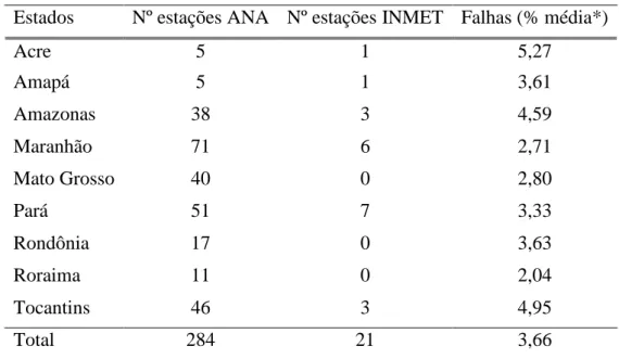
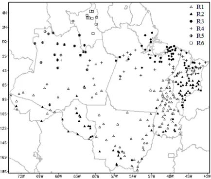
Foram utilizados os dados diários de precipitação da rede hidrometeorológica gerenciada pela Agência Nacional de Água (ANA) e do Banco de Dados Meteorológicos para Ensino e Pesquisa (BDMEP) do Instituto Nacional de Meteorologia (INMET). O conjunto inicial de dados foi composto de 1129 estações. Esses dados passaram por uma série de etapas a fim de serem organizados e analisados. As estações foram selecionadas seguindo as recomendações da Organização Meteorológica Mundial (World Meteorological Organization - WMO), estabelecidas no Documento Técnico WMO-TD/Nº. 341. Neste documento, recomenda-se descartar o mês que apresente algum valor diário faltante e séries mensais com dados faltantes em três ou mais meses consecutivos ou mais que 5 meses alternados. Após a verificação da qualidade dos dados, seguindo as recomendações da WMO, das 1129 estações recebidas foram escolhidas 305 estações (Tabela 2.1), para o período de 1983 a 2012, por ser este o período (com no mínimo 30 anos de dados) que apresentou dados mais consistentes. As estações escolhidas estão distribuídas de acordo com a Figura 2.1.
Tabela 2.1 - Número de estações por estado e suas respectivas porcentagens de falhas. Estados Nº estações ANA Nº estações INMET Falhas (% média*)
Acre 5 1 5,27
Amapá 5 1 3,61
Amazonas 38 3 4,59
Maranhão 71 6 2,71
Mato Grosso 40 0 2,80
Pará 51 7 3,33
Rondônia 17 0 3,63
Roraima 11 0 2,04
Tocantins 46 3 4,95
Total 284 21 3,66
Figura 2.1 - Distribuição espacial das 305 estações (INMET: 21 e ANA: 284) meteorológicas utilizadas.
Para caracterizar os padrões atmosféricos associados aos EPI foram utilizados os dados diários das reanálises do projeto ERA Interim (Dee et al., 2011), do European Centre for Medium-Range Weather Forecasts (ECMWF). Estes dados cobrem o período de 01 de janeiro de 1979 até a data atual e apresentam espaçamento de grade de 1,5º latitude x 1,5º longitude. As variáveis meteorológicas utilizadas são: vento zonal, vento meridional, geopotencial, velocidade vertical (ômega) e umidade específica, para o período de 1983 a 2012.
2.2Metodologia
2.2.1 Análise de Agrupamento
A análise de agrupamento, ou análise de cluster, é uma técnica multivariada que busca agrupar elementos de dados com base na similaridade entre eles. Os grupos são determinados de forma a obter-se homogeneidade dentro deles e heterogeneidade entre eles. Neste estudo, as normais climatológicas (médias históricas, compreendendo no mínimo 30 anos consecutivas) de precipitação das 305 estações foram utilizadas como variáveis para determinar regiões homogêneas de precipitação. Os totais mensais e as normais climatológicas foram calculadas seguindo as recomendações da WMO.
segundo Mimmack et al. (2001), é a uma das medidas indicadas para regionalização de dados climáticos. A distância euclidiana entre dois elementos = [ , , … , 𝑛] e =
[ , , … , 𝑛], num espaço euclidiano n-dimensional, é definida por:
2 1 2 2 2 2 2 11 ) ( ) ... ( )
(
n i i i n nxy X Y X Y X Y X Y
d (2.1)
onde Xi e Yi são os elementos a serem comparados, que nesta pesquisa são as médias mensais (normais climatológicas) de precipitação das 305 estações.
A segunda etapa é definir o método. Os métodos hierárquicos são classificados em aglomerativos e divisivos. Usamos neste estudo o hierárquico aglomerativo de Ward. No método aglomerativo, cada elemento da base representa um grupo isolado. Nas interações posteriores, cada grupo vai se unindo a outro de acordo com sua similaridade até obter o número de agrupamento desejado (Bien e Tibshirani, 2011), como pode ser observado na Figura 2.2.
Figura 2.2 - Dendograma: agrupamento hierárquico aglomerativo. Fonte: Bien e Tibshirani, 2011.
O método de Ward foi utilizado por buscar unir elementos que tornem os grupos formados o mais homogêneo possível. Este método busca a menor variância entre os agrupamentos, unindo os elementos cuja soma dos quadrados entre eles seja mínima ou que o erro desta soma seja mínimo (Hervada-Sala e Jarauta-Bragulat, 2004).
2.2.2 Índice Silhouette
O Índice Silhouette (IS), elaborado por Rousseeuw (1987), avalia o quanto uma observação é semelhante às outras observações inseridas em seu grupo, comparado com observações inseridas em outros grupos. Neste estudo, o IS foi utilizado para avaliar a qualidade dos grupos formados pela análise de agrupamento.
Os valores deste índice variam no intervalo [-1,1]. Valores próximos a 1 indicam que o objeto está no grupo correto. Valores próximos a -1 indicam que a observação foi provavelmente alocada a um grupo inadequado. Valores próximos de zero indicam que o objeto está próximo à fronteira entre dois grupos e não pertencem a um grupo ou outro. Cada observação apresenta um IS, e uma média geral de todas as observações permite avaliar o desempenho geral do agrupamento. O IS(n) é calculado de acordo com a equação (Rousseeuw, 1987):
n b n a n a n b n IS , max (2.2)sendo n a observação que está sendo avaliada, a(n) é a média das distâncias da n-ésima observação a todas as outras dentro do mesmo grupo, e b(n) é a média das distâncias dessa n-ésima observação a todas as outras alocadas no grupo mais próximo. A qualidade global do agrupamento pode ser medida por meio da média deIS
n , conforme a equação:N IS IS N n n
1 ( ) (2.3)
em que N representa o total de observações.
2.2.3 Intervalo de Confiança
O Intervalo de Confiança (IC) a 95% foi aplicado nas normais climatológicas de precipitação dos grupos. O objetivo é construir um IC para o parâmetro com uma probabilidade de 1(nível de confiança) de que o intervalo contenha o verdadeiro valor do parâmetro. Portanto, o IC foi utilizado para ajudar identificar se os elementos estão no grupo correto.
Seja XF o parâmetro de interesse, 𝜆𝑖 o limite inferior e 𝜆𝑠 o limite superior. O IC é dado pela equação:
𝑃 𝜆𝑖 < 𝐹 < 𝜆𝑠 = 1 − 𝛼 (2.4)
Considerando o IC a 95%, α é 5% que é o erro que pode ocorrer ao ser afirmado que,
2.2.4 Séries Sintéticas
Na Amazônia, a falta de dados qualificados é um dos obstáculos para a realização de estudos sobre eventos extremos de precipitação. Por isso, utilizamos séries sintéticas para representar as regiões pluviometricamente homogêneas. Visto que o objetivo do estudo é estudar EPI, essas séries foram construídas com os valores máximos diários de cada sub-região, como pode ser observado na Tabela 2.2.
Tabela 2.2 – Modelo de construção das séries sintéticas. Ano Mês Dia Estação 1
(mm)
Estação 2 (mm)
Estação 3 (mm)
Estação 4 (mm)
Série sintética (mm)
1983 1 1 12,4 49,2 85,2 7,5 85,2
1983 1 2 38,2 19,8 0 8,4 38,2
1983 1 3 8,6 7,8 10,2 0 10,2
2.2.5 Teoria dos Valores Extremos
A TVE foi aplicada nas séries temporais de precipitação diária (séries sintéticas). Esta teoria é um ramo da probabilidade para o estudo do comportamento estocástico de extremos associados a uma função de distribuição F normalmente desconhecida. O objetivo principal da TVE é estimar a cauda (superior ou inferior) de uma distribuição referente a um conjunto de observações independentes e identicamente distribuídas.
Coles (2001) demostra a formulação inicial do modelo como a seguir:
𝑀𝑛 = 𝑎𝑥{ , … , 𝑛} (2.5)
sendo 𝑀𝑛 o máximo das n unidades, e , ..., 𝑛 uma sequência de variáveis aleatórias independentes e identicamente distribuídas com distribuição acumulada F em comum.
Nesta teoria, a distribuição dos valores de 𝑀𝑛 pode ser obtida para todos os valores de n, da seguinte forma:
𝐹𝑀𝑛 𝑧 = 𝑃 𝑀𝑛 ≤ 𝑧 = 𝑃 ≤ 𝑧, … , 𝑛 ≤ 𝑧 = {𝐹 𝑧 }𝑛 (2.6)
A mesma teoria também pode ser aplicada para a previsão de eventos extremos mínimos. Nesse caso a formulação é representada por:
𝑀𝑛 = 𝑖 { , … , 𝑛} (2.7)
sendo 𝑀𝑛 o mínimo das n unidades, e , ..., 𝑛 a sequência de variáveis independentes com distribuição F em comum.
Para garantir a independência das séries temporais de precipitação diária (séries sintéticas), os dados foram randomizados, removendo a dependência sazonal, ou seja, se os EPI ocorreram em apenas uma estação do ano, com a randomização esses eventos se tornam aleatórios. Para verificar a hipótese de independência dos dados, foi utilizado o teste não paramétrico de sequências (runs tests), que verifica se os elementos da série são mutuamente independentes. Adotou-se 5% como nível de significância para o teste.
2.2.5.1Distribuição Generalizada de Valores Extremos
A distribuição GEV combina as três formas assintóticas de distribuição de valores extremos, Gumbel, Weibull e Fréchet (Fisher e Tippett, 1928), em uma única forma, definida segundo Jenkinson (1955), como a seguir:
1 1 exp )
(x x
F , para 0
(2.8) x x
F( ) exp exp , para 0
(2.9)
sendo
o parâmetro de posição com
;
é um parâmetro de escala com
0 e é um parâmetro de forma com .
As distribuições de valores extremos de Weibull e de Fréchet correspondem aos casos particulares de (2.8) em que 0 e 0, respectivamente. Quando 0, a função assume a forma (2.9), que representa a distribuição de Gumbel.
Para o quantil
x
P da distribuição GEV, com o período de retorno T, a probabilidade acumulada é dada por 𝐹 𝑥𝑝 = 1 − 1/T , que resulta em (Palutikof et al., 1999): T
xp 1 ln 1 1 , para 0
T
xp ln ln 1 1 , para 0
(2.11)
Na distribuição GEV, a base de dados final foi determinada conforme a metodologia block maxima ou máximos anuais (Gumbel) (Maraun et al., 2009; Sugahara et al., 2009), onde a amostra é dividida em subperíodos (blocos) que podem ser mensais, anuais, etc. De cada bloco, extrai-se o valor máximo ou mínimo, para formar o conjunto de eventos extremos. Na Figura 2.3, as observações
x
2, x
5 ex
11, representam os máximos para três blocos com períodos de quatro observações. Esse procedimento apresenta a desvantagem da possibilidade de perder possíveis eventos extremos dentro do mesmo bloco. Observa-se na Figura 2.3, que no terceiro bloco foi desconsiderado um valor maior que os máximosx
2 ex
5.Figura 2.3 - Representação dos eventos extremos para distribuição GEV.
2.2.5.2Distribuição Generalizada de Pareto
Pickands (1975) mostrou que a distribuição assintótica dos excessos de uma variável aleatória acima de um valor limiar pode ser aproximada por meio da GPD. Assim como na distribuição GEV, a GPD pode ser interpretada como uma família de distribuições, que dependendo do valor do parâmetro de forma, inclui casos particulares, definida como:
1 1 1 x u
x
F , para 0
(2.12)
u x xF 1 exp , para 0
(2.13)
em que
u
é o limiar selecionado, ou seja, os valores dex
u
são os excedentes. Para 0, a GPD é uma distribuição Exponencial. Para 0, a GPD é uma distribuição Pareto, e para0
O quantil
x
P da distribuição GPD, será obtido como segue (Abild et al., 1992; Palutikof et al., 1999):
u
T
x
p1
, para 0(2.14)
)
ln( T
u
x
p
, para 0 (2.15)sendo
igual a Mn
, onde
n
é o número total de valores excedentes acima do limiaru
e M é o número de anos do registro.Na GPD, a base de dados final foi determinada conforme a metodologia peaks over threshold (Sugahara et al., 2009), que considera apenas os valores acima de um limiar estabelecido. Na Figura 2.4, as observações
x
2,
x
3,
x
5,
x
7,
x
8,
x
11 ex
12, excedem o limiaru
e constituem os eventos extremos.Figura 2.4 - Representação dos eventos extremos para GPD.
Nos gráficos das médias residuais, como pode ser observado na Figura 2.5, a mudança de inclinação indica diferentes parâmetros para a distribuição dos excedentes e o comportamento irregular na parte direita do gráfico é devido ao pequeno número de excedentes acima de altos limiares. Na figura 2.5, a média dos resíduos apresenta maior variação a partir do limiar 100, o que pode ser interpretado como um ponto de partida para avaliação do limiar adequado para a modelagem dos eventos extremos.
Figura 2.5 – Média Residual de dados diários de precipitação.
2.2.5.3Estimação dos Parâmetros
Os parâmetros das distribuições GEV (
,
e ) e GPD (
e ) foram calculados utilizando o método de máxima verossimilhança (Smith, 1985), que consiste basicamente em maximizar uma função dos parâmetros da distribuição, conhecida como função verossimilhança.Seja
x
1,
x
2,...,
x
n
uma amostra de n valores de uma distribuição de parâmetros
p p pk
p 1, 2,..., e função densidade de probabilidade f
xi | p . A função de verossimilhança de X com relação à amostra é dada por:
n i
i p
x f P
L
1
| (2.16)
Os estimadores p'
p'1,p'2,...,p'k
do conjunto de parâmetros pde f
xi | p são aqueles que maximizam a função de verossimilhança L
p .2.2.6 Teste Kolmogorov-Smirnov
A qualidade do ajuste das distribuições GEV e GPD foi verificada através do teste Kolmogorov-Smirnov (KS). Adotou-se 5% como nível de significância para o teste.
limite superior extremo das diferenças entre os valores absolutos da distribuição acumulada empírica e teórica consideradas no teste (Lucio, 2004). F
x é a função de distribuição acumulada teórica, e G
x é a função de distribuição acumulada empírica, para n observações aleatórias com uma função de distribuição acumulada. A hipótese nula é rejeitada se o valor den
D for maior que o valor tabelado. Isso equivale a considerar que a probabilidade exata do teste
é menor que o nível de significância.
2.2.7 Composição de Anamalias
Após selecionado os EPI, com base no cálculo dos percentis da distribuição de precipitação e outros critérios (descrito no Capítulo 6), campos de composições das anomalias de geopotencial, vento e velocidade vertical (ômega) foram calculados, para o dia do evento-D(0), três-D(-3) e seis-(D-6) dias precedentes. Além das anomalias dessas variáveis, foi calculada a composição da divergência do fluxo de umidade, onde os valores negativos indicam convergência de umidade e os valores positivos indicam divergência de umidade. Neste estudo, foram plotados apenas os valores de convergência e multiplicados por -1.
A técnica de composição foi utilizada por ser eficiente em identificar os padrões médios e as principais características associadas a um determinado fenômeno meteorológico. O cálculo dos campos de composições de anomalias das variáveis foi obtido de maneira semelhante a Lima et al. (2010) e Lima e Satyamurty (2010), como segue:
N i j n D j z y x N n D z yx, , , 1 , , , , (2.17)
onde
é a variável do composto, (x,y,z) indica a posição espacial da variável, N é o número de casos identificados durante o período de estudo, D-n é o nésimo dia precedente ao evento (n=0,1,2,3) e o sufixo j refere-se ao jésimo evento.Considerando cx,y,z a climatologia da variável
, os campos da anomalia dacomposição
AC serão obtidos da seguinte maneira:
x y z D n
x y z D n
c
x y z
AC , , , , , , , ,
(2.18)
N t
AC
. % 95
(2.19)
Para a composição de anomalia (
AC) ser aceita ao nível de significância de 5%, a mesma tem que ser maior ou igual aN t95%.
Santos, E. B.; Lucio, P. S.; Santos e Silva, C. M. Precipitation regionalization of the Brazilian Amazon. Atmospheric Science Letters, 2014. DOI: 10.1002/asl2.535.
CAPÍTULO 3
PRECIPITATION REGIONALIZATION OF THE BRAZILIAN AMAZON (Regionalização da precipitação na Amazônia Brasileira)
RESUMO
A Amazônia Brasileira possui uma grande extensão territorial, onde atuam diferentes sistemas atmosféricos, os quais contribuem para a não homogeneidade pluviométrica da região. Neste sentido, o objetivo deste estudo é determinar regiões homogêneas de precipitação na Amazônia Brasileira, associando-as aos principais sistemas atmosféricos que atuam na região. Com esta finalidade, a análise de agrupamento hierárquica foi aplicada em um conjunto de dados pluviométricos de 305 estações. Os resultados sugerem que a Amazônia Brasileira possui seis regiões pluviometricamente homogêneas.
ABSTRACT
The Brazilian Amazon is a large territory, where different weather systems act, contributing to non-homogeneity of the rainfall seasonal distribution in the region. The aim of this study is to determine sub-regions of homogeneous precipitation in the Amazon, linking them to the main atmospheric systems that affect the rainfall in the region. For this, hierarchical cluster analysis was applied on a data set composed by 305 rain gauges. The results suggest that the Brazilian Amazon has six pluvial homogeneous regions.
3.1Introduction
The Brazilian Amazon is located in the equatorial region between 5°N-18°S and 42ºW-74ºW, and it is characterized by having a moist atmosphere with large and intense convective activity due to the diabatic heating from the solar energy throughout the year in association with mechanisms, such as the Intertropical Convergence Zone (ITCZ) migration, Coastal Squall Lines (CSL) propagation, and others. The climate of this region is determined by a combination of various physical and dynamical processes of large-scale, as well as local features, which are responsible for temporal and spatial distribution of precipitation.
Among the synoptic scale weather systems that affect the rainfall in the Amazon, the main ones are: i) ITCZ, responsible for the maximum rainfall during the austral autumn (De Souza et al., 2005; De Souza and Rocha, 2006). ii) the South Atlantic Convergence Zone (SACZ), acting mainly in the south and southwestern Amazon region, responsible for the maximum rainfall in late spring and austral summer (Carvalho et al., 2004; Grimm, 2011; De Oliveira Vieira et al., 2013) and iii) the Bolivian High (BH), which also contributes for the precipitation during the austral summer (Figueroa et al., 1995; Lenters and Cook, 1997). During the austral winter, the migration of the ITCZ to the northern hemisphere and the weakening of BH change the intensity and distribution of precipitation in the Amazon. During the austral winter, surges of cold high-latitude air, known locally as “friagens”, move across southeastern Brazil and Amazonia from the south, greatly modifying the atmospheric structure and climatic conditions. The characteristics of this phenomenon are more easily detected at stations southwest of the Amazon (Marengo et al., 1997, Longo et al., 2004).
The main mesoscale system that acts in the region is the CSL (Cohen et al., 1995), which are formed along the northern coast of South America, associated with sea breeze circulation, more frequent between April and June and less frequent between October and November (Alcântara et al., 2011). The propagation of CSL modulates the diurnal cycle of precipitation, which is characterized by strongest rainfall rate between 1400 and 1800 HL (Santos e Silva et al., 2012). Furthermore, the local wind mechanisms, such as river breeze are also important to the diurnal cycle and intensity of rainfall in this region (Oliveira and Fitzjarrald, 1993; Silva Dias et al., 2004).
3.2Material and Methods
3.2.1 Datasets
Daily rainfall dataset was obtained from National Water Agency (Agência Nacional de Água - ANA) and Meteorological Database for Education and Research (Banco de Dados Meteorológicos para Ensino e Pesquisa - BDMEP) of the National Institute of Meteorology (Instituto Nacional de Meteorologia - INMET). The total monthly and normal climatological rainfall (average monthly rainfall) were calculated following the recommendations of the World Meteorological Organization (WMO), established in Technical Document WMO-TD / N°.341, for the period from 1983 to 2012. In this document it is recommended: i) to discard the month that show any missing daily value; ii) excluded of the climatological normal the monthly data that present 3 or more consecutive days of missing observations or more than five alternate months missing. The initial set consisted of 1,129 rain gauges, but after applying the WMO recommended procedure, 305 rain gauges were selected.
3.2.2 Methods
The climatological normal of the 305 stations were used as attributes to characterize the homogeneous regions by means of cluster analysis, a multivariate technique that searches for data elements based on the similarity between them. The clusters are determined so as to obtain homogeneity within them and heterogeneity between them.
The first stage of the clustering process is the estimation of a measure of similarity (or dissimilarity). In this work, the Euclidean distance was used, which according Mimmack et al. (2001) is one of the measures listed for regionalization of climate data. The Euclidean distance between two elements = [ , , … , 𝑛] and = [ , , … , 𝑛], an n-dimensional Euclidean space, is defined by:
21 2 2 2 2 2 1
1 ) ( ) ... ( )
(
n i i i n nxy X Y X Y X Y X Y
d
(3.1)
where
X
i andY
i are the elements to be compared, which in this study are the monthly average rainfall (climatological normal).Through prior knowledge about the data structure, a distance cutoff was determined to define which clusters will be formed.
The quality of the formed clusters was assessed using the Silhouette Index (SI), developed by Rousseeuw (1987), which evaluates how an observation is similar to other observations inserted in its cluster, compared with inserted observations in other clusters. Each observation has an SI and an overall average of all observations allows us to evaluate the overall performance of the cluster. This index ranges from -1 to 1.Values close to 1 indicate that the object is in the correct cluster. Values close to -1 indicates that the observation was probably allocated to an inappropriate cluster. Values near zero indicate that the object is close to the boundary between two clusters and do not belong to one cluster or another. The SI
n is calculated according to the equation (Rousseeuw, 1987):
n b n a n a n b n SI , max (3.2)with the observation being evaluated, a(n) is the mean distance of the n-th observation to all others within the same cluster, b(n) is the average distance that n-th observation to all other allocated in the closest cluster. The overall quality of the cluster can be measured by the average SI(n), according to the equation:
N SI SI N n n
1 ( )
(3.3)
where N is the total number of observations.
Confidence Intervals (CI) to the 95% quantile of the climatological normal were constructed and applied. The objective of estimating quantile's intervals is to build a CI for the parameter with a probability of 1 (Confidence level) that the interval contains the true parameter. Be XFthe parameter of interest, 𝜆𝑖 the lower limit and 𝜆𝑠 the upper limit. The CI is given by the equation:
𝑃 𝜆𝑖 < 𝐹 < 𝜆𝑠 = 1 − 𝛼 (3.4)
3.3Results and Discussion
In the formation of two sub-regions (Figure 3.1), the Brazilian Amazon was split into south (Region 1) and north (Region 2) which was expected, since the main rain-producing systems of the north and south of the Amazon are different. In the south, the main systems are SACZ and BH and in northern Amazon are ITCZ and CSL. Another important precipitation process in the Amazon, especially in the north, is the radiative surface heating, which can generate cells and convective clusters typical of tropical regions (Strong et al., 2005).
Figure 3.1 - Analysis of grouping to two sub-regions: (a) spatial distribution of stations; (b) SI graph; and (c) and (d) precipitation climatological normals (grey lines) of the stations belonging to the regions 1 and 2, respectively. The dotted blue lines represent the CI.
Amazon) exhibited a low SI (0.22), so the rainfall climatological normals in this region showed different patterns and some stations were outside the CI. As the length of the CI is associated with the accuracy, the smaller the length more accurate is the average. Note that the length of the CI in region 2 is much larger than the region 1, confirming that region 2 does not represent a homogeneous rainfall region.
Agreeing with some studies (Rao and Hada, 1990; Liebmann and Marengo, 2001; Marengo and Nobre, 2009; Reboita et al., 2010), that analyzed the mean annual cycle of rainfall in Amazonia, more than two sub-regions are required to represent patterns of precipitation in this region. According to Liebmann and Marengo (2001), the annual mean precipitation in the Brazilian Amazon varies by more than 50% within Brazilian Amazonia, ranging from less than 2000 mm in the south, east, and extreme north, to more than 3000 mm in the northwest, where orographic uplift begins to operate. A secondary maximum was also observed near the mouth of the Amazon River, which is associated with nighttime convergence of the easterly trades with the land breeze. With three sub-regions (Figure 3.2), the northern Amazon region was divided into two (coastal zone and northwest Amazon) and the south remained the same. The subdivision in northern Amazon is consistent with the systems operating in the region. In the coastal area of north Amazon the precipitation is associated to sea breeze, and local convection. In addition, the trade winds can intensifying the sea breeze and contribute to CSL formation that can propagates ~2,000 km into the Amazon basin (Cohen et al., 1995; Santos e Silva, 2013). The sub-regions of the north, coastal zone (region 2 in Figure 3.2) and northwestern Amazon (region 3 in Figure 3.2) show different patterns, so do not belong to the same .The coastal area of the Amazon has maximum rainfall in the first half of the year and a dry period in the second half, while the northwestern Amazon has annual maximum in austral winter and a reduction in the austral summer, but does not have a well-defined dry season. In Figure 3.2(b), it is noticed that the formation of the SI three sub-regions showed better results where the lowest SI was 0.3. In the SI it can also be seen a better result, because the lengths of the CI were lower and there was a decrease in the amount of stations outside the SI.
Figure 3.2 - Analysis of clustering to three sub-regions: (a) spatial distribution of stations; (b) SI graph; and (c), (d), and (e) precipitation climatological normals (grey lines) of the stations belonging to the regions 1, 2, and 3, respectively. The dotted blue lines represent the CI.
contributed to the state of the atmosphere during the time scale of several weeks, with distinguishable patterns of temperature, humidity, and rainfall. With regard to the types of vegetation, it is noticed that most of the region 2 in Figure 3.3 (driest region of the Brazilian Amazon) stations are in the cerrado, such as southern Maranhão. In the area of native forest (region 1 in Figure 3.3), it is noticed that the rainy season starts earlier and lasts longer than in the transition (cerrado) region, which is characterized by the region 2 in Figure 3.3.
These results are consistent with some studies that use climate models to simulate climate change caused by deforestation of the Amazon, which found that the average rainfall decreases with increasing deforestation, and distribution of rainfall is affected by the type of surface coverage as well as by the topography. While in deforested areas of the region an important decrease in precipitation occurs, the areas around these and the higher regions receive more rainfall (Ramos da Silva and Avissar, 2006; Ramos da Silva et al., 2008). However, we did not perform statistic analysis in order to verify the relationship between deforestation and rainfall over these regions to the studied period (1983-2012). In this sense, the precipitation variability in the sub-regions 1 and 2 can also be attributed to natural factor such as topography. Similarly to the formation of the four sub-regions, the next sub-regions have been separated due to having distinct precipitation intensity. For five sub-regions, the region that was subdivided was the coastal of the Amazon (forming regions 3 and 4 in Figure 3.4).These sub-regions showed the same patterns, but with different precipitation intensities. Region 3 (Figure 3.4(e)) has stations nearer to the coast and with that in these regions the rainfall is higher due to the influence of CSL that are formed along the coastline. The stations in region 4 (Figure 3.4(f)) are furthest from the coastline, and as not all CSL propagate towards the inside of the Amazon, precipitation in this region will be of lower intensity compared to region 3 (Figure 3.4(e)).
In the formation of six sub-regions, the region that was subdivided was the northwestern Amazon (forming regions 5 and 6 of Figure 3.5). The region 6 consists of stations in the State of Roraima, all from the northern hemisphere. This region has climatic characteristics of the northern hemisphere, with annual maximum in austral winter, as observed by Rao and Hada (1990) and Reboita et al. (2010). In turn, the region 5 (region of northwest and north-northwest of the State of Amazonas) has high precipitation throughout the year, showing absence of dry season.
The best SI (0.45) was found in three sub-regions; however, we observed that to characterize the overall rainfall variability in Amazon basin six sub-regions are necessary. In addition with six sub-regions, both profile and intensity of rainfall are distinguished.
In the SI it is noticed that as the number of sub-regions increased, fewer stations are outside of the SI, and the lengths of these intervals decreased, thereby increasing the accuracy of the results.
3.4Conclusions
The large territory and varied landforms of the Amazon allow the development and performance of different weather systems that contribute to the existence of at least three rainfall homogeneous sub-regions, associated systems: ITCZ, SACZ, BH and CSL.
These results suggest that three sub-regions are sufficient to separate the Brazilian Amazon in different patterns of precipitation, but in more detailed studies, the ideal is to use the six sub-regions, which are separated considering distinct rainfall intensity.
All sub-regions formed by agglomerative hierarchical Ward method are consistent with the performance of the main weather systems of precipitation generators and/or local conditions in the region. Local conditions contribute mainly in separating sub-regions considering the intensity of precipitation.
The results may serve to help in the analysis and weather forecasts and for validation of the annual cycle of climate models. In addition, may also be useful in the planning of human activities, such as the activities of the productive sector - particularly those related to agriculture, hydropower generation and distribution of energy, industry, etc.