www.atmos-chem-phys.net/15/10453/2015/ doi:10.5194/acp-15-10453-2015
© Author(s) 2015. CC Attribution 3.0 License.
Ice phase in altocumulus clouds over Leipzig: remote sensing
observations and detailed modeling
M. Simmel, J. Bühl, A. Ansmann, and I. Tegen
TROPOS, Leibniz Institute for Tropospheric Research, Permoser Str. 15, 04318 Leipzig, Germany
Correspondence to:M. Simmel ([email protected])
Received: 19 December 2014 – Published in Atmos. Chem. Phys. Discuss.: 19 January 2015 Revised: 24 August 2015 – Accepted: 9 September 2015 – Published: 24 September 2015
Abstract.The present work combines remote sensing obser-vations and detailed cloud modeling to investigate two al-tocumulus cloud cases observed over Leipzig, Germany. A suite of remote sensing instruments was able to detect pri-mary ice at rather high temperatures of−6◦C. For compar-ison, a second mixed phase case at about −25◦C is intro-duced. To further look into the details of cloud microphysical processes, a simple dynamics model of the Asai-Kasahara (AK) type is combined with detailed spectral microphysics (SPECS) forming the model system AK-SPECS. Vertical ve-locities are prescribed to force the dynamics, as well as main cloud features, to be close to the observations. Subsequently, sensitivity studies with respect to ice microphysical parame-ters are carried out with the aim to quantify the most impor-tant sensitivities for the cases investigated.
For the cases selected, the liquid phase is mainly deter-mined by the model dynamics (location and strength of ver-tical velocity), whereas the ice phase is much more sensi-tive to the microphysical parameters (ice nucleating particle (INP) number, ice particle shape). The choice of ice particle shape may induce large uncertainties that are on the same or-der as those for the temperature-dependent INP number dis-tribution.
1 Introduction
According to Warren et al. (1998a, b) altocumulus and al-tostratus clouds together cover 22 % of the Earth’s surface. For single-layered altocumulus clouds, observations by Bühl et al. (2013) show the typical feature with a maximum of liquid water in the upper part of the cloud (increasing with height) and an ice maximum in the lower part of the cloud,
mostly below liquid cloud base down in the virgae; this was previously reported from Fleishauer et al. (2002) and Carey et al. (2008). Fleishauer et al. (2002) also emphasized a lack of significant temperature inversions or wind shears as a ma-jor feature of these clouds. Kanitz et al. (2011) show that the ratio of ice-containing clouds increases with decreasing temperature. However, the numbers are different for differ-ent locations with similar dynamics but with differdiffer-ent aerosol burden, e.g., at northern and southern midlatitudes, underlin-ing the question for the influence of ice-nucleatunderlin-ing particles (INPs). The observations with the highest temperatures are close to the limit at which the best atmospheric ice nuclei are known to nucleate ice in the immersion mode. This can only be attributed to the aerosol particles that are formed out of or at least contain biological material such as bacteria (Hart-mann et al., 2013), fungi, or pollen. This is corroborated by the review of Murray et al. (2012) stating that only biologi-cal particles are known to form ice above−15◦C. However, these observations are from laboratory studies and it is still unclear whether or to what extent these extremely efficient ice nuclei are abundant in the atmosphere, especially above the boundary layer. One idea is that freezing is caused by soil dust with biological particles dominating the freezing be-havior (O’Sullivan et al., 2014), which could explain on the one hand the atmospheric abundance of biological material and on the other hand the relatively high freezing tempera-tures above−15◦C of ambient measurements. Seeding from ice clouds above can be excluded for the cases presented, which means that ice has formed at the cloud temperatures observed.
representa-tion of the ice nuclearepresenta-tion processes. Often, wave clouds are used as comparison since they represent rather ideal condi-tions when they are not influenced by ice seeding from layers above. Field et al. (2012) applied a 1-D kinematic model with bulk microphysics but prognostic INPs. Eidhammer et al. (2010) use a Langrangian parcel model for the comparison of the ice nucleation schemes of Phillips et al. (2008) and DeMott et al. (2010) under certain constraints. A 1-D col-umn model with a very detailed 2-D spectral description of liquid and ice phase is employed by Dearden et al. (2012). Sun et al. (2012) used a 1.5-D model with spectral micro-physics for shallow convective clouds for a sensitivity study of immersion freezing due to bacteria and its influence on precipitation formation.
Most ice microphysics descriptions are lacking in models from the fact that ice nuclei are not represented as a prognos-tic variable. These models diagnose the number of ice parti-cles based on thermodynamical parameters such as temper-ature and humidity (Meyers et al., 1992) and are, therefore, not able to consider whether INPs were already activated at previous time steps in the model.
However, despite its important contribution, ice nucleation does not determine the entire microphysics of mixed-phase clouds alone. It is rather the complex transfer between the three phases of water: water vapor, liquid water and ice de-scribed by the Wegener–Bergeron–Findeisen (WBF) mecha-nism (Wegener, 1911; Bergeron, 1935; Findeisen, 1938). It is well-known that due to the different saturation pressures of water vapor with respect to liquid water and ice, a mixed-phase cloud is in a non-equilibrium state that, nevertheless, may lead to a quasi-steady existence (Korolev and Field, 2008). The main drivers for this phase transfer are vertical ve-locity (leading to supersaturation and subsequent droplet for-mation) and ice particle formation and growth (WBF starts) leading to sedimentation of the typically fast growing ice par-ticles (WBF ends due to removal of ice). The motivation of this work is to shed more light on the relative contributions of the different processes involved in these complex interac-tions.
The paper is structured as follows. Section 2 describes the remote sensing observations of two mixed-phase altocumu-lus cloud cases above Leipzig. The dynamical model, as well as the process descriptions and initial data used for this study, is specified in Sect. 3. Section 4 refers to changes in the dy-namic parameters of the model to identify base cases, which describe the observations sufficiently well to perform sensi-tivity studies with respect to microphysical parameters. The results for those sensitivity studies are presented in Sect. 5 and Sect. 6 closes with a discussion of the results.
2 Remote sensing observations
Altocumulus and altostratus clouds are regularly observed with the Leipzig Aerosol and Cloud Remote
Observa-tions System (LACROS) at the Leibniz Institute for Tro-pospheric Research (TROPOS). LACROS combines the ca-pabilities of Raman/depolarization lidar (Althausen et al., 2009), a MIRA-35 cloud radar (Bauer-Pfundstein and Görs-dorf, 2007), a Doppler lidar (Bühl et al., 2012), a microwave radiometer, a sun-photometer and a disdrometer to mea-sure height-resolved properties of aerosols and clouds. The Cloudnet framework (Illingworth et al., 2007) is used to derive microphysical parameters like liquid-water content (Pospichal et al., 2012) or ice-water content (Hogan et al., 2006). The following two cases have been selected to illus-trate this variety and to serve as examples to be compared to model results.
2.1 Case 1: warm mixed-phase cloud
One of the warmest mixed-phase clouds within the data set was observed on 17 September 2011 between 00:00 and 00:22 UTC (see Fig. 1). The liquid part of the cloud extends from about 4250 to 4450 m height at temperatures of about −6◦C according to the GDAS (Global Data Assimilation System) reanalysis data for Leipzig. Liquid water content (LWC) is between 0.1 to 1 g m−3, whereas ice water content (IWC) is about 3–4 orders of magnitude smaller and reaches its maximum value within the virgae (see Fig. 2). Liquid wa-ter path (LWP) measured by a microwave radiomewa-ter varies between 20 and 50 g m−2(mostly about 25 g m−2), whereas ice water path (IWP) is only slightly above the detection limit of about 0.01 g m−2implying a rather large uncertainty with correspondingly large error bars. Virgae (falling ice) are ob-served down to about 3000 m, which is close to the 0◦C level. This is supported by Fig. 3 where the cloud radar (right panel) mainly shows particles falling from the top layer. Therefore, particles are mainly moving downwards (green color) and can be identified as ice particles by their size. Only at the very top (at about 4300 m) are particles small enough to still be lifted upwards (yellow colors). The Doppler lidar (left panel), however, shows the motion of small cloud droplets at the predominantly liquid cloud top. Hence, in this plot the cloud-top turbulence becomes visible. Vertical wind speeds range from about−1.5 to 1.0 m s−1with probability density function (pdf) maxima at −0.5 and 0.5 m s−1, respectively (Fig. 3).
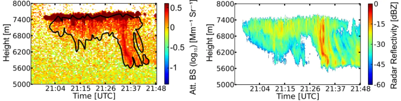
2.2 Case 2: colder mixed-phase cloud
Figure 1.Lidar and radar observations on 17 September 2011 (case 1). Left: lidar range-corrected 1064 nm signal (in logarithmic scale, arbitrary units a. u.); right: radar reflectivity. The dashed box denotes the region for which case 1 observations are shown in the following figures.
Figure 2.Cloudnet derived water contents for case 1. Left: liquid water content; right: ice water content (both in logarithmic scale).
same order of magnitude (see Fig. 5). Vertical wind speeds were in the same range as in the warmer case described above (Fig. 6).
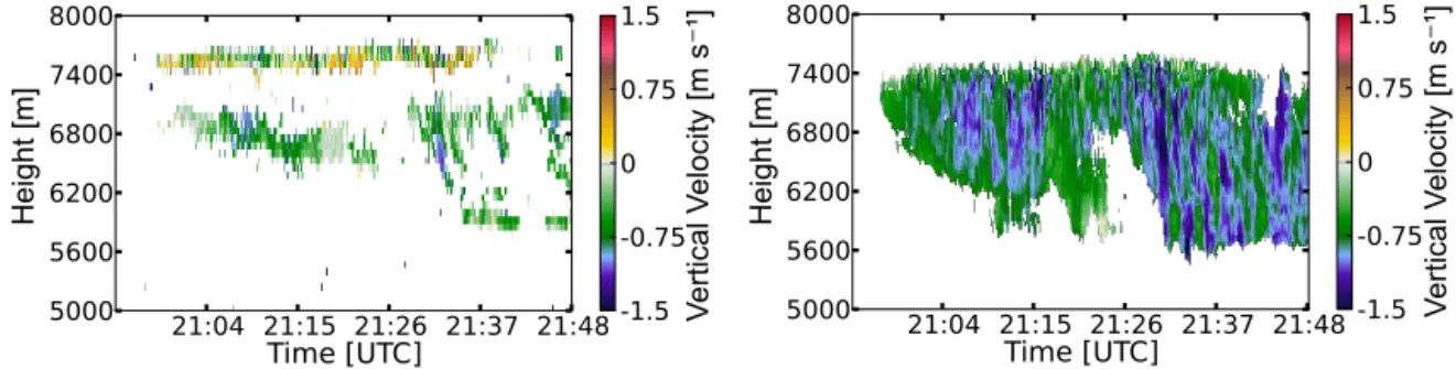
Accuracy of the IWC is±50 %. For the LWC calculated by the scaled adiabatic approach, the same order of mag-nitude applies. Vertical wind speeds are measured directly by evaluation from the recorded cloud radar and Doppler li-dar spectra. Errors are±0.15 m s−1for the cloud radar and ±0.05 m s−1for the Doppler lidar. These errors are mainly due to the pointing accuracy of the two systems.
3 Model description and initialization
For the model studies, an Asai–Kasahara (AK) type model is used (Asai and Kasahara, 1967). The model geometry is axisymmetric and consists of an inner and an outer cylinder with radii of 100 and 1000 m, respectively, resulting in a ra-dius ratio of 1:10, which is typical for this setup. However, the geometric configuration of the model is not intended to match the geometry of the clouds (and the cloud-free spaces between the clouds) but is rather meant to provide the pos-sibility of horizontal exchange between clouds and a cloud-free background.
The vertical resolution is constant with height and is cho-sen to be 1z=25 m to give a sufficient resolution of the cloud layer and to roughly match the vertical resolution of the observations. In contrast to a parcel model, the vertically
resolved model grid allows for a description of hydrometeor sedimentation. This is important especially for the fast grow-ing ice crystals to realistically describe their interaction with the vapor and liquid phase (Wegener–Bergeron–Findeisen process). A time step of 1 s was used for the dynamics as well as for the microphysics.
However, in contrast to other Asai–Kasahara model stud-ies, updrafts are not initialized by a heat and/or humidity pulse in certain layers for a given period of time. Instead, vertical velocity (updrafts and downdrafts) in the inner cylin-der is prescribed, which is more similar to a kinematic model like the Kinematic Driver model (KiD) (Shipway and Hill, 2012). In that way dynamics can be controlled to make sure that it is close to the observations.
Figure 3.Vertical velocity for case 1. Left: derived from lidar (valid for more numerous smaller droplets at cloud base); right: derived from radar observations (valid for large particles; virgae).
Figure 4.Lidar and radar observations on 2 August 2012 (case 2). Left: 532 nm attenuated backscatter coefficient; right: radar reflectivity.
base and sediments out soon). In addition, for case 1 ice par-ticle concentrations are low, which highly limits the probabil-ity of collisions. At the low temperatures of case 2 sticking efficiency is expected to be low. This assumption is corrobo-rated by the findings of Smith et al. (2009) stating that water vapor deposition (and sublimation), balanced by sedimenta-tion are more important than accresedimenta-tional growth.
3.1 Description of ice microphysics
In the following, the differences in the description of the mi-crophysics compared to Diehl et al. (2006) are described. 3.1.1 Immersion freezing
For this study, immersion freezing is assumed to be the only primary ice formation process. Since during the above-mentioned observations no in situ measurements of the INPs are available, the parameterization of DeMott et al. (2010) is used assuming that all INPs are active in the immersion freezing mode. The parameterization of DeMott et al. (2010) is based on an empirical relation of INPs and the number of aerosol particles with radii >250 nm (NAP, r>250 nm). To
cover case 1, the parameterization is extrapolated to −5◦C despite the fact that the underlying measurements were only taken at −9◦C and below. As base case NAP, r>250 nm=
105kg−1air is used as input data for the parameterization re-sulting in about 0.01 active INPs per liter for−6◦C (case 1) and about 0.5 INPs per liter for−25◦C (case 2) at standard
conditions. This corresponds to a relatively low number of larger aerosol particles but is well within the range observed by DeMott et al. (2010).
Figure 5.Cloudnet derived water contents for case 2. Left: liquid water content; right: ice water content (both in logarithmic scale).
Figure 6.Vertical velocity for case 2. Left: derived from lidar (valid for more numerous smaller droplets at cloud base); right: derived from radar observations (valid for large particles; virgae).
3.1.2 Ice particle shape
It is well known that ice particle shape highly influences wa-ter vapor deposition (described by changing the capacitance of the particle) as well as terminal fall velocity of the ice particle. Therefore, instead of the previously chosen spheri-cal ice particle shape, ice particles now can be prescribed as hexagonal columns or plates. The aspect ratio can be either constant for all size bins or be changed with size following the approach of Mitchell (1996). Typically, with increasing particle size, the deviation from an uniform aspect ratio in-creases. In our simulations, a constant uniform aspect ratio (ar=1) is used as base case. From Mitchell (1996) the size-varying aspect ratios for plates (ranging from 15 to 3000 µm with a single description) and columns (for size ranges of 30 to 100 µm, 100 to 300 µm, and above 300 µm in diameter) are calculated from the mass-dimension power laws and used for sensitivity studies.
The (relative) capacitance needed for the calculation of deposition growth of the ice crystals is modeled using the method of Westbrook et al. (2008) for the aspect ratios given above. Ice crystal terminal fall velocities are calculated ac-cording to Heymsfield and Westbrook (2010) using the same aspect ratios.
3.2 Model initialization 3.2.1 Thermodynamics
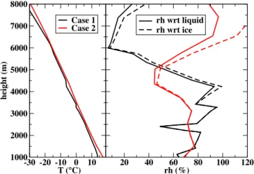
The Asai–Kasahara model has to be initialized with verti-cal profiles of temperature and dew point temperature either from reanalysis data (here GDAS) or radiosonde (RS) pro-files from nearby stations (here Meiningen, Thuringia). Fig-ure 7 shows profiles of temperatFig-ure and relative humidities with respect to liquid water and to ice, respectively, for both cases. For case 1, profiles from both methods show a simi-lar general behavior but the radiosonde profile of Meiningen measured at 00:00 UTC is used since it provides a finer ver-tical resolution than the GDAS reanalysis data (cp. Fig. 7). However, for case 2 the Meiningen RS profile misses the humidity layer at the level where the clouds were observed. This means that the profile is not representative for the given meteorological situation. Therefore, GDAS reanalysis data for Leipzig at 21:00 UTC were chosen. Finally, both profiles used show a sufficiently humid layer where the clouds were observed, so that the lifting of these layers leads to supersat-uration and subsequent cloud formation.
As mentioned above, vertical velocity (updrafts and down-drafts) in the inner cylinder is prescribed at cloud level rang-ing fromhbottohtop. The center of this interval is given by hmid=(htop+hbot)/2 and its half-depth byhdepth=(htop− hbot)/2.hbotranges from 3800 to 4100 m for case 1 and from
7000 to 7300 m for case 2. The respective values forhtopare
-30 -20 -10 0 10 T (°C) 1000
2000 3000 4000 5000 6000 7000 8000
height (m)
Case 1 Case 2
20 40 60 80 100 120
rh (%) rh wrt liquid rh wrt ice
Figure 7.Vertical profiles of temperature (left) and relative humid-ity (right) with respect to liquid water (full lines) and ice (dashed lines) based on a radiosonde observation (Meiningen) for case 1 (black) and from GDAS (grid point Leipzig) for case 2 (red).
given by
fh(h)=
h2depth−(h−hmid)2
h2depth forhbot≤h≤htop (1)
resulting in the time- and height-dependent function
w(h, t )=wmid(t )fh(h)forhbot≤h≤htop (2)
and w(h, t )=0 otherwise, defining wmid(t ) as the updraft
velocity at hmid. In order to match the observed wind field distributions rather closely,wmid(t )is chosen as a stochastic function
wmid(t )=wave+fscalδ(t )
3
|δ(t )|, (3)
where wave is the average (large-scale) updraft velocity at hmid varying between 0.1 m s−1 and 0.4 m s−1, fscal is the scaling factor determining the range of updraft velocities (chosen as 4 m s−1 to obtain a difference of minimum and maximum velocity of 2 m s−1), andδ(t )is a random number ranging from −0.5 to +0.5 obtained from a linear stochas-tic process provided by FORTRAN. After 30 s model time, a new δ(t )is created. Different realizations of the stochas-tic process are tested (see below). For example, wmid(t )
ranges from−0.7 m s−1to 1.3 m s−1ifw
ave=0.3 m s−1and fscal=4 m s−1as it is shown in the temporal evolution and
the histogram in Fig. 8.
Due to the height dependent vertical velocityw, a horizon-tal transport velocityuk (exchange between inner and outer cylinder) is induced in the Asai–Kasahara formulation for a given model layerk.
uk= −
wk+1
2
ρk+1
2−
wk−1
2
ρk−1
2
fr1zρk
(4)
Full indicesk indicate values at level centers whereas half indices (k+12,k+12) describe values at level interfaces.fr= 2/ri is a geometry parameter with the radiusri=100 m of the inner cylinder.
The prescribed velocity field leads to the following effects (all descriptions are related to the inner cylinder if not stated otherwise explicitly):
– In the updraft phase: in the upper part (betweenhmidand htop) of the updraft, mixing occurs from the inner to the
outer cylinder, whereas in the lower part (betweenhlow andhmid) horizontal transport is from the outer cylinder
into the inner one.
– For downdrafts it is the other way: this means that below
hmiddrops and ice particles are transported from the
in-ner cylinder to the outer one and are therefore removed from the inner cylinder.
– belowhlowor abovehtop, no horizontal exchange takes place.
The question arises to which extent this dynamical behavior reflects the real features of the observed clouds and whether this is critical for the topics aimed at in this study.
Prescribing vertical velocity in any way also means that a feedback of microphysics on dynamics due to phase changes (e.g., release of latent heat for condensing water vapor or freezing/melting processes) is not considered by the model. 3.2.2 Aerosol distribution
Since no in situ aerosol measurements are available, liter-ature data are used. The Raman lidar observations do not show any polluted layers for both cases; therefore, data from LACE98 (Petzold et al., 2002) are used which should be rep-resentative for the free troposphere over Leipzig. For case 1 values for the lower free troposphere (M6), for case 2 those from the upper free troposphere (M1), are used (see Petzold et al., 2002, Table 6).
4 Model results: dynamics
In a first step, the aim is to achieve a sufficient agreement concerning macroscopic cloud features, as well as (liquid phase) microphysics, as far as they were observed. The fol-lowing parameters describing model dynamics (updraft ve-locity) are varied to identify a “best case”, which in the sec-ond step can be used to perform sensitivity studies with re-spect to (ice) microphysics (see also Tables 1 and 2).
– hlow: ranging from 3800 to 4100 m for the warmer and
Figure 8.Vertical velocity field of the inner cylinder for case 1. Left: height dependence (red line) and temporal evolution of one realization of the stochastic vertical velocity field (black line) for wave=0.3 m s−1athmid. Right: histogram of velocity field. Vertical velocity for case 2 is identical but for heights between 7100 and 7700 m.
– wave: ranging from 0.1 to 0.4 m s−1. Higher average
up-draft also leads to higher LWC. Due to the lateral mix-ing processes the model setup requires a positive updraft velocity in average to form and maintain clouds. – δ: four different realizations of the stochastic process are
used. This influences the timing of the cloud occurrence as well as LWC and LWP but not systematically. All model results shown refer to the inner cylinder. 4.1 Case 1: warm mixed-phase cloud
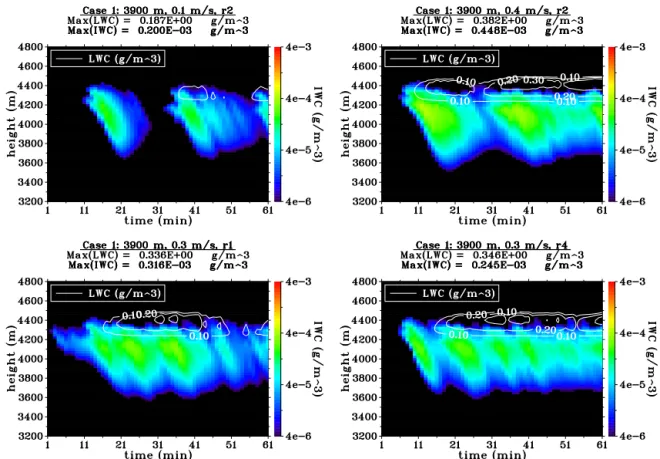
Figures 9 and 11 show time-height plots of the liquid- (con-tours, linear scale) and ice-water (colors, logarithmic scale) content for case 1 illustrating the cloud sensitivity with re-spect to variation of cloud base (hbot), average vertical
up-draft (wave), and the realization of the stochastic process.
Liq-uid clouds form in the updraft regions (cp. Fig. 8), whereas in the downdrafts the liquid phase vanishes at least partly. If active INPs are available ice formation can take place within the liquid part of the cloud. The INPs are partly already active near liquid cloud base, which means that they trigger freez-ing as soon as the droplets are formed. Less efficient INPs become active after further cooling above cloud base. Af-ter ice formation rapid depositional growth takes place and the ice particles almost immediately start to sediment. Due to the supersaturation with respect to ice even below liquid cloud base, ice particles still grow while sedimenting, reach-ing their maximum size before, finally, subsaturated regions are reached and sublimation sets in. Figures 10 and 12 show the time evolution of liquid (lower panel) and ice water path (upper panel) for the same parameters varied, reflecting the same temporal patterns. Table 1 summarizes the maximum values for LWC/IWC, LWP/IWP as well as cloud droplet and ice particle number concentration (CDN/IPN) for all dynam-ics sensitivity runs for case 1.
One can clearly observe, that a lowerhbot(Fig. 9) results
in a lower cloud base, larger vertical cloud extent as well
as more liquid water. The LWC maxima are within a fac-tor of 2 for varyinghbot. A similar trend is observed for the
ice phase (see also Fig. 10), but IWC maxima differ only by about 25 %. However, the values of the two maxima of the condensed phase after about 15–20 min and about 40 min model time are quite different. The first maximum is more pronounced for the ice phase whereas the second one is larger for the liquid phase. While the liquid phase is dominated by the updraft velocity (see Fig. 8) the ice phase additionally depends on INP supply. In the first ice formation event at 15 min, all INPs active at the current temperature actually form ice leading to an INP depletion. Due to the horizontal exchange with the outer cylinder the INP reservoir is refilled, but only to a certain extent when the second cloud event af-ter 40 min sets in. Due to the limited INP supply, the sec-ond ice maximum is weaker than the first one. The stochastic velocity fluctuations cause fluctuations in relative humidity, which are directly reflected by the liquid phase parameters, whereas the ice phase generally reacts much slower. Sensi-tivity of CDN and IPN with respect to change ofhbot does not seem to be systematic.
Table 1.Overview of the model results for the dynamic sensitivity runs for the warmer case 1 (maximum values of L/IWC: liquid/ice water content; L/IWP: liquid/ice water path; CDN: cloud drop number; IPN: ice particle number).
Run Parameter value LWC IWC LWP IWP CDN IPN
differing from base case g m−3 10−3g m−3 g m−2 10−3g m−2 cm−3 L−1
W_base – 0.355 0.379 41.33 62.27 46.89 0.0197
W_h38 hbot=3800 m 0.426 0.408 57.05 73.11 48.63 0.0235
W_h40 hbot=4000 m 0.289 0.357 28.58 58.12 61.48 0.0240
W_h41 hbot=4100 m 0.219 0.324 18.23 45.81 59.53 0.0208
W_w01 wave=0.1 m s−1 0.187 0.200 17.41 31.73 43.36 0.0138
W_w02 wave=0.2 m s−1 0.297 0.300 32.86 47.18 54.57 0.0175
W_w04 wave=0.4 m s−1 0.382 0.448 44.48 78.25 52.66 0.0219
W_r1 stoch. realiz. r1 0.336 0.316 40.32 54.85 64.26 0.0163
W_r3 stoch. realiz. r3 0.381 0.314 42.88 54.48 43.03 0.0167
W_r4 stoch. realiz. r4 0.346 0.245 40.91 46.93 47.42 0.0151
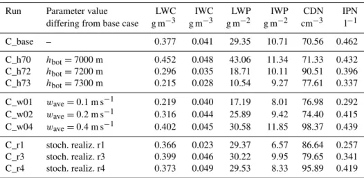
Table 2.Overview of the model results for the dynamic sensitivity runs for the colder case 2 (maximum values of L/IWC: liquid/ice water content; L/IWP: liquid/ice water path; CDN: cloud drop number; IPN: ice particle number).
Run Parameter value LWC IWC LWP IWP CDN IPN
differing from base case g m−3 g m−3 g m−2 g m−2 cm−3 l−1
C_base – 0.377 0.041 29.35 10.71 70.56 0.462
C_h70 hbot=7000 m 0.452 0.048 43.06 11.34 71.33 0.432 C_h72 hbot=7200 m 0.296 0.035 18.71 10.11 90.51 0.396
C_h73 hbot=7300 m 0.215 0.028 10.54 9.27 77.61 0.337
C_w01 wave=0.1 m s−1 0.219 0.040 17.19 8.01 76.98 0.292 C_w02 wave=0.2 m s−1 0.316 0.044 25.89 9.42 74.40 0.415 C_w04 wave=0.4 m s−1 0.402 0.045 30.58 11.85 98.37 0.439
C_r1 stoch. realiz. r1 0.366 0.023 29.37 6.57 86.64 0.257 C_r3 stoch. realiz. r3 0.399 0.046 30.22 9.95 79.65 0.341 C_r4 stoch. realiz. r4 0.373 0.049 29.53 8.33 95.89 0.419
Figures 11 (lower panel) and 12 (right) show that differ-ent realizations of the stochastic process (as explained above in Sect. 3.2.1) lead to different temporal cloud evolutions. However, differences in maximum LWP and LWC are much smaller than those discussed above. Variations in maximum IWP and IWC, as well as CDN and IPN, are in the range of about 30 %. This is also true for average LWP ranging from 18 g m−2for W_r1 to 26 g m−2for W_r3. However, despite the different maxima and temporal evolutions of IWP, aver-age IWP is almost identical for the different stochastic real-izations (0.023 g m−2). This shows that changing the stochas-tic realization influences cloud evolution in detail (timing) but does not change the overall picture.
With maximum values between 17 and 57 g m−2, the modeled liquid water path is in the same range as the ob-served values (20–50 g m−2), especially for the “wetter” runs (smallerhbot, largerwave). Average LWP typically is about half (40–60 %) of the maximum value for most of the runs,
which also fits well into the observations. Ice forms within the liquid layer and sediments to about 3800 m for most runs, which is less than for the observations. The (maximum) mod-eled ice mixing ratio is in the same order of magnitude as the observed one (about 10−7kg m−3). The same holds for
the ice water path with values of about 0.01 g m−2for both,
model and observation. For the other values, no observational data are available for comparison.
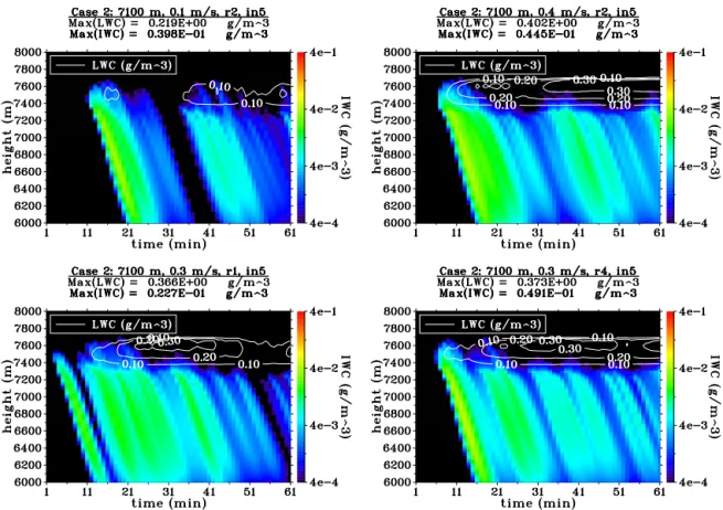
4.2 Case 2: colder mixed-phase cloud
Figure 9.LWC (contours) and IWC (colors, logarithmic scale) for case 1. Comparison of different values forhbot(upper left: W_base, hbot=3900 m; upper right: W_h38,hbot=3800 m; lower left: W_h40,hbot=4000 m; lower right: W_h41,hbot=4100 m.)
0 10 20 30 40 50 60
time (min) 0
10 20 30 40 50 60
L
WP
(g/sqm)
W_base W_h38 W_h40 W_h41 0
0,02 0,04 0,06 0,08
IWP
(g/sqm)
Figure 10.Liquid (lower panel) and ice water paths (upper panel) for case 1. Comparison of the different values forhbot.
down to more than 1500 m below liquid cloud base, which is in concordance with the observations. The principal be-havior with respect to the sensitivity parameters is similar to case 1: the liquid phase is enhanced by either decreasinghbot
or increasing wave, showing the “saturation” effect slightly
more pronounced as in case 1. Different stochastic
realiza-tions only weakly influence the maximum and average val-ues of the liquid phase but change the timing of occurrence. Generally, the variability of the ice phase is weaker than in case 1. The different stochastic realizations show the high-est variability in IWC and IWP. Different variations ofhbot
show almost identical IWPs, whereas changingwaveat least slightly influences maximum IWC and IWP, which again can be attributed to the ice particle accumulation in the updraft. Liquid water path is smaller than in case 1 and reaches max-imum values between 10 and 43 g m−2, which well covers
the observed maximum value of about 20 g m−2. Cloudnet observations show an IWC of 10−7–10−5kg m−3, which is an increase by a factor of 10–100 compared to case 1. Sim-ilar values are obtained by the model results underlining the strong temperature dependency of the ice nucleation process.
5 Sensitivity studies
Figure 11.LWC (contours) and IWC (colors, logarithmic scale) for case 1. Comparison of different average updraft velocitieswave(upper panel: left: W_w01,wave=0.1 m s−1; right: W_w04,wave=0.4 m s−1) and different stochastic realizations (lower: left: W_r1, r1; right: W_r4, r4).
0 10 20 30 40 50 60
time (min) 0
10 20 30 40 50 60
L
WP
(g/sqm)
W_base W_w01 W_w02 W_w04 0
0,02 0,04 0,06 0,08
IWP
(g/sqm)
0 10 20 30 40 50 60
time (min) 0
10 20 30 40 50 60
L
WP
(g/sqm)
W_base W_r1 W_r3 W_r4 0
0,02 0,04 0,06 0,08
IWP
(g/sqm)
Figure 12.Liquid (lower panels) and ice water paths (upper panels) for case 1. Comparison of the different values forwave(left) and the different stochastic realizations (right).
question of which microphysical parameters are expected to have a large influence on mixed phase microphysics and are rather uncertain to be estimated. This leads to a (temperature-dependent) INP number (NINP) that directly influences the
ice particle number but mostly is poorly known. To be consis-tent with the freezing parameterization of the model,NINPis varied by changingNAP, r>250 nm, which additionally is
eas-ier to observe in most cases. A second parameter is the shape
Figure 13.LWC (contours) and IWC (colors, logarithmic scale) for case 2. Comparison of different values forhbot(upper left: C_base, hbot=7100 m; upper right: C_h70,hbot=7000 m; lower left: C_h72,hbot=7200 m; lower right: C_h73,hbot=7300 m).
0 10 20 30 40 50 60
time (min) 0
10 20 30 40 50
L
WP
(g/sqm)
C_base C_h70 C_h72 C_h73 0
5 10 15 20
IWP
(g/sqm)
Figure 14.Liquid (lower panel) and ice water paths (upper panel) for case 2. Comparison of the different values forhbot.
5.1 INP number
Changing NAP, r>250 nm leads to a temperature-dependent
change of INP number, which is relatively small for warmer conditions. However, the effect increases with decreasing temperature. This is illustrated by the following numbers.
The parameterization of DeMott et al. (2010) gives about 0.009 active INPs per liter at standard conditions (NINP)
whenNAP, r>250 nm=105kg−1atT = −5◦C. A tenfold
in-crease to NAP, r>250 nm=106kg−1results in about 0.012
ac-tive INPs per liter, which is a rise of only about 35 %. For
T = −7◦C, INP number rises by about 65 % for a tenfold increase of NAP, r>250 nm. This shows that for those rather
high temperatures considered for case 1, a massive change in
NAP, r>250 nm leads to relatively small changes inNINP and
only a small effect on the ice phase can be expected. This is confirmed by Fig. 17 (left) showing liquid and ice water contents for W_in6. IWC is enhanced by less than 60 % for W_in6 and by about 160 % for W_in7, which is consistent for the given temperature range (see Table 3). Similar val-ues are obtained for the change in IPN. This directly leads to the conclusion that the individual ice particles grow indepen-dently from each other. Their individual growth history is (in contrast to drop growth) only influenced by thermodynamics as long as their number is low enough, which seems to be the case here.
Figure 15.LWC (contours) and IWC (colors, logarithmic scale) for case 2. Comparison of different average updraft velocitieswave(upper left: C_w01,wave=0.1 m s−1, right: C_w04,wave=0.4 m s−1) and the different stochastic realizations (lower left: C_r1, r1, right: C_r4, r4).
Table 3.Overview of the model results for the microphysical sensitivity runs for the warmer case 1 (maximum values of L/IWC: liquid/ice water content, L/IWP: liquid/ice water path, CDN: cloud drop number, IPN: ice particle number).
Run Parameter value LWC IWC LWP IWP CDN IPN
differing from base case g m−3 10−3g m−3 g m−2 g m−2 cm−3 l−1
W_in6 NAP, r>250 nm=106kg−1 0.354 0.619 41.31 0.10 46.69 0.0296 W_in7 NAP, r>250 nm=107kg−1 0.354 1.000 41.24 0.17 41.61 0.0450
W_col ice shape: columns 0.353 1.830 41.20 0.27 42.90 0.0257
W_pla ice shape: plates 0.353 2.850 41.13 0.45 43.41 0.0267
number and mass, the shape of the ice particle size distri-bution (colors) is not changed. The smallest ice particles can be observed at three discrete height (and temperature) levels caused by the temperature resolved parameterization of the potential INPs described in Sect. 3.1.1. In reality this part of the spectrum showing rather freshly nucleated and fast grow-ing ice particles should be continuous over the height range from about 4100 to 4400 m. Nevertheless, the total number of ice particles formed is described correctly.
One can conclude that increasing INP number therefore increases ice particle number as well as ice mass propor-tionally. Generally, the ice mass remains small and the liquid phase is not affected by the ice mass increase. Those results
are supported by Fig. 19 (left) showing an unchanged LWP and a proportionally growing IWP for increased INP num-bers.
For the colder case 2 the parameters are varied in the same way. However, one big difference is that a tenfold increase of
NAP, r>250 nmatT = −25◦C results in a much larger change
en-0 10 20 30 40 50 60 time (min)
0 10 20 30 40 50
L
WP
(g/sqm)
C_base C_r1 C_r3 C_r4 0
5 10 15 20
IWP
(g/sqm)
0 10 20 30 40 50 60
time (min) 0
10 20 30 40 50
L
WP
(g/sqm)
C_base C_w01 C_w02 C_w04 0
5 10 15 20
IWP
(g/sqm)
Figure 16.Liquid (lower panels) and ice water paths (upper panels) for case 2. Comparison of the different values forwave(left) and the different stochastic realizations (right).
Figure 17.LWC (colors) and IWC (contours, logarithmic scale) for case 1 (W_in6, left) and case 2 (C_in6, right). Enhancing IN by increasing
NAP, r>250 nmby a factor of 10.
hanced by a factor of 3–4 for C_in6 and about 10 for C_in7 whereas IPN increases by a factor of 12. This can also be seen in the IWP (Fig. 19, right, red lines) showing a limited increase for C_in7, especially for the first maximum after 17 min. This means that the results for C_in6 are still con-sistent with an independent growth of the individual ice par-ticles (as described above) despite the relatively high ice oc-currence.
This is verified by the size distributions in Fig. 18 (lower panel). As in case 1 the ice particle size distributions only differ by the number/mass, but not by shape. Additionally, the decrease in the liquid phase is reflected also in the drop spectrum showing a more shallow liquid part of cloud as well as droplet distribution shifted to smaller sizes.
However, for C_in7 the ice particles compete for water vapor, which becomes clear from (i) the depletion of liquid water (resulting in a lower supersaturation with respect to ice) and (ii) the ice mass enhancement factor being below the value expected from the ice nucleation parameterization and below that of IPN. This means that despite the higher number of INPs and, therefore, ice particles, the amount of
ice is limited by the thermodynamic conditions that result in the production of more but smaller ice particles, similar to the Twomey effect for drop activation.
As mentioned earlier, ice particle growth is not only re-stricted to the liquid part of the cloud but also occurs in the layer below liquid cloud base, which is still supersaturated with respect to ice. This leads to a decrease in relative hu-midity in this part of the cloud, which in turn weakens or suppresses droplet formation by shifting liquid cloud base to higher altitudes. The lower LWC for the runs with higher IWC therefore cannot only be attributed to the WBF pro-cesses but also to this indirect effect.
5.2 Ice particle shape
Figure 18.LWC (contours) and IWC per bin (colors, both logarithmic scale) for case 1 (upper panel) and case 2 (lower panel) for the respective base case (left) and the case with enhanced IN number (right; in6) after 16 and 17 minutes model time, respectively, corresponding to the IWP maximum of the base case runs.
Table 4.Overview of the model results for the microphysical sensitivity runs for the colder case 2 (maximum values of L/IWC: liquid/ice water content; L/IWP: liquid/ice water path; CDN: cloud drop number; IPN: ice particle number).
Run Parameter value LWC IWC LWP IWP CDN IPN
differing from base case g m−3 g m−3 g m−2 g m−2 cm−3 l−1
C_in6 NAP, r>250 nm=106kg−1 0.224 0.140 13.09 34.75 80.29 1.380 C_in7 NAP, r>250 nm=107kg−1 0.036 0.446 2.58 57.98 46.67 5.208
C_col ice shape: columns 0.237 0.223 14.33 46.78 78.40 0.462
C_col_in4 ice shape: columns,NAP, r>250 nm=104kg−1 0.378 0.076 30.01 14.93 74.75 0.139
C_pla ice shape: plates 0.182 0.294 9.94 57.11 39.41 0.472
C_pla_in4 ice shape: plates,NAP, r>250 nm=104kg−1 0.362 0.102 27.80 19.21 74.44 0.129
particle shape from quasi-spherical (ar=1) to columns or plates with size-dependent axis ratios deviating from unity results in an increase of water vapor deposition on the in-dividual ice particles leading to enhanced ice water content due to larger individual particles when ice particle numbers remain unchanged. This is due to (i) enhanced relative ca-pacitance resulting in faster water vapor deposition and (ii) lower terminal velocities of the ice particles leading to longer residence times in vicinity of conditions with supersaturation with respect to ice.
0 10 20 30 40 50 60 time (min) 0 10 20 30 40 50 L WP (g/sqm) C_base C_in6 C_in7 C_col C_pla C_col_in4 C_pla_in4 0 10 20 30 40 50 60 IWP (g/sqm)
0 10 20 30 40 50 60
time (min) 0 10 20 30 40 50 60 L WP (g/sqm) W_base W_in6 W_in7 W_col W_pla 0 0,1 0,2 0,3 0,4 0,5 IWP (g/sqm)
Figure 19.Liquid (lower panel) and ice water paths (upper panel) for case 1 (left) and case 2 (right). Comparison of the sensitivities with respect to IN number and ice particle shape.
upper left panel W_col is shown after 16 min correspond-ing to Fig. 18. Compared to W_base, larger ice particles are produced leading to more ice mass (equivalent radius up to 300 µm compared to 189–238 µm for the base case). Additionally, due to the lower fall speed of the columns (1.03 m s−1 vs. 1.75–2.24 m s−1), the maximum of the ice
is at about 4200 m compared to 4100 m for the base case. On the upper right panel, size distributions after 21 min are shown corresponding to the IWP maximum of W_col. Ice particles have grown larger (equivalent radius up to 378 µm, length of the columns increases from about 3 to 4.5 mm) and sedimentation has developed further with increasing terminal velocity (1.13 m s−1). Similar results are obtained for plates (W_pla) with terminal velocities of 0.89–1.21 m s−1, equiv-alent radii of 300–476 µm, and maximum dimension of 1.8– 3.2 mm.
The lower terminal velocity of columns and plates despite their larger size is leading to the stronger tilting of the virgae. Additionally, the IPN is enhanced by about 30 % although ice nucleation is identical to W_base. This can be attributed to the lower fall velocities, too, leading to an accumulation of ice particles. The differences between W_col and W_pla are caused by both, the higher relative capacitances of and lower terminal fall velocities of plates compared to columns (at least when their axis ratios are chosen following (Mitchell, 1996)).
For case 2 (C_col and C_pla), the liquid water reduction due to the Bergeron–Findeisen process is similar to C_in6 (see Fig. 20, right, and Table 4). In contrast to the respec-tive case 1 runs, less ice is produced than for C_in7. The tilting of the virgae is not as strong as in W_col, which is due to the larger ice particle sizes leading to higher termi-nal fall velocities (1.43–1.60 m s−1). Additionally, the lower air density leads to an increase of terminal velocity of more than 10 % independently from shape. Figure 21 (lower panel) shows the size distributions for C_col at different times. Due to the longer growth time larger individual ice particles than
in case 1 are produced (equivalent radius up to 600 µm com-pared to 300 µm for the base case).
To decide whether independent ice particle growth or com-petition occurs, further runs with less INPs (C_col_in4 and C_pla_in4) are discussed (see Fig. 19, right). IWC and IWP of these runs (in4) are about one-third of the values of the respective runs with more INPs (in5). For ice particle num-ber, a factor of slightly more than 3 occurs, which means that a weak competition for water vapor occurs for C_col and C_pla resulting in slightly smaller individual ice parti-cles compared to C_col_in4 and C_pla_in4.
6 Conclusions
The model system AK–SPECS was applied to simulate dy-namical and microphysical processes within altocumulus clouds. Sensitivity studies on relative contributions on cloud evolution as well as comparisons to observations were made. Variation of the dynamic parameters as it was done in Sect. 4 leads to systematic differences mainly in the liquid phase (LWC, LWP), which can easily be explained. More liq-uid water is produced when either cloud base is lowered (cor-responding to a larger vertical cloud extent) or vertical wind velocity is increased. However, the effects of the dynamics on the ice phase are surprisingly small, at least smaller than those on the liquid phase. Increasing vertical velocity leads to an accumulation of the smaller ice particles in the enhanced updraft.
On the other hand, much larger differences in terms of IWC and IWP were found when microphysical parameters like INP number or ice particle shape were varied under iden-tical dynamic conditions. This is valid for both cases stud-ied. However, at least for the ice nucleation parameterization used, sensitivity of INP number strongly increased with de-creasing temperature.
dif-Figure 20.LWC (contours) and IWC (colors, logarithmic scale). Results for changing ice particle shape to hexagonal columns for case 1 (W_col, left) and case 2 (C_col, right).
Figure 21.LWC (contours) and ice water mass per bin (colors, both logarithmic scale) for case 1 (upper panel) and case 2 (lower panel) assuming columns as ice particle shape at IWP maximum of the respective base case (left) and at IWP of the run (right).
fers considerably or ice particle shape is different (which should not be the case for relatively similar thermodynami-cal conditions). After Fukuta and Takahashi (1999) for case 1 with temperatures of about−6◦C, column-like ice particles withar=0.1 could be expected (corresponding to W_col), whereas for case 2 (T <−24◦C) hexagonal particles with
ar=1 are most likely (e.g., C_base). Those ice shapes were observed in laboratory studies at water saturation, which was
present, which typically is the case for cold conditions with a sufficient amount of INPs and fast growing ice particle shapes (most effective for large deviations from spherical shapes).
Acknowledgements. This study was supported by the Deutsche
Forschungsgemeinschaft (DFG) under grant AN 258/15. We also acknowledge funding from the EU FP7-ENV-2013 programme “impact of Biogenic vs. Anthropogenic emissions on Clouds and Climate: towards a Holistic UnderStanding” (BACCHUS), project no. 603445.
Edited by: T. Garrett
References
Althausen, D., Engelmann, R., Baars, H., Heese, B., Ansmann, A., Müller, D., and Komppula, M.: Portable Raman Lidar Pol-lyXT for Automated Profiling of Aerosol Backscatter, Extinc-tion, and DepolarizaExtinc-tion, J. Atmos. Oceanic Technol., 26, 2366– 2378, 2009.
Asai, T. and Kasahara, A.: A theoretical study of compensating downward motions associated with cumulus clouds, JOURNAL OF THE ATMOSPHERIC SCIENCES, 24, 487–496, 1967. Bauer-Pfundstein, M. R. and Görsdorf, U.: Target Separation and
Classification Using Cloud Radar Doppler-Spectra, in: Proceed-ings of the 33rd Conference on Radar Meteorology, 2007. Bergeron, T.: On the physics of clouds and precipitation, in:
Pro-ces verbaux de l’association de Météorologie, pp. 156–178, In-ternational Union of Geodesy and Geophysics, Lisboa, Portugal, 1935.
Bühl, J., Ansmann, A., Seifert, P., Baars, H., and Engelmann, R.: Toward a quantitative characterization of heterogeneous ice formation with lidar/radar: Comparison of CALIPSO/CloudSat with ground-based observations, Geophys. Res. Lett., 40, 4404– 4408, 2013.
Bühl, J., Engelmann, R., and Ansmann, A.: Removing the Laser-Chirp Influence from Coherent Doppler Lidar Datasets by Two-Dimensional Deconvolution, J. Atmos. Oceanic Technol., 29, 1042–1051, 2012.
Carey, L. D., Niu, J., Yang, P., Kankiewicz, J. A., Larson, V. E., and Vonder Haar, T. H.: The Vertical Profile of Liquid and Ice Water Content in Midlatitude Mixed-Phase Altocumulus Clouds, J. Appl. Meteorol. Climate, 47, 2487–2495, 2008.
Dearden, C., Connolly, P. J., Choularton, T., Field, P. R., and Heymsfield, A. J.: Factors influencing ice formation and growth in simulations of a mixed-phase wave cloud, J. Adv. Model. Earth Syst., 4, M10001, doi:10.1029/2012MS000163, 2012. DeMott, P. J., Prenni, A. J., Liu, X., Kreidenweis, S. M., Petters,
M. D., Twohy, C. H., Richardson, M. S., Eidhammer, T., and Rogers, D. C.: Predicting global atmospheric ice nuclei distribu-tions and their impacts on climate, PROCEEDINGS OF THE NATIONAL ACADEMY OF SCIENCES OF THE UNITED STATES OF AMERICA, 107, 11217–11222, 2010.
Diehl, K., Simmel, M., and Wurzler, S.: Numerical sensitivity stud-ies on the impact of aerosol propertstud-ies and drop freezing modes
on the glaciation, microphysics, and dynamics of clouds, J. Geo-phys. Res.-Atmos., 111, D07202, doi:10.1029/2005JD005884, 2006.
Eidhammer, T., DeMott, P. J., Prenni, A. J., Petters, M. D., Twohy, C. H., Rogers, D. C., Stith, J., Heymsfield, A., Wang, Z., Pratt, K. A., Prather, K. A., Murphy, S. M., Seinfeld, J. H., Subrama-nian, R., and Kreidenweis, S. M.: Ice Initiation by Aerosol Par-ticles: Measured and Predicted Ice Nuclei Concentrations ver-sus Measured Ice Crystal Concentrations in an Orographic Wave Cloud, J. Atmos. Sci., 67, 2417–2436, 2010.
Field, P. R., Heymsfield, A. J., Shipway, B. J., DeMott, P. J., Pratt, K. A., Rogers, D. C., Stith, J., and Prather, K. A.: Ice in Clouds Experiment-Layer Clouds, Part II: Testing Characteris-tics of Heterogeneous Ice Formation in Lee Wave Clouds, J. At-mos. Sci., 69, 1066–1079, 2012.
Findeisen, W.: Kolloid-meteorologische Vorgänge bei Nieder-schlagsbildung, Meteorolog. Z., 55, 121–133, 1938.
Fleishauer, R. P., Larson, V. E., and Vonder Haar, T. H.: Observed Microphysical Structure of Midlevel, Mixed-Phase Clouds, J. At-mos. Sci., 59, 1779–1804, 2002.
Fridlind, A. M., Ackerman, A. S., McFarquhar, G., Zhang, G., Poel-lot, M. R., DeMott, P. J., Prenni, A. J., and Heymsfield, A. J.: Ice properties of single-layer stratocumulus during the Mixed-Phase Arctic Cloud Experiment: 2. Model results, J. Geophys. Res.-Atmos., 112, D24202, doi:10.1029/2007JD008646, 2007. Fukuta, N. and Takahashi, T.: The Growth of Atmospheric Ice
Crys-tals: A Summary of Findings in Vertical Supercooled Cloud Tun-nel Studies, J. Atmos. Sci., 56, 1963–1979, 1999.
Hartmann, S., Augustin, S., Clauss, T., Wex, H., Santl-Temkiv, T., Voigtlander, J., Niedermeier, D., and Stratmann, F.: Immer-sion freezing of ice nucleation active protein complexes, Atmos. Chem. Phys., 13, 5751–5766,
doi10.5194/acp-13-5751-2013, 2013.
Heymsfield, A. J. and Westbrook, C. D.: Advances in the Estimation of Ice Particle Fall Speeds Using Laboratory and Field Measure-ments, J. Atmos. Sci., 67, 2469–2482, 2010.
Hogan, R. J., Mittermaier, M. P., and Illingworth, A. J.: The Re-trieval of Ice Water Content from Radar Reflectivity Factor and Temperature and Its Use in Evaluating a Mesoscale Model, J. Appl. Meteor. Climatol., 45, 301–317, 2006.
Illingworth, A. J., Hogan, R. J., O’Connor, E. J., Bouniol, D., De-lanoë, J., Pelon, J., Protat, A., Brooks, M. E., Gaussiat, N., Wil-son, D. R., Donovan, D. P., Baltink, H. K., van Zadelhoff, G.-J., Eastment, J. D., Goddard, J. W. F., Wrench, C. L., Haeffelin, M., Krasnov, O. A., Russchenberg, H. W. J., Piriou, J.-M., Vinit, F., Seifert, A., Tompkins, A. M., and Willén, U.: Cloudnet, Bull. Amer. Meteor. Soc., 88, 883–898, 2006.
Kanitz, T., Seifert, P., Ansmann, A., Engelmann, R., Althausen, D., Casiccia, C., and Rohwer, E. G.: Contrasting the impact of aerosols at northern and southern midlatitudes on heterogeneous ice formation, Geophysical Res. Letters, 38, L17802,
doi10.1029/2011GL048532, 2011.
Korolev, A. and Field, P. R.: The Effect of Dynamics on Mixed-Phase Clouds: Theoretical Considerations, J. Atmos. Sci., 65, 66–86, 2008.
Mitchell, D.: Use of mass- and area-dimensional power laws for determining precipitation particle terminal velocities, J. Atmos. Sci., 53, 1710–1723, 1996.
Murray, B. J., O’Sullivan, D., Atkinson, J. D., and Webb, M. E.: Ice nucleation by particles immersed in supercooled cloud droplets, Chem. Soc. Rev., 41, 6519–6554, 2012.
O’Sullivan, D., Murray, B. J., Malkin, T. L., Whale, T. F., Umo, N. S., Atkinson, J. D., Price, H. C., Baustian, K. J., Browse, J., and Webb, M. E.: Ice nucleation by fertile soil dusts: relative importance of mineral and biogenic components, Atmos. Chem. Phys., 14, 1853–1867, 2014.
Petzold, A., Fiebig, M., Flentje, H., Keil, A., Leiterer, U., Schroder, F., Stifter, A., Wendisch, M., and Wendling, P.: Vertical variabil-ity of aerosol properties observed at a continental site during the Lindenberg Aerosol Characterization Experiment (LACE 98), J. Geophys. Res.-Atmos., 107, 8128, doi:10.1029/2001JD001043, 2002.
Phillips, V. T. J., DeMott, P. J., and Andronache, C.: An empiri-cal parameterization of heterogeneous ice nucleation for multi-ple chemical species of aerosol, J. Atmos. Sci., 65, 2757–2783, 2008.
Pospichal, B., Kilian, P., and Seifert, P.: Performance of cloud liquid water retrievals from ground-based remote sensing observations over Leipzig, in: Proceedings of the 9th International Symposium on Tropospheric Profiling (ISTP), 2012.
Shipway, B. J. and Hill, A. A.: Diagnosis of systematic differences between multiple parametrizations of warm rain microphysics using a kinematic framework, Q. J. R. Meteorol. Soc., 138, 2196– 2211, 2012.
Simmel, M. and Wurzler, S.: Condensation and activation in sec-tional cloud microphysical models, Atmos. Res., 80, 218–236, 2006.
Smith, A. J., Larson, V. E., Niu, J., Kankiewicz, J. A., and Carey, L. D.: Processes that generate and deplete liquid water and snow in thin midlevel mixed-phase clouds, J. Geophys. Res., 114, D12203, 2009.
Sun, J., Ariya, P. A., Leighton, H. G., and Yau, M. K.: Modeling Study of Ice Formation in Warm-Based Precipitating Shallow Cumulus Clouds, J. Atmos. Sci., 69, 3315–3335, 2012. Warren, S. G., Hahn, C. J., London, J., Chervin, R. M., and Jenne,
R.: Global distribution of total cloud cover and cloud type amount over land, Tech. Rep. Tech. Note TN-317 STR, NCAR, 1998a.
Warren, S. G., Hahn, C. J., London, J., Chervin, R. M., and Jenne, R.: Global distribution of total cloud cover and cloud type amount over the ocean, Tech. Rep. Tech. Note TN-317 STR, NCAR, 1998b.
Wegener, A.: Thermodynamik der Atmosphäre, J. A. Barth Verlag, 1911.