Estimates of mercury flux into the United States from non-local and global sources: results from a 3-D CTM simulation

(1)

ACPD

8, 19861–19890, 2008

Mercury fluxes into the US from non-local

and global sources

B. A. Drewniak et al.

Title Page

Abstract Introduction

Conclusions References

Tables Figures

◭ ◮

Back Close

Full Screen / Esc

Printer-friendly Version

Interactive Discussion Atmos. Chem. Phys. Discuss., 8, 19861–19890, 2008

www.atmos-chem-phys-discuss.net/8/19861/2008/ © Author(s) 2008. This work is distributed under the Creative Commons Attribution 3.0 License.

Atmospheric Chemistry and Physics Discussions

This discussion paper is/has been under review for the journalAtmospheric Chemistry and Physics (ACP). Please refer to the corresponding final paper inACPif available.

Estimates of mercury flux into the United

States from non-local and global sources:

results from a 3-D CTM simulation

B. A. Drewniak1, V. R. Kotamarthi1, D. Streets2, M. Kim3, and K. Crist3

1

Environmental Science Division, Argonne National Laboratory, Argonne, IL, USA 2

Decision and Information Sciences Division, Argonne National Laboratory, Argonne, IL, USA 3

Department of Chemical Engineering, Ohio University, Athens, OH, USA

Received: 28 August 2008 – Accepted: 7 October 2008 – Published: 27 November 2008

Correspondence to: V. R. Kotamarthi (vrkotamarthi@anl.gov)

(2)

ACPD

8, 19861–19890, 2008

Title Page

Tables Figures

◭ ◮

Back Close

Full Screen / Esc

Interactive Discussion

Abstract

The sensitivity of Hg concentration and deposition in the United States to emissions in China was investigated by using a global chemical transport model: Model for Ozone and Related Chemical Tracers (MOZART). Two forms of gaseous Hg were included in the model: elemental Hg (HG(0) and oxidized or reactive Hg (HGO). We simulated 5

three different emission scenarios to evaluate the model’s sensitivity. One scenario included no emissions from China, while the others were based on different estimates of Hg emissions in China. The results indicated, in general, that when Hg emissions were included, HG(0) concentrations increased both locally and globally. Increases in Hg concentrations in the United States were greatest during spring and summer, by as 10

much as 7%. Ratios of calculated concentrations of Hg and CO near the source region in eastern Asia agreed well with ratios based on measurements. Increases similar to those observed for HG(0) were also calculated for deposition of HGO. Calculated increases in wet and dry deposition in the United States were 5–7% and 5–9%, re-spectively. The results indicate that long-range transcontinental transport of Hg has a 15

non-negligible impact on Hg deposition levels in the United States.

1 Introduction

Mercury in the environment poses a risk to human health (NRC, 2000). Environmen-tal Hg levels around the world have increased considerably in recent years, and even regions with no significant emissions, such as the Arctic, are a_ffected by the transcon-20

tinental transport of Hg. Modeling studies and measurements have confirmed the ability of elemental Hg (HG(0) to be transported over long distances (Seigneur et al., 2001; Travnikov and Ryaboshapko, 2002; Banic et al., 2003; Dastoor and Larocque, 2004). This finding has generated concern in the United States that substantial quan-tities of long-range-transported atmospheric Hg might interfere with the ability of do-25

(3)

ACPD

8, 19861–19890, 2008

Title Page

Tables Figures

◭ ◮

Back Close

Full Screen / Esc

Interactive Discussion Seigneur et al., 2004). Mercury emissions from anthropogenic sources in rapidly

grow-ing economies in Asia and their impact on global Hg concentrations are of concern (Jaffe et al., 2005). Seigneur et al. (2004) estimated that anthropogenic emission of Hg in Asia contributed 21% of the total Hg deposition in the contiguous United States in 1998.

5

In this study, we coupled new emission inventories for China with a global chemical transport model (CTM) to perform a fresh assessment of the relative contributions of local and distant sources to Hg deposition in the United States. An existing global-scale three-dimensional (3-D) CTM, the Model for Ozone and Related Chemical Trac-ers (MOZART), was modified to include gas-phase Hg chemistry. Simulations were 10

performed by using the National Center for Environmental Prediction (NCEP) assim-ilated dynamic fields for the year 2004. Several calculations were performed to test the sensitivity of US atmospheric Hg concentrations and deposition fluxes to a set of emission estimates from China, as follows:

– The first calculation was performed by using the global-scale emissions developed 15

by Pacyna et al. (2006).

– A second estimate of emissions from China, developed by Streets et al. (2005), was substituted for the Pacyna et al. (2006) estimate in the second calculation.

– In a third calculation, we assign net zero emissions of Hg from China, while re-taining the Pacyna et al. (2006) estimate for the rest of the world.

20

We present results from these simulations, particularly the expected contribution of sources in Asia to the US atmosphere. Our primary aim was to investigate the impact of this range of emissions from China on the United States, rather than focusing on uncertainties in the chemical mechanism leading to the formation of oxidized or reactive Hg (HGO) from HG(0).

(4)

ACPD

8, 19861–19890, 2008

Title Page

Tables Figures

◭ ◮

Back Close

Full Screen / Esc

Interactive Discussion

2 Methods

2.1 Model framework

We used MOZART as described in Horowitz et al. (2003) and Wei et al. (2002), mod-ified to include Hg chemistry. The grid resolution was based on meteorology data at 2.8 degrees latitude×2.8 degrees longitude, with 28 vertical levels extending from the 5

surface to 2.7 mb. This model accounts for surface emissions (including N₂O, CH₄, CO, NO_x, NMHC, CH₂O, isoprene, acetone, etc.), chemical and photochemical reactions, advection, convection, and wet and dry deposition. The emission fluxes in MOZART for anthropogenic species were based on the Emission Database for Global Atmospheric Research (EDGAR) (Olivier et al., 1996). The version of MOZART used here provides 10

spatial and temporal distributions for 52 chemical tracers, with a chemistry scheme similar to the one described by Brasseur et al. (1998), which incorporates 107 gas-phase, 5 heterogeneous, and 29 photochemical reactions. Empirical first-order het-erogeneous reactions involving N₂O₅and NO₃on sulfate aerosols are implemented in the model (see M ¨uller and Brasseur (1995) for details). Advection of the trace gases 15

was simulated by using the flux-form semi-Lagrangian (FFSL) formulation of Lin and Rood (1996), which replaces the previous shape-preserving semi-Lagrangian scheme (Williamson and Rasch, 1989). The FFSL scheme is conservative and upstream bi-ased. In addition, it contains monotonic constraints and conserves tracer correlations. Convective transport of trace gases was parameterized by using the schemes devel-20

oped by Hack (1994) for shallow convection and by Zhang and McFarlane (1995) for deep convection, as in the National Center for Atmospheric Research Community Cli-mate Model CCM3. Vertical di_ffusion with the boundary layer was represented by the parameterization of Holtslag and Bonville (1993). Dry deposition velocities for species including O₃, NO_x, HNO₃, PAN, organic nitrates, H₂O₂, organic peroxides, CH₂O, 25

(5)

ACPD

8, 19861–19890, 2008

Title Page

Tables Figures

◭ ◮

Back Close

Full Screen / Esc

Interactive Discussion species (such as HNO₃, H₂O₂, CH₃OOH, C₃H₇OOH, C₃H₆OHOOH, CH₃COCH₂OOH,

CH₃COOOH, C₂H₅OOH, HO₂NO₂, CH₃COCHO₂CH₂OHNO, CH₂O). For highly sol-uble gases (HNO₃ and H₂O₂), in-cloud scavenging and below-cloud scavenging by raindrops are included, as given by Brasseur et al. (1998). In-cloud scavenging is pa-rameterized for all other species according to Giorgi and Chameides (1985). MOZART 5

version 1 was described by Brasseur et al. (1998) and evaluated by Hauglustaine et al. (1998). We simulated one full year of Hg transport, driven with observed monthly meteorology data from NCEP for calendar year 2004. Multiyear simulations were cre-ated by running one year of data repecre-atedly until a steady state was achieved.

2.2 Mercury chemistry 10

The two Hg species currently included in the model are elemental mercury Hg(0) and HGO as the sum of all reactive mercury in the atmosphere. HGO represents the re-active mercury Hg(II) and rere-active mercury that gets incorporated in particulate matter (HgP). Atmospheric chemistry for Hg is included in MOZART for Hg(0). The following reactions of Hg(0) with O₃, H₂O₂, and OH are included:

15

Hg(0)₊O₃→HGO+O2 (R1)

Hg(0)+H₂O₂→Hg(OH)2 (R2)

Hg(0)+OH→HGO (R3)

The reaction rate for Reaction (R1) was set at 3×10−20molec cm−3s−1on the basis of Hall (1995). The rate constant for Reaction (R2), leading to the production of Hg(OH)₂, 20

(6)

ACPD

8, 19861–19890, 2008

Title Page

Tables Figures

◭ ◮

Back Close

Full Screen / Esc

Interactive Discussion al., 1999; Ryaboshapko et al., 2007). Wet deposition of Hg(0) was also set to zero,

because Hg(0) is not very soluble in water.

Dry deposition of HGO was modeled with the parameters used for nitric acid (see Horowitz et al., 2003) because of the similar aqueous solubilities of these species. Wet deposition of HGO (like nitric acid) was represented as a first-order loss rate, on the 5

basis of precipitation rates reported by Horowitz et al. (2003).

2.3 Emissions

The emission of Hg into the atmosphere is attributable to three different sources: nat-ural emissions from land, natnat-ural emissions from oceans, and anthropogenic emis-sions. All surface emissions are assumed to be in all the form of Hg(0); these include 10

2000 Mg y−1 _{from land and 2000 Mg y}−1 _{from oceans, evenly distributed over Earth’s} surface as described by Shia et al. (1999). Some more recent modeling studies have distributed natural Hg emissions according to locations of Hg mines and deposition patterns (Bergan et al., 1999; Seigneur et al., 2001; Seigneur et al., 2004; Selin et al., 2007). Because we are only interested in changes in concentration and deposition due 15

to anthropogenic Hg sources, and natural emissions primarily increase background concentrations, we did not include the spatial distribution of natural emissions in our model.

Anthropogenic Hg emissions were spatially distributed according to three cases:

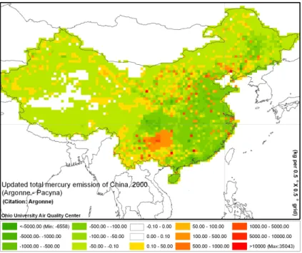
1. Pacyna: Anthropogenic emissions derived from Pacyna et al. (2006). 20

2. No China: Same asPacynabut with anthropogenic emissions from China set to zero.

3. Streets: Same as Pacyna but with emissions from China based on Streets et al. (2005).

The No Chinaand the Streets cases had identical emissions except for China. The 25

(7)

ACPD

8, 19861–19890, 2008

Title Page

Tables Figures

◭ ◮

Back Close

Full Screen / Esc

Interactive Discussion difference between Streets et al. (2005) emissions and Pacyna et al. (2006) emissions

for China. For all Hg sources in China, Streets et al. (2005) estimated 16.5% lower emissions. Total annual anthropogenic emissions for the three cases were as follows: 2207 Mg y−1_{for the}_Pacyna_{case, 1578 Mg y}−1_{for the}_{No China}_{case, and 1935 Mg y}1 for theStreetscase. Initial conditions of background Hg concentrations were assumed 5

to be 1.5 ng m−3_{(Ebinghaus et al., 2001; Weiss-Penzias et al., 2003; Swartzendruber} et al., 2006) in the form of Hg(0), distributed evenly over Earth’s surface and through all layers of the atmosphere (Slemr et al., 1985). Background concentrations of HGO were set to zero initially, because HGO has a short lifetime, and the model reaches steady state quickly.

10

3 Results

3.1 Elemental mercury

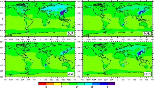
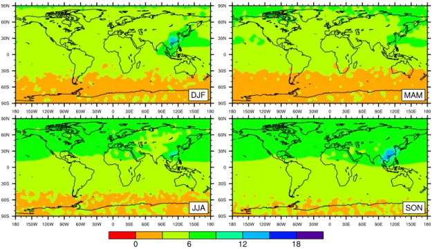
The global background concentrations of Hg(0) calculated by our model are shown in Fig. 2 for the Pacyna emissions case, as described in Sect. 2.3. Model results are shown for surface grid levels as averages for the four Northern Hemisphere seasons of 15

winter, spring, summer, and fall. For all seasons, concentrations of Hg(0) were highest for China, with values of 4 ng m−3 _{and more. Much of the Northern Hemisphere} ex-periences concentrations on the order of 2–3 ng m−3 _{during winter and fall. Seasonal} trends show the greatest Hg(0) concentrations during winter and the smallest concen-trations in summer, consistent with previous observations (Iverfeldt, 1991; Ames et 20

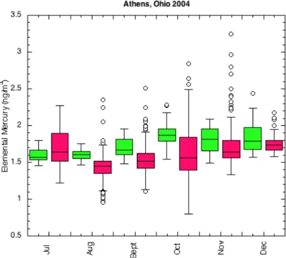
al., 1998; Ebinghaus et al., 2001; Kellerhals et al., 2003; Poissant et al., 2005; Sta-menkovic et al., 2007). Figure 3 compares model-calculated and measured Hg(0) in July–December 2004 at a site in the central Ohio River valley in Athens, Ohio (Yatavelli et al., 2006). The site is at approximately 900 ft above sea level and is on a small hill, at a height of 250 ft above the surrounding terrain. The model results shown are for a grid 25

(8)

ACPD

8, 19861–19890, 2008

Title Page

Tables Figures

◭ ◮

Back Close

Full Screen / Esc

Interactive Discussion the model-calculated concentrations are higher than measured values but within the

range of the measurement variability.

Figure 4 shows the percent di_fference in surface concentrations of Hg(0) between the Streets and No China simulations. Although the greatest difference is centered near and over China, evidence of transport in the Northern Hemisphere is suggested 5

by the ubiquitous increases in Hg(0), with more widespread transport during spring and summer. The spring transport causes Hg(0) concentrations to increase by up to 7% in parts of the western United States and 3–5% in the eastern United States. Background concentrations in the Southern Hemisphere are also a_ffected, although the e_ffect is small, with an increase of less than 1%. The average increase in Hg concentrations 10

globally is 3–4%.

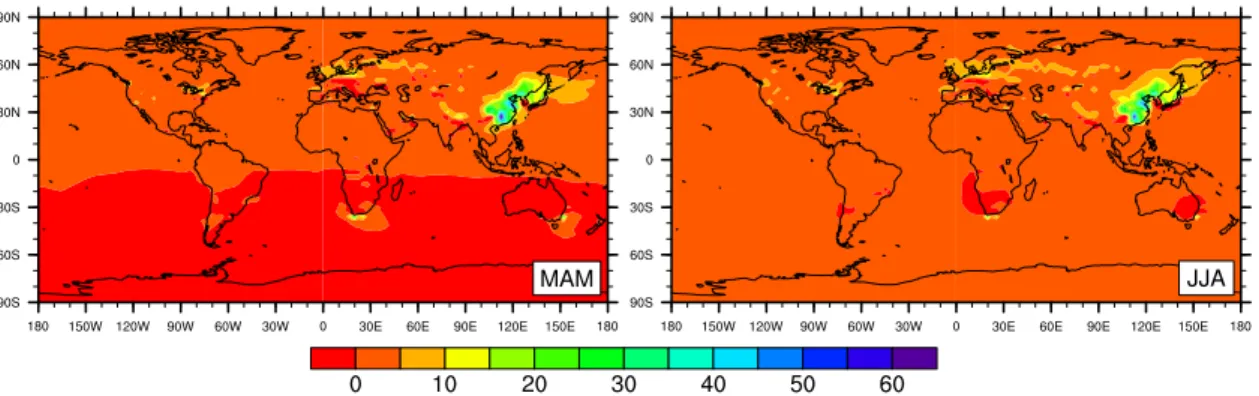
Comparison of thePacynaandStreetssimulations (Fig. 5) also indicates an increase in percent difference of Hg concentrations, although the increase is smaller than for the Streets and No China comparison (Fig. 4). In spring and summer, patterns for thePacyna-Streets comparison (Fig. 5) are similar to those for theStreets-No China 15

comparison (Fig. 4), with an increase in concentrations that extends throughout the Northern Hemisphere and smaller increases in the Southern Hemisphere. The vari-ability of Hg concentration in South Africa, Australia, and Europe (Fig. 5) is the result of differences in gridding the emission distribution input to MOZART. Although most of these effects are localized and most of the variations offset each other, they do have 20

an impact on the regional Hg budget. Nevertheless, the e_ffects do not make a large contribution to the global Hg budget (except for South Africa and Australia, where a few differences do not offset each other and cause an increase in Hg concentrations in excess of 1% in the Southern Hemisphere). For example, in the spring certain regions in the eastern United States have Hg concentrations that are 10% higher in thePacyna 25

simulation than inStreetssimulation. These pockets of high Hg concentration are small and occur near regions where anthropogenic emissions do not agree between the two simulations.

(9)

ACPD

8, 19861–19890, 2008

Title Page

Tables Figures

◭ ◮

Back Close

Full Screen / Esc

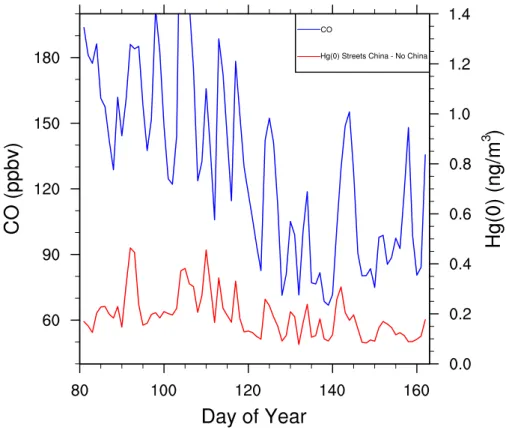
Interactive Discussion are emitted through industrial processes, have similar lifetimes, and can be transported

long distances in the atmosphere (Ja_ffe et al., 2005; Friedli et al., 2004; Weiss-Penzias et al., 2007). Figure 6 shows a time series for 22 March–10 June 2004, of calculated CO and Hg(0) concentrations near Okinawa. We chose this time period because it falls within the observations of Ja_ffe et al. (2005), and spring corresponds to peak con-5

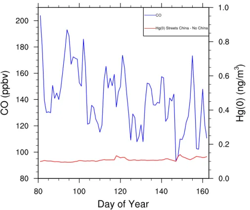
tinental outflow in the western Pacific. To improve representation of episodic transport events, we removed the contribution of background emissions by subtractingNo China Hg(0) fromStreetsHg(0). The largest transport events occurred in April and May, and several corresponded to events observed by Ja_ffe et al. (2005). For example, Ja_ffe et al. (2005) observed a large transport event on 20 April 2004 (day 111), while MOZART 10

calculated a transport event on 21 April 2004 (day 112). Figure 7 shows the same time series for a location near Seattle, Washington. In this case, subtraction of theNo ChinaHg(0) fromStreets Hg(0) revealed no episodic transport events. Mercury from China in the atmosphere seems to be fairly well mixed into the background when it has migrated this distance from the source.

15

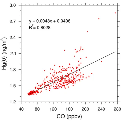
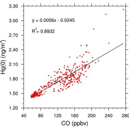
Figures 8 and 9 are plots of calculated concentration ratios (Hg(0):CO) from theNo China and Streets simulations, respectively. The slopes for the regression lines of these two graphs are 0.0043 ng m−3_ppbv−1 _{for the} _{No China} _{simulation (Fig. 8) and} 0.0056 ng m−3_ppbv−1_{for the}_Streets_{simulation (Fig. 9). These values correspond well} with results for observations of Jaffe et al. (2005) (slope=0.0053 ng m−3_ppbv−1_{) and} 20

the ACE-Asia field campaign (Friedli et al., 2004) (slope₌0.0056 ng m−3_ppbv−1_{). The} calculated values for Hg(0) and CO in Figs. 8 and 9 are well correlated, withR2values of 0.80 for theNo Chinasimulation and 0.89 for theStreetssimulation. The difference in the values for correlation of determination is caused by the variability of Hg(0), rather than CO, between simulations. Because Hg(0) was the only pollutant from China that 25

(10)

ACPD

8, 19861–19890, 2008

Title Page

Tables Figures

◭ ◮

Back Close

Full Screen / Esc

Interactive Discussion 3.2 Reactive mercury

To evaluate the model-calculated HGO, we analyzed wet and dry deposition, as dis-cussed below. Results from all the three scenarios disdis-cussed in Sect 2.3 are used for the analysis.

3.2.1 Wet deposition 5

Wet deposition is highly seasonal, being highest in spring and lowest in fall. Obser-vations suggest that wet deposition is usually low during winter in the United States. The calculated wet deposition is high during winter in MOZART simulations because of large concentrations of HGO at that time. Seasonal wet deposition di_fferences be-tween theStreetsandNo Chinasimulations are shown in Fig. 10. The differences are 10

concentrated over China, with evidence of global transport, particularly during the sum-mer. During winter and fall, decreased transport causes a large flux of HGO deposition over China. During spring and summer, strong winds allow Hg to cross the Pacific Ocean and become well mixed with the air in the Northern Hemisphere. Thus, during spring and summer an increase in wet deposition occurs throughout the entire North-15

ern Hemisphere. This increase in wet deposition amounts to 7–8% in the eastern and western United States, with larger changes in portions of the western United States. In the Southern Hemisphere, wet deposition of HGO increases globally by an average of 2%. The largest increase in deposition away from the source occurs in spring, when transport is strongest and outflow from western Pacific is dominant. However, the gen-20

erally greater wet deposition during this season makes the percent increases in wet deposition small. The opposite is true for the fall – though the amount of wet-deposited HGO changes little between simulations, the percent increase is large, because little wet deposition occurs in the fall.

Differences in wet deposition between thePacyna and Streets simulations for the 25

(11)

ACPD

8, 19861–19890, 2008

Title Page

Tables Figures

◭ ◮

Back Close

Full Screen / Esc

Interactive Discussion (Fig. 10), the biggest increase in emissions in thePacyna-Streetscomparison (Fig. 11)

occurs during the spring; however, the largest percent change occurs during the sum-mer because of the smaller wet deposition in sumsum-mer. Again, both seasons show transport, with wet deposition increases of 4% over the United States and Canada dur-ing the summer. Durdur-ing the sprdur-ing, the percent di_fference is 2% over the entire United 5

States. The Southern Hemisphere has a difference of less than 1–2%.

3.2.2 Dry deposition

Dry deposition patterns are very similar to the wet deposition patterns. In general, dry deposition peaks in spring in the Northern Hemisphere and in fall in the Southern Hemisphere.

10

For dry deposition, the percent difference between the Streets and No China sim-ulations is shown in Fig. 12. The largest percent change in dry deposition occurred over China during the winter and fall, when the year’s smallest outflow into the western Pacific allowed Hg to be deposited near its source. However, the change in dry depo-sition during the spring and summer showed a more global increase. Ready transport 15

across the Northern Hemisphere during these seasons allowed larger differences in deposition patterns between simulations, especially during the spring when transport is the highest. During the spring, di_fferences in dry deposition increased by 7–8% in the western United States and by 6–7% in the eastern United States. During the sum-mer, differences in dry deposition increased by 7–9% in the western United States, by 20

>9% in the far northwestern United States, and by 5–6% in the eastern United States. The change in dry deposition was generally less than 1% in the Southern Hemisphere. Although both summer and fall seasons showed large percent increases in dry depo-sition, absolute di_fferences betweenStreetsandNo Chinawere smallest during these months because of the low rates of dry deposition during this period (Sect. 3.3.1). Fig-25

(12)

ACPD

8, 19861–19890, 2008

Title Page

Tables Figures

◭ ◮

Back Close

Full Screen / Esc

Interactive Discussion occurred during spring, although the percent change was small because dry deposition

was high. During the summer, a more pronounced increase occurred, particularly over China, but the pattern also extended through the Pacific Ocean and into the northwest-ern United States. Spring increases in differences in dry deposition were 4% over the United States. During the summer, the percent change in dry deposition was much 5

greater in the northern United States (6%) than in the southern United States (4%). Increases in the Southern Hemisphere amounted to 1–2% for all seasons.

4 Conclusions

We used the chemical transport model MOZART with two additional constituents – Hg(0) and HGO – as transported species. The model was used to evaluate the sensi-10

tivity of calculated Hg(0) and HGO over the United States to anthropogenic emissions in China. The model-calculated Hg concentrations, in general, fell into the range of current observations. Concentrations of Hg(0) are seasonal, with high values during the winter and low values during the spring. Ratios of Hg(0):CO also show that the model does capture the relationship between Hg and the CO tracer, demonstrating the 15

model’s ability to simulate the correct Hg(0) pattern. Deposition of Hg is also seasonal, with peaks in the springtime and minimum values during the fall. With decreased or increased emissions from China, changes in concentration and deposition are expe-rienced globally. Large changes occur locally during winter and fall, and changes in transport occur during spring and summer. Including emissions from China in the sim-20

ulations increased calculated Hg concentrations in the United States by up to 7%. Uncertainties in Hg emissions and distribution (both anthropogenic and natural) are still significant, creating difficulties in estimating the circulation of Hg. Wu et al. (2006) found that Hg emissions from China are increasing at a rate of about 3% per year. In addition, the much higher Hg emission rates from China estimated by Jaffe et al. (2005) 25

(13)

er-ACPD

8, 19861–19890, 2008

Title Page

Tables Figures

◭ ◮

Back Close

Full Screen / Esc

Interactive Discussion rors in emission fractions. Some of the missing or underestimated emissions have been

accounted for as originating in natural sources, through an evaluation of emissions by vegetation, soil, and water by Shetty et al. (personal communication, 2008). Includ-ing these new estimates would lead to an increase in transport to the western United States, as well as an increase in the global background of Hg. Other studies have 5

demonstrated the effect of aqueous chemistry on Hg concentrations and deposition (Shia et al., 1999; Seigneur et al., 2006). Including aqueous chemistry can increase Hg(0) concentrations by a factor of 2–4 (Seigneur et al., 2006) and decrease wet and dry deposition of HGO by 18% and 9%, respectively (Shia et al., 1999). To improve understanding of the Hg cycle, we will address this chemistry and will also incorporate 10

a better estimate of Hg emissions in future work.

Acknowledgements. The work at Argonne National Laboratory was supported by the US De-partment of Energy, Office of Science, Office of Biological and Environmental Research, under contract DE-AC02-06CH11357.

References

15

Ames, M., Gullu, G., and Olmex, I.: Atmospheric mercury in the vapor phase, and in fine and coarse particulate matter at Perch River, New York, Atmos. Environ., 32, 865–872, 1998. Banic, C. M., Beauchamp, S. T., Tordon, R. J., Schroeder, W. H., Steffen, A., Anlauf, K. A., and

Wong, H. K. T.: Vertical distribution of gaseous Hg(0) in Canada, J. Geophys. Res., 108(D9), 4264, doi:10.1029/2002JD002116, 2003.

20

Bergan, T., Gallardo, L., and Rodhe, H.: Mercury in the global troposphere: A three-dimensional model study, Atmos. Environ., 33, 1575–1585, 1999.

Brasseur, G. P, Hauglustaine, D. A., Walters, S., Rasch, P. J., Muller, J.-F., Ganier,C., and Tie, X. X., MOZART: A global chemical transport model for ozone and related chemical tracers – Part 1, Model description, J. Geophys. Res., 103, 28 265–28 289,1998.

25

Dastoor, A. P. and Larocque, Y.: Global circulation of atmospheric mercury: A modeling study, Atmos. Environ., 38, 147–161, 2004.

(14)

ACPD

8, 19861–19890, 2008

Title Page Abstract Introduction Conclusions References Tables Figures ◭ ◮ ◭ ◮ Back Close

Full Screen / Esc

Interactive Discussion high time resolution: Recent application in environmental research and monitoring, Fresen,

J. Anal. Chem., 371, 806–815, 2001.

Friedli, H. R., Radke, L. F., Prescott, R., Li, P., Woo, J. H., and Carmichael, G. R.: Mercury in the atmosphere around Japan, Korea, and China as observed during the 2001 ACE-Asia field campaign: Measurements, distributions, sources, and implications, J. Geophys. Res., 5

109, D19S25, doi:10.1029/2003JD004244, 2004.

Giorgi F. and Chameides, W. L.: The rainout parameterization in a photochemical model, J. Geophys. Res., 90, 7872–7880, 1985.

Hack J. J.: Parameterization of moist convection in the National Center of Atmospheric Re-search Community Model (CCM2), J. Geophys. Res., 99, 5551–5568, 1994.

10

Hall, B.: The gas-phase oxidation of elemental mercury by ozone, Water Air Soil Poll., 80, 235–250, 1995.

Hall, B. and Bloom, N.: Report to EPRI, Electric Power Research Institute, Palo Alto, Calif., 1993.

Hauglustaine, D. A., Brasseur, G. P., Walters, S., Rasch, P. J., Muller, J.-F., Emmons, L. K., and 15

Carroll, M. A., MOZART: A global chemical transport model for ozone and related chemical tracers – Part 2: Models results and evaluations, J. Geophys. Res.,103, 28 291–28 335, 1988.

Holtslag, A. and B. Boville: Local versus nonlocal boundary-layer diffusion in a global climate model, J. Clim., 6, 1825–1842, 1993.

20

Horowitz, L. W., Walters, S., Mauzerall, D. L., Emmons, L. K., Rasch, P. J., Granier, C., Tie, X., Lamarque, J. F., Schultz, M. G., Tyndall, G. S., Orlando, J. J., and Brasseur, G. P.: A global simulation of tropospheric ozone and related tracers: Description and evaluation of MOZART, version 2, J. Geophys. Res., 108, 4784, doi:10.1029/2002JD002853, 2003. Iverfeldt, ˚A.: Occurrence and turnover of atmospheric mercury over the Nordic countries, Water 25

Air Soil Poll., 56, 251–265, 1991.

Jaffe, D., Prestbo, E., Swartzendruber, P., Weiss-Penzias, P., Kato, S., Takami, A., Hatakeyama, S., and Kajii, Y.: Export of atmospheric mercury from Asia, Atmos. Environ., 39, 3029–3038, 2005.

Kellerhals, M., Beauchamp, S., Belzer, W, Blanchard, P., Froude, F., Harvey, B., McDonald, 30

(15)

ACPD

8, 19861–19890, 2008

Full Screen / Esc

Interactive Discussion Lin, S.-J. and Rood, R. B.: Multidimensional flux-form semi-Lagrangian transport schemes,

Mon. Wea. Rev., 124, 2046–2070, 1996.

M ¨uller, J.-F. and Brassuer, G.: IMAGES: A three-dimensional chemical transport model for the global atmosphere, J. Geophys. Res., 100, 16 445–16 490, 1995.

National Research Council, Toxicological Effects of Methylmercury, Committee on the toxico-5

logical effects of Methylmercury, National Academy Press, Washington, DC, 2000.

Olivier, J. G. J., Bouwman, A. F.,van der Maas, C. W. M. , Berdowski, J. J. M., Veldt, C., Bloos, J. P. J., Visschedijk, A. J. H., Zandveld, P. Y. J., and Haverlag, J. L.: Description of EDGAR Ver-sion 2.0: A set of Global EmisVer-sion Inventories of Greenhouse Gases and Ozone-Depleting Substances for All Anthropogenic and Most Natural Sources on a Per Country Basis and on 10

a 1×1 degree grid, RIVM report 771060 002/TNO-MEP report R96/119, National Institute of Public Health and the Environment, Bilthoven, The Netherlands, 1996.

Pacyna, E. G., Pacyna, J. M., Steenhuisen, F., and Wilson, S.: Global anthropogenic mercury emission inventory for 2000, Atmos. Environ., 40, 4048–4063, 2006.

Pal., B. and Ariya, P. A.: Gas-phase HO-initiated reactions of elemental mercury: Kinetics, 15

product studies and atmospheric implications, Environ. Sci. Technol., 38, 5555–5566, 2004. Poissant, L., Pilote, M., Beauvais, C., Constant, P., and Zhang, H. H.: A year of continuous

measurements of three atmospheric mercury species (GEM, RGM, and Hgp) in southern

Quebec, Canada, Atmos. Environ., 39, 1275–1287, 2005.

Ryaboshapko, A., Bullock Jr., O. R., Christensen, J., Cohen, M., Dastoor, A., Ilyin, I., Peter-20

son, G., Syrakov, D., Travnikov, O., Artx, R. S., Davignon, D., Draxler, R. R., Munthe, J., and Pacyna, J.: Intercomparison study of atmospheric mercury models: 2. Modeling results vs. long-term observations and comparison of country deposition budgets, Sci. Total Envi-ron., 377, 319–333, 2007.

Seigneur, C., Karamchandani, P., Lohman, K., Vijayaraghavan, K., and Shia, R.-L.: Multiscale 25

modeling of the atmospheric fate and transport of mercury, J. Geophys. Res., 106(D21), 27 795–27 809, 2001.

Seigneur, C., Vijayaraghavan, K., Lohman, K., Karamchandani, P., and Scott, C.: Global source attribution for mercury deposition in the United States, Environ. Sci. Technol., 38(2), 555– 569, 2004.

30

(16)

ACPD

8, 19861–19890, 2008

Full Screen / Esc

Interactive Discussion Selin, N. E., Jacob, D. J., Park, R. J., Yantosca, R. M., Strode, S., Jaegle L., and Jaffe, D.:

Chemical cycling and deposition of atmospheric mercury: Global constraints from observa-tions, J. Geophys. Res., 112, D02308, doi:10.1029/2006JD007450, 2007.

Shia, R.-L., Seigneur, C., Pai, P., Ko, M., and Sze, N. D.: Global simulation of atmospheric mercury concentrations and deposition fluxes, J. Geophys. Res., 104, 23 747–23 760, 1999. 5

Slemr, F., Schuster, G., and Seiler, W.: Distribution, speciation, and budget of atmospheric mercury, J. Atmos. Chem., 3, 407–434, 1985.

Sommer, J., G ˚ardfeldt, K., Str ¨omberg, D., and Feng, X.: A kinetic study of the gas-phase reaction between the hydroxyl radical and atomic mercury, Atmos. Environ., 35, 3049–3054, 2001.

10

Stamenkovic, J., Lyman, S., and Gustin, M. S.: Seasonal and diel variation of atmospheric mercury concentrations in the Reno (Nevada, USA) airshed, Atmos. Environ., 41, 6662– 6672, 2007.

Steding, D. J. and Flegal, A. R.: Mercury concentrations in coastal California precipitation: evidence of local and trans-Pacific fluxes of mercury to North America, J. Geophys. Res., 15

107(D24), 4764, doi:10.1029/2002JD002081, 2002.

Streets, D. G., Jiming, H., Wu, Y., Jiang, J., Chan, M., Tian, H., and Feng, X.: Anthropogenic mercury emissions in China, Atmos. Environ., 39, 7789–7806, 2005.

Swartzendruber, P. C., Jaffe, D. A., Prestbo, E. M., Weiss-Penzias, P., Stelin, N. E., Park, R., Jacob, D. J., Strode, S., and Jaegle, L.: Observations of reactive gaseous mercury in 20

the free troposphere at the Mount Bachelor Observatory, J. Geophys. Res., 111, D24301, doi:10.1029/2006JD007415, 2006.

Tokos, J. S. S., Hall, B., Calhoun, J. A., and Prestbo, E. M.: Homogeneous gas-phase reaction of HGO with H₂O₂, O₃, CH₃I, and (CH₃)₂S: Implication for atmospheric Hg cycling, Atmos. Environ., 32, 823–827, 1998.

25

Travnikov, O. and Ryaboshapko, A.: Modelling of mercury hemispheric transport and deposi-tions. MSC-E Technical Report 6/2002, Meteorological Synthesizing Centre-East, Moscow, Russia, 67 pp., 2002.

Williamson D. L. and Rasch, P. J.: Two dimensional, semi-Lagrangian transport with shape preserving interpolation, Mon. Weather Rev., 117, 102–129, 1989.

30

(17)

ACPD

8, 19861–19890, 2008

Title Page

Tables Figures

◭ ◮

Back Close

Full Screen / Esc

Interactive Discussion Research, 108(D2), 8235, doi:10.1029/2001JD000772, 2003.

Weiss-Penzias, P., Jaffe, D. A., McClintick, A., Prestbo, E. M., and Landis, M. S.: Gaseous ele-mental mercury in the marine boundary layer: Evidence for rapid removal in anthropogenic pollution, Environ. Sci. Technol., 37, 3755–3763, 2003.

Weiss-Penzias, P., Jaffe, D., Swartzendruber, P., Hefner, W., Chanol, D., and Prestbo, E.: Quan-5

tifying Asian and biomass burning sources of mercury using the Hg/CO ratio in pollution plumes observed at the Mount Bachelor observatory, Atmos. Environ., 41(21), 4366–4379, 2007.

Wu, Y., Wang, S., Streets, D. G., Hao, J., Chan, M., and Jiang, J.: Trends in anthropogenic mercury emissions in China from 1995 to 2003, Environ. Sci. Technol., 40, 5312–5318, 10

2006.

Yatavelli, R. L. N., Fahrni, J. K., Kim, M., Crist, K. C., and Vickers, C. D.: Mercury, PM2.5 and gaseous co-pollutants in the Ohio River Valley region: Preliminary results from the Athens supersite, Atmos. Environ., 40, 6650–6665, 2006.

Zhang, G. J. and McFarlane, N. A.: Sensitivity of climate simulations to the parameterization 15

(18)

ACPD

8, 19861–19890, 2008

Title Page

Tables Figures

◭ ◮

Back Close

Full Screen / Esc

Interactive Discussion Fig. 1. Differences between the lower Streets et al. (2005) and higher Pacyna et al. (2006)

(19)

ACPD

8, 19861–19890, 2008

Title Page

Tables Figures

◭ ◮

Back Close

Full Screen / Esc

Interactive Discussion Fig. 2. Model-calculated background Hg(0) concentrations (ng m−3_{) at the model surface for}

(20)

ACPD

8, 19861–19890, 2008

Title Page

Tables Figures

◭ ◮

Back Close

Full Screen / Esc

Interactive Discussion Fig. 3. Observed and modeled concentrations of Hg(0) for a model grid located over Athens,

(21)

ACPD

8, 19861–19890, 2008

Title Page

Tables Figures

◭ ◮

Back Close

Full Screen / Esc

Interactive Discussion Fig. 4. Percent difference in Hg(0) concentrations between a simulation using the Hg(0)

(22)

ACPD

8, 19861–19890, 2008

Title Page

Tables Figures

◭ ◮

Back Close

Full Screen / Esc

Interactive Discussion Fig. 5. Percent difference in Hg(0) concentrations in spring (left) and summer (right), as

(23)

ACPD

8, 19861–19890, 2008

Title Page

Tables Figures

◭ ◮

Back Close

Full Screen / Esc

Interactive Discussion Fig. 6.Calculated concentrations of CO (ppbv) and Hg(0) (ng m−3_{) near Okinawa for the period}

(24)

ACPD

8, 19861–19890, 2008

Title Page

Tables Figures

◭ ◮

Back Close

Full Screen / Esc

Interactive Discussion Fig. 7.Calculated concentrations of CO (ppbv) and Hg(0) (ng m−3_{) near Seattle, Washington,}

(25)

ACPD

8, 19861–19890, 2008

Title Page

Tables Figures

◭ ◮

Back Close

Full Screen / Esc

Interactive Discussion Fig. 8. Scatter plot of calculated Hg(0) (ng m−3_{) vs. CO concentrations (ppbv) near Okinawa}

(26)

ACPD

8, 19861–19890, 2008

Title Page

Tables Figures

◭ ◮

Back Close

Full Screen / Esc

Interactive Discussion Fig. 9. Scatter plot of calculated Hg(0) (ng m−3_{) vs. CO (ppbv) concentrations near Okinawa}

(27)

ACPD

8, 19861–19890, 2008

Title Page

Tables Figures

◭ ◮

Back Close

Full Screen / Esc

Interactive Discussion Fig. 10. Percent differences in HGO wet deposition in winter (upper left), spring (upper right),

(28)

ACPD

8, 19861–19890, 2008

Title Page

Tables Figures

◭ ◮

Back Close

Full Screen / Esc

Interactive Discussion Fig. 11. Percent differences in HGO wet deposition in spring (left) and summer (right) for the

(29)

ACPD

8, 19861–19890, 2008

Title Page

Tables Figures

◭ ◮

Back Close

Full Screen / Esc

Interactive Discussion Fig. 12. Percent differences in HGO dry deposition in winter (upper left), spring (upper right),

(30)

ACPD

8, 19861–19890, 2008

Title Page

Tables Figures

◭ ◮

Back Close

Full Screen / Esc

Interactive Discussion Fig. 13. Percent differences in HGO dry deposition in spring (left) and summer (right) for the