A model study of the seasonal and long term North Atlantic surface <i>p</i>CO<sub>2</sub> variability

(1)

BGD

8, 10187–10227, 2011

North AtlanticpCO₂ variability

J. F. Tjiputra et al.

Title Page

Abstract Introduction

Conclusions References

Tables Figures

◭ ◮

Back Close

Full Screen / Esc

Printer-friendly Version

Interactive Discussion

Discussion

P

a

per

|

Dis

cussion

P

a

per

|

Discussion

P

a

per

|

Discussio

n

P

a

per

|

Biogeosciences Discuss., 8, 10187–10227, 2011 www.biogeosciences-discuss.net/8/10187/2011/ doi:10.5194/bgd-8-10187-2011

Biogeosciences Discussions

This discussion paper is/has been under review for the journal Biogeosciences (BG). Please refer to the corresponding final paper in BG if available.

A model study of the seasonal and long

term North Atlantic surface

p

CO

₂

variability

J. F. Tjiputra1,2, A. Olsen2,3, K. Assmann4, B. Pfeil1,2,5, and C. Heinze1,2,6

1

University of Bergen, Geophysical Institute, Bergen, Norway

2

Bjerknes Centre for Climate Research, Bergen, Norway

3

Institute of Marine Research, Bergen, Norway

4

British Antarctic Survey, Cambridge, UK

5

World Data Center for Marine Environmental Sciences, Bremen, Germany

6

Uni Bjerknes Centre, Uni Research, Bergen, Norway

Received: 30 September 2011 – Accepted: 9 October 2011 – Published: 20 October 2011 Correspondence to: J. F. Tjiputra (jerry.tjiputra@bjerknes.uib.no)

(2)

BGD

8, 10187–10227, 2011

Title Page

Tables Figures

◭ ◮

Back Close

Full Screen / Esc

Discussion

P

a

per

|

Dis

cussion

P

a

per

|

Discussion

P

a

per

|

Discussio

n

P

a

per

|

Abstract

A coupled biogeochemical-physical ocean model is used to study the long term varia-tions of surfacepCO₂ in the North Atlantic Ocean. The model agrees well with recent underwaypCO₂observations from the Surface Ocean CO₂Atlas (SOCAT) database in various locations in the North Atlantic. The distinct seasonal cycles observed at di_ff

er-5

ent parts of the North Atlantic are well reproduced by the model. In most regions except the subpolar domain, the recent observed trends inpCO₂ and air–sea carbon fluxes are also simulated by the model. Over a long period between 1960–2008, the primary mode of surfacepCO₂variability is dominated by the increasing trend associated with the invasion of anthropogenic CO₂ into the ocean. We show that, to first order, the

10

ocean surface circulation and air–sea heat flux patterns can explain the spatial vari-ability of this dominant increasing trend. Regions with strong surface mass transport and negative air–sea heat flux have the tendency to maintain lower surface pCO₂. Regions of surface convergence and mean positive air–sea heat flux such as the sub-tropical gyre and the western subpolar gyre have faster increase inpCO₂over a long

15

term period. The North Atlantic Oscillation (NAO) plays a major role in controlling the variability occurring at interannual to decadal time scales. The NAO predominantly in-fluences surfacepCO₂in the North Atlantic by changing the physical properties of the North Atlantic water masses, particularly by perturbing the temperature and dissolved inorganic carbon in the surface ocean. We show that present underway observations

20

(3)

BGD

8, 10187–10227, 2011

Title Page

Tables Figures

◭ ◮

Back Close

Full Screen / Esc

Discussion

P

a

per

|

Dis

cussion

P

a

per

|

Discussion

P

a

per

|

Discussio

n

P

a

per

|

1 Introduction

Future climate change will depend on the evolution of the atmospheric CO₂ concentra-tion, which has been perturbed considerably by human activity during the past cen-turies. Studies have confirmed that less than half of the total anthropogenic CO₂ emitted over the anthropocene era due to burning of fossil fuels, land use change,

5

and cement production remain in the atmosphere today (e.g., Canadell et al., 2007; Le Qu ´er ´e et al., 2009). The rest is taken up by the terrestrial and ocean reservoirs mainly through plant photosynthesis and dissolution into seawater, respectively. The anthropogenic carbon uptake rate, however, is inhomogeneous and depends strongly on other external forcings acting on different spatial and temporal scales. In the ocean,

10

the carbon uptake is influenced by processes ranging from short term biological activity to long term climate variability.

The North Atlantic ocean is an important region for oceanic carbon uptake. Taka-hashi et al. (2009) show that the most intense CO₂ sink area of the world oceans is located in the North Atlantic (for reference year 2000). Because of this many studies,

15

both observational and modeling, in the past decade have been dedicated to better un-derstand the variability of air–sea CO₂ fluxes in this region (e.g., Lef èvre et al., 2004; L üger et al., 2006; Corbi ère et al., 2007; Thomas et al., 2008; Ullman et al., 2009; Watson et al., 2009; McKinley et al., 2011). In addition to altering the physical prop-erties such as temperature and ocean circulation of the North Atlantic basin, climate

20

change will also feedback onto the biogeochemical processes by influencing the sur-face carbon chemistry and biological processes, crucial for the oceanic carbon uptake. Therefore, understanding the role of present climate variability in controlling the North Atlantic carbon uptake remains a fundamental challenge and a necessary step in order to reduce the uncertainty associated with future climate projections.

25

(4)

BGD

8, 10187–10227, 2011

Title Page

Tables Figures

◭ ◮

Back Close

Full Screen / Esc

Discussion

P

a

per

|

Dis

cussion

P

a

per

|

Discussion

P

a

per

|

Discussio

n

P

a

per

|

2009). For interannual and decadal timescales, the long term change in the physical parameters associated with ocean circulation and climate variability dominates. The leading mode of climate variability in the North Atlantic is the North Atlantic Oscillation (NAO) (Hurrell and Deser, 2009). In this study, we assess the seasonal variability of the surface pCO₂ simulated by an ocean biogeochemical general circulation model

5

(OBGCM) as compared to available observations. In addition, we apply a principal component statistical analysis to identify the primary and secondary mode of the sur-facepCO₂ variability over the North Atlantic basin over the 1960–2008 period. While the study by Thomas et al. (2008) has assessed the oceanic carbon uptake variability associated with the NAO, our study applies a different technique and covers a longer

10

period in time.

Since the partial pressure of surface CO₂(i.e.,pCO₂) is one of the carbon parame-ters that is directly measurable and can be closely linked to the oceanic carbon uptake, we focus on thepCO₂ for the comparison between model results and observations. Furthermore, with the advancement of measurement techniques, in the last few years,

15

autonomouspCO₂ measurement systems have been installed in many voluntary ob-serving ships (VOS) to monitor the seawaterpCO₂(Pierrot et al., 2009). Resulting from this is substantial increase in the number of ship-based surfacepCO₂measurements with relatively high coverage both in space and time (Watson et al., 2009). In certain regions, the number of ship tracks increase to a point where month-to-month

measure-20

ments can be compiled. This allows further insight into understanding the spatial and temporal variations of carbon dynamics in the North Atlantic region.

Another motivation for this study is to evaluate whether or not the governing pro-cesses behind the ocean carbon cycle model used in this study are su_fficient to sim-ulate the observed spatial and temporalpCO₂ variability in the North Atlantic.

Basin-25

(5)

BGD

8, 10187–10227, 2011

Title Page

Tables Figures

◭ ◮

Back Close

Full Screen / Esc

Discussion

P

a

per

|

Dis

cussion

P

a

per

|

Discussion

P

a

per

|

Discussio

n

P

a

per

|

and provide more confidence in future projections of the climate system and its associ-ated carbon cycle feedback. It also serves as a prerequisite to test whether the model provides an appropriate first guess for use in advanced data assimilation schemes for more detailed global and regional predictions and optimisation of governing parameters of the carbon cycle.

5

The paper is organized as follows: in the next two sections we describe the observa-tions and model used in this study. Section four discusses the results of the experiment analysis, and the study is summarized in section five.

2 Observation

In order to evaluate the model simulation, two independent data sets are employed.

10

The first is from the CARINA (CARbon dioxide IN the Atlantic Ocean) data synthesis project which can be downloaded from http://cdiac.ornl.gov/oceans/CARINA/ (Velo et al., 2009; Key et al., 2010; Pierrot et al., 2010; Tanhua et al., 2010). It is comprised of quality-controlled observation from 188 cruises focusing on carbon-related parameters. For the model comparison, we extracted the surface measurements of temperature

15

(SST), salinity (SSS), dissolved inorganic carbon (DIC), and alkalinity (ALK) over the North Atlantic domain between 1990 and 2006. The data is then averaged and binned into monthly fields with 1◦_{by 1}◦_{horizontal resolution.}

The second data set are observations of underway surface fCO₂ (i.e., fugacity of CO₂) extracted from the Surface Ocean CO₂Atlas (SOCAT, Pfeil et al., 2011). SOCAT

20

is the latest and most comprehensive surface oceanfCO₂ data base, containing 6.3 millionfCO₂values from 1851 voyages carried out during the time span between 1968 and 2007. SOCAT contains only measured fCO₂ data (i.e., not calculated from, for example, dissolved inorganic carbon and total alkalinity data). The data have been predominantly analyzed through infrared analysis of a sample of air in equilibration

25

(6)

BGD

8, 10187–10227, 2011

Title Page

Tables Figures

◭ ◮

Back Close

Full Screen / Esc

Discussion

P

a

per

|

Dis

cussion

P

a

per

|

Discussion

P

a

per

|

Discussio

n

P

a

per

|

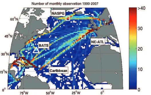
In this study, we focus on the data sub-set from the North Atlantic basin. Figure 1 shows all the ship tracks that contain some measurements. Since the data is mainly used for comparison with the model in the seasonal time scale, we isolate regions with a good seasonal (i.e., at least 8 out of 12 months) coverage over continuous years. In addition, we also avoid regions close to the continental margins where the

5

model does not perform adequately due to its fairly coarse resolution. Based on these criteria, we found three regions, each within a 4◦by 4◦horizontal domain (as shown by the white rectangle in Fig. 1), with reasonable seasonal coverage. To standardize the analysis, we use all data from these three locations spanning the 2002 to 2007 period for comparison with the model simulation.

10

The first region, centered at 60◦_{N 32}◦_{W, is located in the subpolar gyre (NASPG) and} was mainly covered by the routes of MV Skogafoss (processed by the United States, http://www.aoml.noaa.gov/ocd/gcc/skogafoss introduction.php) and MV Nuka Arctica of the Danish Royal Arctic Lines (Olsen et al., 2008). The second region is located in the Northeast North Atlantic and was covered by the several VOS lines operated by

15

Germany (Steinhoff, 2010), France, Spain (Gonz ´alez D ´avila et al., 2005; Padin et al., 2010), the UK (Schuster and Watson, 2007) and the United States, and is centered at 44◦_{N 17}◦_{W (NE-ATL). The last location is close to the Caribbean and is covered by} routes of reserch vessels from Germany, United States, Spain, and the UK, centered at 22◦_{N 52}◦_{W (Caribbean). The three sub-domains represent di}_ff_{erent types of oceanic}

20

provinces from low- to high-latitudes.

In addition to underway observations, thepCO₂data set from the Bermuda Atlantic Time series Station (BATS, 31◦₄₀′′_{N, 64}◦₁₀′′_{W) (Bates, 2007) is also used as} addi-tional model validation. The addition of BATS is useful as it is one of the best studied ocean locations. For the purpose of this study, we only use data from the same period

25

(7)

BGD

8, 10187–10227, 2011

Title Page

Tables Figures

◭ ◮

Back Close

Full Screen / Esc

Discussion

P

a

per

|

Dis

cussion

P

a

per

|

Discussion

P

a

per

|

Discussio

n

P

a

per

|

3 Model

In this study, we use a global coupled physical–biogeochemical ocean model (Assmann et al., 2010). The physical component is the dynamical isopycnic vertical coordinate MICOM ocean model (Bleck and Smith, 1990; Bleck et al., 1992), which includes some modifications as described in Bentsen et al. (2004). The horizontal resolution is

ap-5

proximately 2.4◦×2.4◦with grid spacing ranging from 60 km in the Arctic and Southern Ocean to 180 km in the subtropical regions. Vertically, the model consists of 34 isopy-cnic layers. In the additional topmost layer, the model adopts a single non-isopyisopy-cnic surface mixed layer, and its depth is computed according to formulation by Gaspar (1988). This temporally and spatially varying mixed layer provides the linkage between

10

the atmospheric forcing and the ocean interior.

The ocean carbon cycle model is the Hamburg Oceanic Carbon Cycle (HAMOCC5) model, which is based on the original work of Maier-Reimer (1993). The model has since then been improved extensively and has been used in many studies (Six and Maier-Reimer, 1996; Heinze et al., 1999; Aumont et al., 2003; Maier-Reimer et al.,

15

2005). The current version of the model includes an NPZD-type ecosystem model, a 12-layer sediment module, full carbon chemistry, and multi-nutrient co-limitation of the primary production. The surface pCO₂ in the model is computed based on the prognostic temperature, salinity, pressure, dissolved inorganic carbon, and alkalinity. For the air–sea gas exchange, the model adopts the formulation of Wanninkhof (1992).

20

A detailed description of the isopycnic version of HAMOCC is given by Assmann et al. (2010).

The model simulations performed in this study are forced by the daily atmospheric fields from the NCEP Reanalysis data set (Kalnay et al., 1996). For the air–sea CO₂ flux computation, the model prescribes observed atmospheric CO₂concentration

(in-25

(8)

BGD

8, 10187–10227, 2011

Title Page

Tables Figures

◭ ◮

Back Close

Full Screen / Esc

Discussion

P

a

per

|

Dis

cussion

P

a

per

|

Discussion

P

a

per

|

Discussio

n

P

a

per

|

SST in all three North Atlantic locations as well as BATS (supplement Fig. 1). During winter the model tends to have a deeper mixed layer depth (MLD) than is observed, which may be attributed to the slightly cooler SST as compared to the observation. A more detailed evaluation of the model performance with respect to the global physi-cal and carbon cycle parameters is also documented in Assmann et al. (2010).

5

4 Results

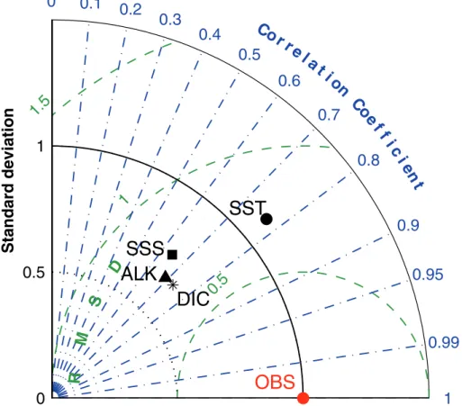
For the basin scale comparison with the CARINA data, the model-data fit is summa-rized in a Taylor diagram (Taylor et al., 2001) shown in Fig. 2. The Taylor diagram gives a statistical summary of how well the model simulated tracer distributions match the observed ones in term of correlation, standard deviations, and

root-mean-square-10

di_fference (RMSD). Note that we only apply the surface data set (five meter and above) for this comparison because the main focus of this study is to study the surfacepCO₂ variability. Figure 2 shows that the model simulated temporal and regional variabili-ties are generally close to the observation. The model simulated SST, SSS, DIC and ALK distributions have significant (within 95 % confidence interval) correlations of 0.77,

15

0.65, 0.73, and 0.69, respectively with the observations.

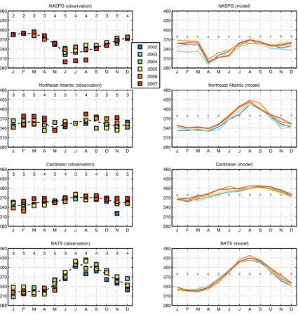
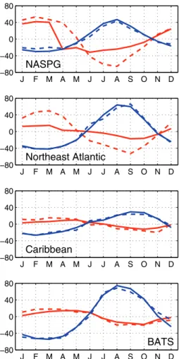
4.1 Regional seasonality offCO2

In this subsection we analyze the surface fCO₂ seasonal variability for the di_fferent sub-domains in the North Atlantic. The model simulatedpCO₂is converted intofCO₂ by using a conversion factor of 0.3 % (Weiss, 1974). Figure 3 compares the seasonal

20

(9)

BGD

8, 10187–10227, 2011

Title Page

Tables Figures

◭ ◮

Back Close

Full Screen / Esc

Discussion

P

a

per

|

Dis

cussion

P

a

per

|

Discussion

P

a

per

|

Discussio

n

P

a

per

|

To further identify the sources of the differences in seasonal variability between the model and data, we also separate the fCO₂ variability into temperature-driven (fCO₂-T) and non temperature-driven (fCO₂-nonT) variability following Takahashi et al. (2002). ThefCO₂-T represents the temperature-controlled variability, as colder wa-ter has higher CO₂solubility, thus lowerfCO₂, whereas the opposite is true for warmer

5

water. ThefCO₂-nonT is composed of variability associated with alkalinity, SSS, and DIC variations throughout the year. Anomalies of both the fCO₂-T and fCO₂-nonT monthly variability from the observations and model are shown in Fig. 4 for each stud-ied region.

For the NASPG region, the observations indicate a clear seasonal signal with winter

10

maximum and summer minimum, consistent with earlier analyses (Olsen et al., 2008) for this region. The model also simulates pronounced seasonal variations with an am-plitude close to the observations, but with its seasonal phase shifted by approximately two months. Based on the observations, Olsen et al. (2008) describe that the seasonal variability in this location is mostly dominated by upward mixing of DIC-rich water to

15

the surface in the winter and by strong biological consumption throughout spring and summer. Consistently, Fig. 4 also shows similar observed patterns, with a weaker am-plitude of the variability forfCO₂-T thanfCO₂-nonT in the NASPG. The model shows good agreement with the observations in terms offCO₂-T variability. ThefCO₂-nonT phase-shift in the model is predominantly attributed to the simulated timing and

dy-20

namic of biological processes. In the early spring period, the increase in tempera-ture and light availability lead to an accelerated simulated phytoplankton growth, which immediately consumes most of the nutrient upwelled during the previous winter. As a result, the nutrients become depleted and weak nutrient regeneration over the sum-mer season is insufficient to maintain the steady biological consumption as observed

25

(10)

BGD

8, 10187–10227, 2011

Title Page

Tables Figures

◭ ◮

Back Close

Full Screen / Esc

Discussion

P

a

per

|

Dis

cussion

P

a

per

|

Discussion

P

a

per

|

Discussio

n

P

a

per

|

the summer and dominates the increasing summer temperature. Consistent with the observations shown here, they found minimum fCO₂ values between 325–340 µatm during the summer. Simulating the correct ecosystem dynamics at high latitudes is a well known problem in global models as most models calibrate their ecosystem model towards time-series stations such as BATS, which are biased toward the subtropical

5

regions (Tjiputra et al., 2007). A recent one-dimensional ecosystem model study by Signorini et al. (2011) shows that more sophisticated multi-functional groups of phyto-plankton may be necessary to reproduce the biological carbon uptake during summer in the Icelandic waters close to where the NASPG domain is located.

The Northeast Atlantic station is located in between the North Atlantic subpolar and

10

subtropical gyres. It is therefore expected that the variability here is dominated by both temperature variability as well as surface DIC dynamics. The observations suggest that the fCO₂-T and fCO₂-nonT variability are equally important and nearly cancel each other resulting in a relatively weak seasonal cycle (e.g., compared to that in the sub-polar region), as shown in Fig. 3. The study by Schuster and Watson (2007) over

15

a somewhat larger ship-based observational region (30◦W–5◦W and 39◦N–50◦N) also shows similar weak seasonal fCO₂ variability in the early 2000s. The observations show two time intervals with maximum fCO₂: during late winter and late summer. Figure 4 shows that the late winter maximum is associated to the dynamics of surface DIC (nonT e_ffect) whereas the late summer maximum is dominated by the temperature

20

variations (i.e., maximum SST around the August and September months). The model is able to simulate the observedfCO₂-T seasonal cycle relatively well but the simulated

fCO₂-nonT is considerably weaker. The model fCO₂ variability in this location looks very similar to that at the BATS station (see Fig. 4). As described above, this artefact is potentially due to the ecosystem dynamics biased toward the one at BATS. Another

25

(11)

BGD

8, 10187–10227, 2011

Title Page

Tables Figures

◭ ◮

Back Close

Full Screen / Esc

Discussion

P

a

per

|

Dis

cussion

P

a

per

|

Discussion

P

a

per

|

Discussio

n

P

a

per

|

In the Caribbean sub-domain, both model and observations show the lowest sea-sonal variability of surface fCO₂ as compared to the other regions (Fig. 3). This is a general feature for low latitude regions (e.g., Watson et al., 2009). Figure 4 shows that variations in surface temperature are the main driver for the seasonal fluctuations, consistent with an earlier observational study over the same domain (Wanninkhof et al.,

5

2007). Consequently, maximum surfacefCO₂occurs in the summer period when SST is high, and the minimumfCO₂ is observed during winter. The smaller role of fCO₂ -nonT in this location can be attributed to the relatively weak seasonal variations in both the observed chlorophyll (i.e., biological activity) and mixed layer depth (Behrenfeld et al., 2005; de Boyer Mont ´egut et al., 2004).

10

A study by Bates et al. (1996) reported that the surface waters at BATS are super-saturated with respect to CO₂during the stratified summer months and undersaturated during the strong mixing in wintertime. Figure 3 shows that the model is able to sim-ulate the observed mean seasonal variability in terms of both phase and amplitude. While there is a pronounced seasonality in the surface DIC (i.e., upwelling of DIC-rich

15

subsurface water mass during the winter and biological production in the summer), both the model and observations agree in that the fCO₂-T variability dominates the seasonal variations (see Fig. 4). The seasonal SST variation at BATS is as large as that in the NASPG but the seasonal Net Primary Production (NPP) cycle remains much weaker (as shown in Supplemental Figs. 1 and 2). This dominant control of SST on

20

the surfacefCO₂at BATS has also been shown by Gruber at al. (2002) for the period prior to the year 2000. Thus, similar to the Caribbean station, thefCO₂-nonT at BATS has only minor contributions.

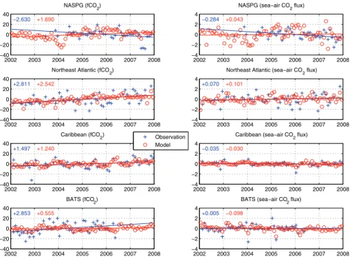
4.2 Regional trends infCO2and sea-air CO2flux

In this subsection, we compare the model simulated trend with estimates from

observa-25

(12)

BGD

8, 10187–10227, 2011

Title Page

Tables Figures

◭ ◮

Back Close

Full Screen / Esc

Discussion

P

a

per

|

Dis

cussion

P

a

per

|

Discussion

P

a

per

|

Discussio

n

P

a

per

|

seasonally filtered) by substracting the monthly mean values from the data sets. We estimate the CO₂ flux from the observations following the formulation of Wanninkhof (1992), and the CO₂solubility formulation of Weiss (1974). In situ SST and SSS are used for the solubility computation. When SSS is unavailable, a climatology from the World Ocean Atlas (WOA) data is used. NCEP monthly wind speed is used to

com-5

pute the gas transfer rate. Finally, monthly atmospheric CO₂concentration observed at Mauna Loa observatory is applied as a proxy of atmosphericpCO₂boundary condition over each stations.

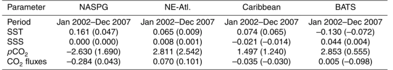
Table 1 shows that both the observations and the model consistently produce the same trend signals for SST and SSS, though the magnitude is weaker in the model.

10

As decribed in Assmann et al. (2010), in order for the model to maintain a stable and realistic Atlantic Meridional Overturning Circulation (AMOC), a Newtonian relaxation is applied to the SST and SSS parameters in the model. For the simulation in this study, the SST and SSS ate relaxed at time scales of 180 and 60 days, respectively. This may explains the much weaker trend simulated by the model as compared to the

15

observations, particularly for SSS. For most stations, except BATS, warming trends are estimated by both the model and the observations. There are only small changes in the surface salinity in all stations.

The seasonally filtered trends of surface fCO₂ and sea-air CO₂ fluxes in the four locations of North Atlantic are shown in Fig. 5. After the seasonal signals are removed

20

from the time-series, the model’s amplitude of the interannual variability agrees rea-sonably well with the observations, with higher variability being more pronounced in high latitudes. Both the model and the observations suggest that surfacefCO₂ inter-annual variability ranges within_±30 µatm for nearly all regions. The amplitude of the interannual variability of the sea-air CO₂fluxes varies from one region to the other, with

25

the strongest variability shown at high latitude (i.e., NASPG), and the weakest at low latitude (i.e., Caribbean).

(13)

BGD

8, 10187–10227, 2011

Title Page

Tables Figures

◭ ◮

Back Close

Full Screen / Esc

Discussion

P

a

per

|

Dis

cussion

P

a

per

|

Discussion

P

a

per

|

Discussio

n

P

a

per

|

where the observations indicate a negative trend. This is interesting as a previous study estimated that the surfacefCO₂ around the NASPG domain has increased relatively faster (e.g., over 1990–2006 period) than in other regions in the North Atlantic (Corbi `ere et al., 2007; Schuster et al., 2009). The observed negative trend in the NASPG domain can be attributed to the unusually low summerfCO₂ in 2007, which is not reproduced

5

by the model. This anomalously low fCO₂ value is recorded despite the fact that both model and observation indicate a positive anomaly in SST (not shown) during the summer of 2007 relative to the previous summer periods, as also shown in Table 1 (i.e., a warming trend in SST). Therefore, the anomalously low summerfCO₂in 2007 may be attributed to the other factors, such as the unusually high summer biological

10

production as seen from observationally-derived estimates (Behrenfeld and Falkowski, 1997). And due to the model deficiency in maintaining high summer productivity in this location (supplement Fig. 2), it is unable to reproduce the anomalously lowfCO₂value. Interestingly, a modeling study by Oschlies (2001) suggests only a small increase in the nutrient concentration in this region under a positive NAO-phase (2007 is a dominant

15

positive NAO phase year).

The respective observed atmospheric CO₂ trend for the same period is 2.031 ppm yr−1_{. Due to this opposing trend, it is not surprising that the observed} sea-air carbon flux in the NASPG has a large negative trend (i.e., larger ocean carbon uptake) of−0.284 mol C m−2yr−1. The model on the other hand suggests a very small

20

positive trend (i.e., less uptake) despite lower increase in surface oceanpCO₂than in atmospheric. This is partially attributed by the negative trend in the spring surface wind speed in the region (not shown), which leads the model to simulate weaker atmospheric carbon uptake over time. Note that for the NASPG location, the model simulates the largest sea-airfCO₂di_fference during the spring season as shown in Fig. 3.

25

At the Northeast Atlantic and Caribbean stations, the simulated positive surface

(14)

BGD

8, 10187–10227, 2011

Title Page

Tables Figures

◭ ◮

Back Close

Full Screen / Esc

Discussion

P

a

per

|

Dis

cussion

P

a

per

|

Discussion

P

a

per

|

Discussio

n

P

a

per

|

fluxes (see Fig. 5). At the Caribbean station, the fCO₂ trends are weaker than the atmospheric value and therefore the CO₂ fluxes are weakly decreasing as well. The opposing signals in CO₂fluxes between the two regions are also consistent with a re-cent observational-based estimate (covering a broader spectrum of VOS ship tracks between northwestern Europe and the Caribbean) that suggest a positive trend in

car-5

bon uptake followed by a negative one over the 2002–2007 period (Watson et al., 2009), resulting in small net change over the region.

The fCO₂ trends at BATS computed from the measurements and the model are both positive. However, the signal is much stronger in the observations, resulting in a negative trend in oceanic carbon sink. The modelfCO₂trend, on the other hand, is

10

weaker than the corresponding atmospheric trend, and the model therefore simulates increasing carbon uptake in this location. Consistent with our model result, a study by Ullman et al. (2009) also suggests a relatively smaller increase in surfacepCO₂at the BATS station compared to the rest of the North Atlantic region, although their trend extends over the 1992–2006 period.

15

4.3 Basin scale trends and variability

Previous subsections show that, despite its deficiencies, the model is able to reason-ably capture the seasonal variability and short-term trends observed in di_fferent re-gions in the North Atlantic basin. Here, we attempt to explain the regional variations in the surfacepCO₂ simulated by the model and, to some extent, the observed ones.

20

First, we analyze the dominant primary and secondary modes of long-term interannual variability of simulated surfacepCO₂ over the 1960–2008 period. To do this, we first removed the meanpCO₂value from each model grid point to yield the simulatedpCO₂ anomaly. A principal component statistical analysis (von Storch and Zwiers, 2002) was then applied to these anomalies. Figure 6 shows the first empirical orthogonal function

25

(EOF1) and the associated principal component (PC1) of the simulated annual surface

(15)

BGD

8, 10187–10227, 2011

Title Page

Tables Figures

◭ ◮

Back Close

Full Screen / Esc

Discussion

P

a

per

|

Dis

cussion

P

a

per

|

Discussion

P

a

per

|

Discussio

n

P

a

per

|

model simulated annual pCO₂ and atmospheric CO₂ concentration observed at the Mauna Loa station. Multiplying the EOF1 value with the PC1 time-series yields the pri-mary mode of surfacepCO₂variability simulated by the model. The temporal variability of PC1 indicates a dominant positive trend that correlates strongly with the observed atmospheric CO₂anomaly (r₌0.99). This suggests that the primary temporal

variabil-5

ity of surfacepCO₂ in the model is mainly due to the anthropogenic carbon invasion into the seawater. Therefore, at regional scales and in the long run, the oceanpCO₂ follows the atmosphere.

For the above reason, the EOF1 map shown in Fig. 6 indicates regions where the anthropogenic CO₂ significantly affects the surface pCO₂ concentration. The main

10

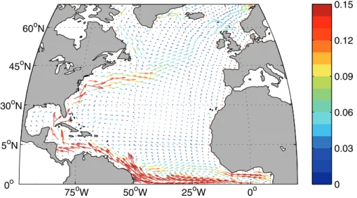
reason for the regional di_fferences in the magnitude of surfacepCO₂ increasing trend can be explained by the surface transport and air–sea heat flux patterns. The anthro-pogenic carbon taken up by the surface ocean is advected by the ocean circulation at the surface and transported into the deep by mixing and deep water formation pro-cesses (Tjiputra et al., 2010b). Figures 7 and 8 show the mean lateral ocean surface

15

velocity and air–sea heat flux simulated by the model over the 1960–2008 period. In regions with strong mass transport, such as the Gulf Stream, the relatively warm water mass from the subtropic is advected northward and looses heat to the atmosphere. Here, the cooling of surface temperature increases the CO₂ gas solubility and trans-lates into lower surfacepCO₂for the same dissolved inorganic carbon content. Thus,

20

along the 30◦_{N and 45}◦_{N, where the water is continuously transported northeastward} into the Nordic Seas by the North Atlantic drift water, the surfacepCO₂ increases rel-atively slower than the atmospheric CO₂ as illustrated in Fig. 6. In contrast, in the western subpolar gyre along 50◦_{N latitude, the water mass here is transported} south-ward from the Labrador Sea and warmed up by the atmosphere. Hence, the surface

25

pCO₂in this region increases relatively faster than the atmospheric CO₂.

(16)

BGD

8, 10187–10227, 2011

Title Page

Tables Figures

◭ ◮

Back Close

Full Screen / Esc

Discussion

P

a

per

|

Dis

cussion

P

a

per

|

Discussion

P

a

per

|

Discussio

n

P

a

per

|

such as the subtropical Atlantic convergence zone is marked by a stronger increase in surfacepCO₂ as less anthropogenic CO₂ is laterally advected away from this area (Fig. 7) and there is a net heat gain in this region (Fig. 8). Both the Greenland and the Norwegian Seas represent some of the oldest surface water masses before they are transported to the deep water (i.e., have resided for a long period close to the

5

sea surface), which also explains the relatively high anthropogenic CO₂concentration simulated in the model. On the western coast of North Africa, the anomalously lower contribution of anthropogenic CO₂can be explained by the fact that this is an upwelling region, where the water mass is less exposed to the anthropogenic CO₂.

The magnitude of PC1 shown in Fig. 6b is standardized to be comparable to the

10

observed atmospheric CO₂ anomaly. Therefore, the map of EOF1 can be used to approximate the strength of increasing surfacepCO₂trend relative to the atmospheric CO₂ trend. Values greater (less) than one suggest increasing surface pCO₂ faster (slower) than the atmospheric CO₂ partial pressure. Note that this trend and these variations occur over a much longer period than recent observational studies. Thus,

15

in order to understand and compare the trend in this study with relatively shorter trend resulted from the observational study, a further analysis on the short term interannual climate variability is required.

To understand the shorter term mode variability, we compute the second mode vari-ability simulated by the model. Figure 9 shows the EOF2, which gives the dominant

20

variability of surfacepCO₂after the positive trend resulting from the anthropogenic CO₂ uptake (see Fig. 6b) is removed. Thus it explains the main variations due to physical climate variability over the 1960–2008 period. Figure 9b shows that the temporal vari-ations of PC2 is reasonably well correlated with the North Atlantic Oscillation (NAO)-index (Hurrell and Deser, 2009) (r₌0.557). The NAO is a leading climate variability

25

(17)

BGD

8, 10187–10227, 2011

Title Page

Tables Figures

◭ ◮

Back Close

Full Screen / Esc

Discussion

P

a

per

|

Dis

cussion

P

a

per

|

Discussion

P

a

per

|

Discussio

n

P

a

per

|

which shows that changes in wind-driven ocean circulation associated with the NAO variability influence the North Atlantic CO₂ system by altering the surface water prop-erties.

The spatial pattern of EOF2 shown in Fig. 9 indicates that the second mode vari-ability (approximately NAO-like) predominantly represents the interannual varivari-ability of

5

surfacepCO₂in the North Atlantic sub-polar region, with opposite variability between the western and eastern parts. In the western sub-polar gyre, the model simulates pos-itive anomalies ofpCO₂under positive NAO condition, whereas the negative anomalies is simulated in the eastern part of the sub-polar gyre.

In the model, thepCO₂ is determined as a function of surface temperature (SST),

10

salinity (SSS), alkalinity, and dissolved inorganic carbon (DIC) concentrations. To quan-tify the influence of the NAO-variability on each of these parameters, we analyzed an earlier model simulation, which used the same atmospheric physical forcing, but main-tained a preindustrial atmospheric CO₂ concentration (Assmann et al., 2010). This simulation, in principle, would have the positive pCO₂ trend associated with the

an-15

thropogenic effects, as shown in Fig. 6, removed from the system. Therefore, it can be better used to analyze the variability of the CO₂system associated with the present climate variability. Next, we compute mean annual anomalies of the simulated SST, SSS, alkalinity, and DIC under the dominant positive and negative NAO phases be-tween 1960–2007. The dominant NAO-phase is defined here as years when the

ab-20

solute NAO-index is larger than one standard deviation. The computed annual anoma-lies are then used to construct a composite of the surfacepCO₂anomalies attributed to changes in these parameters under both positive and negative NAO condition, as shown in Fig. 10. For example, to compute the SST-attributed pCO₂ anomaly (i.e.,

pCO₂-SST), we compute the pCO₂ applying the SST anomalies together with the

25

mean values of SSS, alkalinity, and DIC simulated by the model. For thepCO₂ com-putation here, we use the Matlab code provided by Zeebe and Wolf-Gladrow (2001).

(18)

BGD

8, 10187–10227, 2011

Title Page

Tables Figures

◭ ◮

Back Close

Full Screen / Esc

Discussion

P

a

per

|

Dis

cussion

P

a

per

|

Discussion

P

a

per

|

Discussio

n

P

a

per

|

well the expected tri-polar SST anomalies as a direct result of the anomalous air–sea heat fluxes associated with the di_fferent NAO-modes (Marshall et al., 2001), which also have been shown to persist for about a year (Watanabe and Kimoto, 2000). Under a positive NAO-mode, the tri-polar structure consists of the following: a cold anomaly in the subpolar North Atlantic due to the enhanced northerly cold Arctic air masses, which

5

results in net sea-to-air heat loss, and in the mid latitudes, stronger westerly flows moves relatively warm air mass and creating a warm anomaly in the region. A strong correlation between the SST and NAO-index in the North Sea is also shown, due to the NAO-dependent inflow of warmer and more saline Atlantic water mass into the re-gion (Pingree, 2005) which is also reflected in the pCO₂-SSS component in Fig. 10.

10

Finally, stronger clockwise flow over the subtropical Atlantic high leads to a negative SST anomaly to close the tri-polar structure. During the negative NAO-mode, approx-imately the opposite conditions prevail. Figure 10 shows that this regional change in SST translates into similar regional variability in the surfacepCO₂ anomalies, with colder SST yielding negativepCO₂anomalies whereas warmer SSTs yield the

oppo-15

site. The strongest NAO-associated temperature effect on the surfacepCO₂occurs in the western part of the North Atlantic subpolar gyre. This region is recently shown in Corbi `ere et al. (2007) and Metzl et al. (2010) to have a positive trend in surfacepCO₂ predominantly attributed by the observed surface warming. For a similar period as their studies, i.e., 1993–2008, our model also simulates a surfacepCO₂trend between

20

2.0 and 2.5 µatm yr−1 _{in the same region. Figure 9 shows that the surface} _p_CO

2 in this region (between Iceland and Northeastern Canada) is reasonably well (negatively) correlated with the NAO-index. Since the NAO-phase is moving from dominant pos-itive (1993) into more neutral phases, we would expect to have increasing pCO₂ as mentioned above. Other regions strongly affected by the temperature variability, such

25

as the eastern part of the subpolar gyre and along the North Atlantic drift region, are damped by the opposingpCO₂-DIC variability, as described below.

(19)

BGD

8, 10187–10227, 2011

Title Page

Tables Figures

◭ ◮

Back Close

Full Screen / Esc

Discussion

P

a

per

|

Dis

cussion

P

a

per

|

Discussion

P

a

per

|

Discussio

n

P

a

per

|

than the other parameters in influencing the surface pCO₂ over most of the North Atlantic basin. A weak positive SSS anomaly during a strong positive NAO phase is simulated in the western part of the transition region between the subtropical and subpolar gyre (slightly south of 45◦N), which is associated to the northward shift of the subtropical gyre transporting more saline water from the tropics. The opposite is seen

5

during a negative NAO phase.

The variability of surfacepCO₂ due to variations of alkalinity in the surface is gen-erally small (Tjiputra and Wiguth, 2008). Figure 10 shows that under both dominant NAO-phases thepCO₂-ALK variability is most pronounced along the western coast of North Africa. Close to the North African coast, anomalously high trade winds during

10

positive NAO phase (Visbeck et al., 2003) lead to enhanced nutrient upwelling and surface biological production. This is consistent with a study by Oschlies (2001), which shows that surface nutrient input in this region is enhanced by both vertical mixing and horizontal advection during dominant positive NAO phase. This NPP increase explains the lowerpCO₂-alkalinity as biological production increase surface alkalinity, and thus

15

reduce thepCO₂.

The DIC driven surface pCO₂ variability is very pronounced along the North At-lantic inter-gyre boundary region located along 45◦_{N (i.e., between the North Atlantic} subtropical and subpolar gyres). Stronger wind-forced surface water transport dur-ing a positive NAO phase leads to increase in supply of relatively low-DIC subtropical

20

water, which induces a negative annual anomaly of pCO₂-DIC. The reverse is true for dominant negative NAO phase years. In the northeastern part of the North Atlantic subpolar gyre (i.e., approximately between 55◦_N–60◦_{N and 25}◦_W–30◦_{W), strong} cool-ing under a positive NAO phase deepens the winter MLD and upwells DIC-rich deep water, creating a positivepCO₂-DIC anomaly. On contrast, Thomas et al. (2008) show

25

(20)

BGD

8, 10187–10227, 2011

Title Page

Tables Figures

◭ ◮

Back Close

Full Screen / Esc

Discussion

P

a

per

|

Dis

cussion

P

a

per

|

Discussion

P

a

per

|

Discussio

n

P

a

per

|

gyre (i.e., centered approximately around 50◦_{N and 38}◦_{W), the}_p_CO

2-DIC shows dis-tinct variations between the two phases of NAO. Under dominant positive NAO years, stronger southward current from the Labrador Sea transports colder (as also shown in

pCO₂-SST), DIC-rich water and leads to a positivepCO₂-DIC anomaly. Under a dom-inant negative NAO-phase, the model shows a clear opposite regional pattern. There

5

is also a pronounced co-variation between the NAO and the pCO₂-DIC in the cen-ter of the subtropical gyre. Visbeck et al. (2003) show that the wincen-ter wind stress in this location is co-varying with the NAO, which is attributed to the slightly enhanced trade winds during positive NAO conditions. In the model, this relation translates into stronger surface DIC transport away from the region, creating a negativepCO₂-DIC

10

anomaly. Consequently, the model also simulates a positive air–sea CO₂flux anomaly (i.e., more carbon uptake) in this location during a dominant positive NAO phase (not shown). During a negative NAO phase, the opposite process occurs. Figure 9 shows that the DIC control of surfacepCO₂in the inter-gyre boundary is damped by the SST effect. Similarly, in the southern part of the subpolar gyre the pCO₂-SST overcomes

15

thepCO₂-DIC variability. The strongest effects ofpCO₂-DIC variability due to changes in the NAO-phase are taking e_ffect in the eastern subpolar gyre and in the central subtropical gyre.

4.4 Monitoring future feedback

In the North Atlantic, Fig. 1 shows that there are three locations, where the frequency of

20

the temporal coverage of underwayfCO₂ measurements has considerably increased, particularly in the past decade. This is mostly due to the operation of autonomous

pCO₂ instruments on well-established shipping lines between the Europe and the North America (Pfeil et al., 2011) and the fact that underway pCO₂ observation are relatively cost efficient compare to the traditional bottle data. It is not up to the CO₂

25

(21)

BGD

8, 10187–10227, 2011

Title Page

Tables Figures

◭ ◮

Back Close

Full Screen / Esc

Discussion

P

a

per

|

Dis

cussion

P

a

per

|

Discussion

P

a

per

|

Discussio

n

P

a

per

|

the carbon uptake in the future. In both Figs. 6a and 9a, these three locations shows that surface oceanpCO₂ generally increases at a rate following the atmospheric CO₂ increase (i.e., value close to one in Fig. 6a) but with short term deviations that depends on the NAO variability. Therefore, future measurements are useful to better under-stand any short term change in the surface pCO₂ trend recently observed in parts

5

of the North Atlantic. For example, a recent study by Metzl et al. (2010) shows that observations of surfacepCO₂ between the Iceland and Canada over the 1993–2008 indicate an positive trend faster than the atmosphere. This is consistent with Fig. 9, which shows that the region has negative correlation with the NAO index, and over the 1993–2008 the NAO index trend is negative.

10

To evaluate the potential of the monitoring system we have in place, the model is applied to compute thepCO₂trend at the three locations as well as the BATS station during very strong shifts of NAO regimes. We focus on two periods: one with a strong shift from negative to positive (1969–1973) and one from positive to negative (1993– 1997) NAO-indeces (see Fig. 9b). Table 2 summarizes the trends in surfacepCO₂as

15

well as the sea-air CO₂fluxes simulated by the model. During the 1969–1973 period of strong positive trend of NAO (strong shift from negative to positive), the NASPG, North-east Atlantic, and Caribbean stations have weakerpCO₂trends than the atmosphere. The trend in BATS more closely follows the atmospheric trend. Analogously, the model also simulates a negative CO₂flux trend (more carbon uptake) in the NASPG and the

20

Caribbean, whereas less carbon uptake (or more outgassing) is simulated at BATS. Interestingly, the model simulates a weak increase in outgassing (less uptake) in the Northeast Atlantic location. Since the model does not perform well compared to the observation in this location (see Figs. 3 and 4), it is more di_fficult to interpret the results. During the positive to negative shifts in the NAO index (1993–1997), the model shows

25

(22)

BGD

8, 10187–10227, 2011

Title Page

Tables Figures

◭ ◮

Back Close

Full Screen / Esc

Discussion

P

a

per

|

Dis

cussion

P

a

per

|

Discussion

P

a

per

|

Discussio

n

P

a

per

|

by Gruber at al. (2002) who also show a dominant negative trend in CO₂ fluxes (more carbon uptake) for the 1993–1997 period.

5 Summary

In this study, we use a coupled ocean biogeochemical general circulation model to assess the long term variability of surfacefCO₂ in the North Atlantic. We apply two

5

independent data sets to validate the model simulation (CARINA and SOCAT). For most of the locations we select, the model is able to produce the correct amplitude of the observed seasonal cycle. In the North Atlantic subpolar gyre, the seasonal cycle phase in the model is slightly shifted compared to the observations, which can be attributed to the model deficiency in the surface biological processes. Additionally,

10

the model broadly agrees with the observation in the interannual trend of surfacefCO₂ and air–sea CO₂fluxes.

Using a principal component analysis, we show that the primary variability of the surface pCO₂ simulated by the model over the 1960–2008 period is associated to the increasing trend of atmospheric CO₂. The spatial variability of this trend is

pre-15

dominantly influenced by the surface ocean circulation and air–sea heat flux patterns. Regions with steady mass transport heat loss to the atmosphere, such as the North Atlantic drift current, generally have weakerpCO₂ trends than the atmospheric CO₂. On contrast, convergence regions (e.g., subtropical gyres) or regions with large heat gain (e.g., western subpolar gyre) have a relatively larger trend than that observed from

20

the atmospheric CO₂concentration.

The analysis also reveals that over shorter interannual to decadal time scales, the variability of surfacepCO₂ is considerably influenced by the NAO, the leading climate variability pattern over the North Atlantic. We also evaluate the physical and chemical mechanisms behind the NAO induced regionalpCO₂variations. The NAO associated

25

(23)

BGD

8, 10187–10227, 2011

Title Page

Tables Figures

◭ ◮

Back Close

Full Screen / Esc

Discussion

P

a

per

|

Dis

cussion

P

a

per

|

Discussion

P

a

per

|

Discussio

n

P

a

per

|

change in SST and DIC are almost equal in magnitude but in opposite directions, so they cancel each other. In the subtropical gyre, the change in wind stress in di_fferent NAO-regimes affects the transport of surface DIC, and hence alters the surfacepCO₂. In general we find very little contributions from SSS and alkalinity to the overallpCO₂ variability.

5

Finally we show that, while not optimal, if the currently established shipping routes in the North Atlantic continue to record the surfacepCO₂, they will have the potential to monitor any long termpCO₂variability as well as solidify our understanding of climate-carbon cycle interactions in the North Atlantic basin.

Supplementary material related to this article is available online at:

10

http://www.biogeosciences-discuss.net/8/10187/2011/ bgd-8-10187-2011-supplement.pdf.

Acknowledgements. We thank Richard Bellerby for the review of the manuscript. This study

at the University of Bergen and Bjerknes Centre for Climate Research is supported by the Re-search Council of Norway funded projects CarboSeason (185105/S30) and A-CARB (188167)

15

and by the European Commission through funds from the EU FP7 Coordination Action Car-bon Observing System COCOS (212196). We also acknowledge the Norwegian Metacenter for Computational Science and Storage Infrastructure (NOTUR and Norstore, “Biogeochemical Earth system modeling” project nn2980k and ns2980k) for providing the computing and storage resources.

20

References

Assmann, K. M., Bentsen, M., Segschneider, J., and Heinze, C.: An isopycnic ocean carbon cycle model, Geosci. Model Dev., 3, 143–167, doi:10.5194/gmd-3-143-2010, 2010. 10193, 10194, 10198, 10203

Aumont, O., Maier-Reimer, E., Blain, S., and Monfray, P.: An ecosystem model of the

(24)

BGD

8, 10187–10227, 2011

Title Page

Tables Figures

◭ ◮

Back Close

Full Screen / Esc

Discussion

P

a

per

|

Dis

cussion

P

a

per

|

Discussion

P

a

per

|

Discussio

n

P

a

per

|

global ocean including Fe, Si, P colimitations, Global Biogeochem. Cy., 17, 1060, doi:10.1029/2001GB001745, 2003. 10193

Bates, N. R.: Interannual variability of the oceanic CO2 sink in the subtropical gyre of

the North Atlantic Ocean over the last 2 decades, J. Geophys. Res., 112, C09013, doi:10.1029/2006JC003759, 2007. 10192

5

Bates, N. R., Michaels, A. F., and Knap, A. H.: Seasonal and interannual variability of the oceanic carbon dioxide system at the US JGOFS Bermuda Atlantic Time-series Site, Deep-Sea Res. Pt. II, 43, 347–383, 1996. 10197

Behrenfeld, M. J. and Falkowski, P. G.: Photosynthetic rates derived from satellite-based chloro-phyll concentration, Limnol. Oceanogr., 42, 1–20, 1997. 10199

10

Behrenfeld, M. J., Boss, E., Siegel, D. A., and Shea, D. M.: Carbon-based ocean produc-tivity and phytoplankton physiology from space, Global Biogeochem. Cy., 19, GB1006, doi:10.1029/2004GB002299, 2005. 10197

Bennington, V., McKinley, G. A., Dutkiewicz, S., and Ullman, D.: What does chlorophyll vari-ability tell us about export and air–sea CO2 flux variability in the North Atlantic?, Global

15

Biogeochem. Cy., 23, GB3002, doi:10.1029/2008GB003241, 2009. 10189

Bentsen, M., Drange, H., Furevik, T., and Zhou, T.: Simulated variability of the Atlantic merid-ional overturning circulation, Clim. Dynam., 22, 701–720, 2004. 10193

Bleck, R. and Smith, L. T.: A wind-driven isopycnic coordinate model of the North and Equatorial Atlantic Ocean. 1. Model development and supporting experiments, J. Geophys. Res., 95,

20

3273–3285, 1990. 10193

Bleck, R., Rooth, C., Hu, D., and Smith, L. T.: Salinity-driven thermocline transients in a wind-and thermohaline-forced isopycnic coordinate model of the North Atlantic, J. Pys. Oceanogr., 22, 1486–1505, 1992. 10193

de Boyer Mont ´egut, C., Madec, G., Fischer, A. S., Lazar, A., and Iudicone, D.: Mixed layer depth

25

over the global ocean: an examination of profile data and a profile-based climatology, J. Geophys. Res., 109, C12003, doi:10.1029/2004JC002378, 2004. 10197

Canadell, J. G., Le Qu ´er ´e, C., Raupach, M. R., Field, C. B., Buitenhuis, E. T., Ciais, P., Con-way, T. J., Gillett, N. P., Houghton, R. A., and Marland, G.: Contributions to accelerating atmospheric CO2 growth from economic activity, carbon intensity, and efficiency of natural

30

sinks, P. Natl. Acad. Sci. USA, 104, 18866–18870, 2007. 10189

(25)

BGD

8, 10187–10227, 2011

Title Page

Tables Figures

◭ ◮

Back Close

Full Screen / Esc

Discussion

P

a

per

|

Dis

cussion

P

a

per

|

Discussion

P

a

per

|

Discussio

n

P

a

per

|

179, doi:10.1111/j.1600-0889.2006.00232.x, 2007. 10189, 10199, 10204

Gammon, R., Sundquist, E., and Frazer, P.: History of carbon dioxide in the atmosphere, in atmospheric carbon dioxide and the global carbon cycle, Rep. DOE/ER-0239, US Dep. of Energy, Washington DC, 1985. 10193

Gaspar, P.: Modeling the seasonal cycle of the upper ocean, J. Phys. Oceanogr., 18, 161–180,

5

1988. 10193

Gonz ález D ávila, M., Santana-Casiano, J. M., Merlivat, L., Barbero-Mu ños, L., and Dafner, E. V.: Fluxes of CO2 between the atmosphere and the ocean during the POMME

project in the Northeast Atlantic Ocean during 2001, J. Geophys. Res., 110, C07S11, doi:10.1029/2004JC002763, 2005. 10192

10

Gruber, N., Keeling, C. D., and Bates, N. R.: Interannual variability in the North Atlantic ocean carbon sink, Science, 298, 2374–2378, 2002. 10197, 10208

Heinze, C., Maier-Reimer, E., Winguth, A. M. E., and Archer, D.: A global oceanic sediment model for long-term climate studies, Global Biogeochem. Cy., 13, 221–250, 1999. 10193 Hurrell, J. W. and Deser, C.: North Atlantic climate variability: the role of the North Atlantic

Os-15

cillation, J. Mar. Syst., 78, 28–41, doi:10.1016/j.jmarsys.2008.11.026, 2009. 10190, 10202, 10203

Kalnay, E., Kanamitsu, M., Kistler, R., Collins, W., Deaven, D., Gandin, L., Iredell, M., Saha, S., White, G., Woollen, J., Zhu, Y., Chelliah, M., Ebisuzaki, W., Higgins, W., Janowiak, J., Mo, K. C., Ropelewski, C., Wang, J., Leetmaa, A., Reynolds, R., Jenne, R., and Joseph, D.:

20

The NCEP/NCAR 40-yr reanalysis project, B. Am.. Meteorol. Soc., 77, 437–471, 1996. 10193

Key, R. M., Tanhua, T., Olsen, A., Hoppema, M., Jutterstr ¨om, S., Schirnick, C., van Heuven, S., Kozyr, A., Lin, X., Velo, A., Wallace, D. W. R., and Mintrop, L.: The CARINA data synthesis project: introduction and overview, Earth Syst. Sci. Data, 2, 105–121,

doi:10.5194/essd-2-25

105-2010, 2010. 10191

Lee, K., Tong, L. T., Millero, F. J., Sabine, C. L., Dickson, A. G., Goyet, C., Park, G.-H., Wan-ninkhof, R., Feely, R. A., and Key, R. M.: Global relationships of total alkalinity with salinity and temperature in surface waters of the world’s oceans, Geophys. Res. Lett., 33, L19605, doi:10.1029/2006GL027207, 2006.

30

Lef `evre, N., Watson, A. J., Olsen, A., Rios, A. F., P ´erez, F. F., and Johannessen, T.: A decrease in the sink for atmospheric CO2 in the North Atlantic, Geophys. Res. Lett., 31, L07306,

(26)

BGD

8, 10187–10227, 2011

Title Page

Tables Figures

◭ ◮

Back Close

Full Screen / Esc

Discussion

P

a

per

|

Dis

cussion

P

a

per

|

Discussion

P

a

per

|

Discussio

n

P

a

per

|

Le Qu ´er ´e, C., Raupach, M. R., Canadell, J. G., Marland, G., Bopp, L., Ciais, P., Conway, T. J., Doney, S. C., Feely, R., Foster, P., Friedlingstein, P., Gurney, K., Houghton, R. A., House, J. I., Huntingford, C., Levy, P. E., Lomas, M. R., Majkut, J., Metzl, N., Ometto, J. P., Peters, G. P., Prentice, I. C., Randerson, J. T., Running, S. W., Sarmiento, J. L., Schuster, U., Sitch, S., Viovy, T. T. N., van der Werf, G. R., and Woodward, F. I.: Trends in the sources and sinks of

5

carbon dioxide, Nat. Geosci., 2, 831–836, doi:10.1038/ngeo689, 2009. 10189

L ¨uger, H., Wanninkhof, W., Wallace, D. W. R., and K ¨ortzinger, A.: CO2fluxes in the subtropical

and subarctic North Atlantic based on measurements from a volunteer observing ship, J. Geophys. Res., 111, C06024, doi:10.1029/2005JC003101, 2006. 10189

Maier-Reimer, E.: Geochemical cycles in an ocean general circulation model, preindustrial

10

tracer distributions, Global Biogeochem. Cy., 7, 645–677, 1993. 10193

Maier-Reimer, E., Kriest, I., Segschneider, J., and Wetzel, P.: The HAMburg Ocean Carbon Cycle Model HAMOCC5.1 – Technical Description Release 1.1, Berichte zur Erdsystem-forschung 14, ISSN 1614–1199, Max Planck Institute for Meteorology, Hamburg, Germany, 50 pp., 2005. 10193

15

Marshall, J., Kushnir, Y., Batisti, D., Chang, P., Czaja, A., Dickson, R., Hurrell, J., McCartney, M., Saravanan, R., and Visbeck, M.: North Atlantic climate variability; phenomena, impacts and mechanisms, Int. J. Climatol., 21, 1863–1898, 2001. 10204

McKinley, G. A., Fay, A. R., Takahashi, T., and Metzl, N.: Convergence of atmospheric and North Atlantic carbon dioxide trends on multidecadal timescales, Nat. Geosci., 4, 606–610,

20

doi:10.1038/ngeo1193, 2011. 10189

Metzl, N., Corbi ère, A., Reverdin, G., Lenton, A., Takahashi, T., Olsen, A., Johannessen, T., Pierrot, D., Wanninkhof, R., Ólafsd óttir, S. R., Olafsson, J., and Ramonet, M.: Recent acceleration of the sea surface fCO2 growth rate in the North Atlantic subpolar gyre

(1993–2008) revealed by winter observations, Global Biogeochem. Cy., 24, GB4004,

25

doi:10.1029/2009GB003658, 2010. 10204, 10207

Olsen, A., Brown, K. R., Chierici, M., Johannessen, T., and Neill, C.: Sea-surface CO2

fugac-ity in the subpolar North Atlantic, Biogeosciences, 5, 535–547, doi:10.5194/bg-5-535-2008, 2008. 10189, 10192, 10195

Oschlies, A.: NAO-induced long-term changes in nutrient supply to the surface waters of the

30

North Atlantic, Geophys. Res. Lett., 28, 1751–1754, 2001. 10199, 10205