The contribution of eastern-boundary density variations to the Atlantic meridional overturning circulation at 26.5° N

(1)

OSD

6, 2507–2553, 2009

The contribution of eastern-boundary density variations to

the AMOC

M. P. Chidichimo et al.

Title Page

Abstract Introduction

Conclusions References

Tables Figures

◭ ◮

Back Close

Full Screen / Esc

Printer-friendly Version

Interactive Discussion

Ocean Sci. Discuss., 6, 2507–2553, 2009 www.ocean-sci-discuss.net/6/2507/2009/

Ocean Science Discussions

This discussion paper is/has been under review for the journal Ocean Science (OS). Please refer to the corresponding final paper in OS if available.

The contribution of eastern-boundary

density variations to the Atlantic

meridional overturning circulation at

26.5

◦

N

M. P. Chidichimo1,2, T. Kanzow3,4, S. A. Cunningham3, and J. Marotzke1

1

Ozean im Erdsystem, Max-Planck-Institut f ¨ur Meteorologie, Bundesstraße 53, 20146 Hamburg, Germany

2

International Max Planck Research School on Earth System Modelling, Hamburg, Germany 3

Ocean Observation and Climate Group, National Oceanography Centre, Empress Dock, Southampton, SO17 3ZH, UK

4

Ozeanzirkulation und Klimadynamik, Leibniz-Institut f ür Meereswissenschaften an der Universit ät Kiel, D üsternbrooker Weg 20, 24105 Kiel, Germany

Received: 30 September 2009 – Accepted: 21 October 2009 – Published: 4 November 2009

Correspondence to: M. P. Chidichimo ([email protected])

(2)

OSD

6, 2507–2553, 2009

the AMOC

Title Page

Tables Figures

◭ ◮

Back Close

Full Screen / Esc

Abstract

We study the contribution of eastern-boundary density variations to sub-seasonal and seasonal anomalies of the strength and vertical structure of the Atlantic Meridional Overturning Circulation (AMOC) at 26.5◦N, by means of the RAPID/MOCHA moor-ing array between April 2004 and October 2007. The major density anomalies are 5

found in the upper 500 m, and they are often coherent down to 1400 m. The densi-ties have 13-day fluctuations that are apparent down to 3500 m. The two strategies for measuring eastern-boundary density – a tall offshore mooring (EB1) and an ar-ray of moorings on the continental slope (EBH) – show little correspondence in terms of amplitude, vertical structure, and frequency distribution of the resulting basin-wide 10

integrated transport fluctuations, implying that there are significant transport contribu-tions between EB1 and EBH. Contrary to the original planning, measurements from EB1 cannot serve as backup or replacement for EBH: density needs to be measured directly at the continental slope to compute the full-basin density gradient. Fluctua-tions in density at EBH generate transport variability of 2 Sv rms in the AMOC, while 15

the overall AMOC variability is 4.9 Sv rms. There is a pronounced deep-reaching sea-sonal cycle in density at the eastern boundary, which is apparent between 100 m and 1400 m, with maximum positive anomalies in spring and maximum negative anomalies in autumn. These changes drive anomalous southward upper mid-ocean flow in spring, implying maximum reduction of the AMOC, and vice-versa in autumn. The amplitude of 20

(3)

OSD

6, 2507–2553, 2009

the AMOC

Title Page

Tables Figures

◭ ◮

Back Close

Full Screen / Esc

1 Introduction

The Atlantic Meridional Overturning Circulation (AMOC) moves northward approxi-mately 19 Sv (1Sv≡106m3s−1) of warm, saline waters above roughly 1000 m depth and the same amount of cold water back south below 1000 m. The AMOC plays a key role in the meridional heat transport in the North Atlantic and the resulting heat release 5

to the atmosphere on the water’s way towards high latitudes. In the past, the strength of the AMOC was estimated from temporally sparse hydrographic observations (e.g., Worthington, 1976; Hall and Bryden, 1982; Roemmich and Wunsch, 1985; Bryden et al., 2005; Longworth, 2007). The insufficient temporal resolution, however, would complicate the analysis of variability or the detection of trends in the AMOC. To mon-10

itor continuously the temporal evolution of the AMOC at 26.5◦N, the RAPID (Rapid Climate Change)/MOCHA (Meridional Overturning Circulation and Heat Transport Ar-ray) array become operational in 2004 (Hirschi et al., 2003; Kanzow et al., 2008). The strength of the AMOC at 26.5◦N is calculated by adding the northward transport from three contributions: the Gulf Stream transport through the Straits of Florida, measured 15

by a submarine cable; the near surface Ekman transport, measured by satellite scat-terometry; and the mid-ocean geostrophic transport across the 6000 km wide zonal section between the Bahamas and Africa, measured by the RAPID/MOCHA mooring array proper. Using the RAPID/MOCHA data, we here analyze the eastern-boundary contributions to sub-seasonal and seasonal AMOC variability.

20

Results from the first year of the RAPID/MOCHA array have demonstrated the ability of the observing system to measure the strength and vertical structure of the AMOC continuously (Kanzow et al., 2007). Cunningham et al. (2007) determined the time mean of the AMOC at 26.5◦N between 29 March 2004 and 31 March 2005 as 18.7 Sv, with a temporal standard deviation of±5.6Sv. Variations of the Gulf Stream transport 25

(4)

OSD

6, 2507–2553, 2009

the AMOC

Title Page

Tables Figures

◭ ◮

Back Close

Full Screen / Esc

studied systematically. Usually, the western boundary currents are assumed to be primarily responsible for AMOC variability, and thus density variability at the western boundary of the North Atlantic is expected to be larger than at the eastern boundary (Johnson and Marshall 2004; Longworth, 2007). Using historical density profiles from hydrographic cruises, Longworth (2007) investigated to what extent transport fluctu-5

ations in the 0–800 m layer of the mid-ocean section at 26◦N arose from western-boundary or eastern-western-boundary density variability. She found that the western-western-boundary contribution was twice as large as the eastern-boundary contribution (±2.8Sv vs.

±1.5Sv rms). However, this estimate is very uncertain since it is based on only five transatlantic CTD sections. On the other hand Kanzow et al. (2009a) found evidence 10

that boundary wave dynamics provide an efficient mechanism to suppress eddy and Rossby wave induced density fluctuations right at the western boundary. Using the comprehensive data set now available through RAPID/MOCHA, we investigate as our first objective whether the amplitude and frequency distribution of eastern-boundary density variability is an important contribution to sub-seasonal and seasonal anoma-15

lies of the strength and vertical structure of the AMOC at 26.5◦N between April 2004 and October 2007.

The core of RAPID/MOCHA is a hydrographic mooring array along 26.5◦N to moni-tor the mid-ocean flow. Between April 2004 and October 2007 two density monimoni-toring systems have been maintained continuously at the eastern boundary: (i) a tall 5000-m-20

long offshore mooring (EB1) located at the base of the African continental slope at 24◦ 31′N, 23◦ 27′W, and (ii) an array of short (about 500 m long) moorings on the slope covering different vertical levels (EBH). It is desirable to measure density right at the boundary (as with EBH), in order to compute the transatlantic mid-ocean geostrophic transports; however, measurements offshore of the upwelling regime (EB1) would re-25

(5)

OSD

6, 2507–2553, 2009

the AMOC

Title Page

Tables Figures

◭ ◮

Back Close

Full Screen / Esc

Among the mechanisms that may change densities at the eastern boundary at 26.5◦N, and thus the strength of the AMOC, are Kelvin waves propagating poleward (Kawase, 1987; Johnson and Marshall, 2002), or wind-driven changes in the strength of the Canary Current, or coastal upwelling created by anomalies in the local wind stress along the coasts (K ¨ohl et al., 2005). As our third objective in this paper, we in-5

vestigate in a preliminary fashion whether our data allow us to distinguish among these mechanisms.

This paper is structured as follows. In Sect. 2 we introduce the two mooring data sets. Section 3 establishes the methodology to infer the eastern-boundary density contribution to AMOC variability. Section 4 describes the main hydrographic charac-10

teristics. Section 5 gives the analysis of the temporal evolution of the observed flows, their vertical structure, and a comparison of the transport contributions as obtained from EB1 and EBH. Section 6 details the seasonal variability of the density fluctua-tions at the eastern boundary of the subtropical North Atlantic offMorocco. Section 7 provides a discussion, and Sect. 8 presents our conclusions.

15

2 Data

The RAPID/MOCHA array was first deployed in spring 2004, and has been operating continuously since then. Kanzow et al. (2008) gave a detailed description of the full ar-ray (see also http://www.noc.soton.ac.uk/rapidmoc). The northward flow of warm water through the 800 m deep Straits of Florida is monitored by a submerged telephone ca-20

ble crossing the Straits between Florida and the Bahamas (Larsen, 1992; Baringer and Larsen, 2001). The Ekman transport is derived from QuikScat satellite scatterometry (Kanzow et al., 2007). The currents over the steep western boundary continental slope are obtained by direct velocity measurements (Johns et al., 2008). The mid-ocean flow is monitored by a hydrographic mooring array along the 26.5◦N section between the 25

(6)

OSD

6, 2507–2553, 2009

the AMOC

Title Page

Tables Figures

◭ ◮

Back Close

Full Screen / Esc

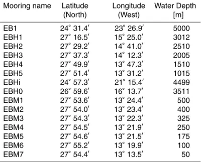
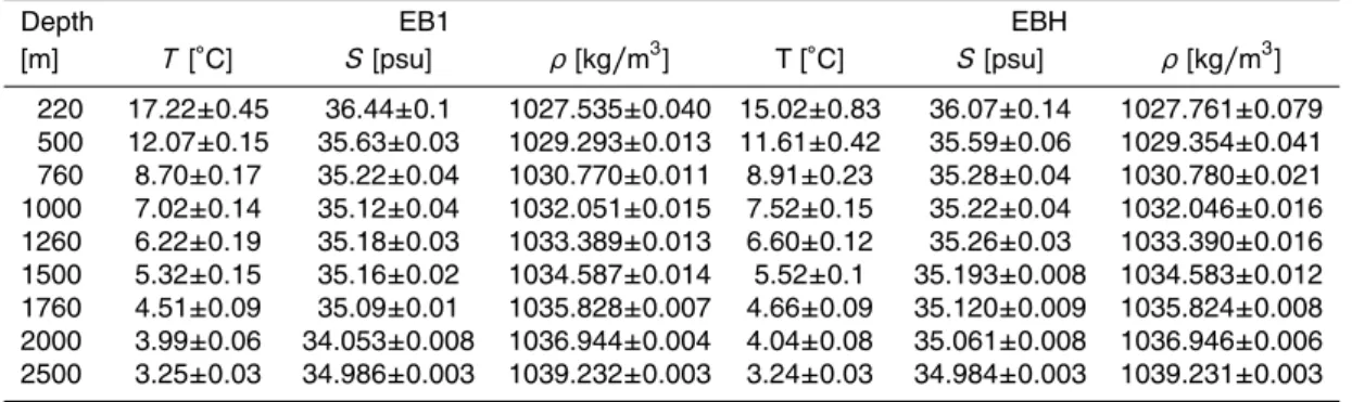
the eastern-boundary (west of Morocco) sub-arrays (Fig. 1). The full-depth moorings have between 11 and 24 CTD sensors at fixed depths throughout the water column; the moorings are serviced at annual intervals (during autumn for the eastern boundary). The western-boundary and eastern-boundary moorings constitute the endpoint density profiles required to calculate the basin-wide zonally integrated geostrophic flow. 5

2.1 The eastern-boundary sub-array

The eastern-boundary sub-array as deployed for the year 2007 is shown in Fig. 2; the nominal positions and water depths of the moorings are given in Table 1. The full water-column mooring EB1 is situated at the base of the continental slope, roughly 1250 km from the coast. The inshore array (EBH) consists of a series of shorter moorings 10

distributed between the African shelf and the base of the eastern continental slope. Each of these “small” moorings covers a certain depth range such that all of them merged together account for the full boundary density profile between the surface and 5000 m.

The periods of the mooring records and the nominal depths of the CTD sensors are 15

given in Tables 2 and 3 for EB1 and EBH, respectively. Vertical sensor spacing in-creases with depth from roughly 100 m near the sea surface, to 200 m at the bottom of the thermocline, to 500 m in the deep ocean. During the different deployment pe-riods the array has been subject to some minor design changes. Initially, from March 2004 to April 2005, EB1 occupied the depth range between 2500 dbar and 4850 dbar. 20

Since April 2005 EB1 has covered the entire water column, with 24 sensors (21 sen-sors between November 2005 and May 2006). The re-deployment of EB1 failed in October 2006, and it was only re-deployed during a cruise in December 2006. For this reason, there is a time gap of ca. 2 months (from 8 October 2006 to 1 December 2006, Table 2). Each of the moorings of the EBH array has between 1 and 6 CTD 25

(7)

OSD

6, 2507–2553, 2009

the AMOC

Title Page

Tables Figures

◭ ◮

Back Close

Full Screen / Esc

profile between 565 dbar and 965 dbar, EBH4 between 1060 dbar to 1460 dbar, EBH3 between 1555 dbar and 1955 dbar, EBH2 at 2060 dbar and EBH1 between 2562 dbar and 2762 dbar. Deep eastern-boundary measurements are taken from EB1 (below roughly 3000 dbar). The same merging procedure applies to the following years. From April 2005, the EBH array had consistently measurements above 500 dbar and two 5

additional moorings (EBH0 and EBHi) were deployed across the slope to account for density measurements in the 3500–4500 dbar pressure range. During the second de-ployment period, all the sensors stopped recording due to battery failures, producing a gap in the data of ca. 3 months (from 2 February 2006 to 22 May 2006, Table 3).

The data recovery on the slope was complicated by mooring losses, most likely 10

due to fisheries activities south of the Canary Islands. For instance, for the period from April 2005 to February 2006, one of the shallower moorings (EBH4) could not be recovered leading to a data loss at the 300–800 dbar pressure range (Rayner et al., 2007). In an attempt to reduce the potential impact of fishing activity, in the deployment during October 2006 the shallowest mooring EBH5 was divided into a set of smaller 15

“mini-moorings”, EBM1 to EBM7, consisting of only one CTD sensor per mooring. However, only two of the “mini-moorings” returned data (EBM4 and EBM1, at 253 dbar and 515 dbar, respectively), two more were recovered with sensors missing (EBM5 and EBM6).

2.2 Data acquisition and processing

20

All the moored sensors discussed here are Seabird SBE37 (MicroCAT), which mea-sure temperature, conductivity and presmea-sure. The sensors acquire data at sampling rates between 15 and 30 min. For calibration, all moored CTD sensors are lowered on a frame together with a reference CTD package (SBE 911) before and after each deployment period. Calibration coefficients for each sensor are computed and linear 25

(8)

OSD

6, 2507–2553, 2009

the AMOC

Title Page

Tables Figures

◭ ◮

Back Close

Full Screen / Esc

Using all the information described in Sect. 2.1, full-depth continuous profiles of tem-perature and salinity and thus of density (ρ) are obtained at each site as follows. Salin-ity is computed and temperature, salinSalin-ity, and pressure are two-day low-pass filtered and interpolated on a half-daily grid. Temperature and salinity are vertically interpo-lated onto a regular 20-dbar pressure grid (Kanzow et al., 2007) using an interpolation 5

technique relying on climatological temperature and salinity gradients between verti-cally adjacent sensor levels (Johns et al., 2005). Finally density (ρ) is computed. For each deployment period, upward integration of temperature and salinity is done up to the uppermost level of measurements available. The only exceptions are for year 2004 and year 2007 at EBH, when the uppermost level of measurements was 540 dbar and 10

240 dbar, respectively, and the data were extrapolated to 120 dbar at each time step as follows. For the year 2004 temperature and salinity are linearly extrapolated to 240 dbar by estimating the gradient from the anomalies at 840 and 540 dbars and then carrying the anomaly at 240 dbar at constant value up to 120 dbar (Kanzow et al., 2007, Supporting Online Material). For the year 2007, the data are linearly extrapolated to 15

120 dbar on the basis of the gradient of the anomaly between the two uppermost levels of measurements.

3 Transport calculations

We start by describing briefly how a time series of strength of the AMOC,ψ_MAX(t), is computed from the observational data (for more details see Kanzow et al., 2009b). 20

Then we show how the contribution of eastern-boundary density variations to the AMOC is calculated.

At 26.5◦N, ψMAX(t) is calculated by the sum of three meridional flow components:

the northward Gulf Stream transport through the Straits of Florida (TGS), the zonally

in-tegrated near-surface Ekman transport (TEK), and the geostrophic mid-ocean transport

25

between the Bahamas and the African coast (TMO). From these transport

(9)

OSD

6, 2507–2553, 2009

the AMOC

Title Page

Tables Figures

◭ ◮

Back Close

Full Screen / Esc

is computed such that

TAMOC(z,t)=TGS(z,t)+TEK(z,t)+TMO(z,t), (1)

wherezdenotes negative depth.

ψMAX(t) at 26.5◦N is defined at each time step as the maximum northward

trans-port in the upper ocean. The northward transtrans-port is integrated downward from the 5

sea surface to the depth levelhmax(t) where the maximum cumulative northward

trans-port is reached at each time step (that is, the depth where the zero crossing between northward and southward flow occurs), according to

ΨMAX(t)=

zZ=0

z=−h_max

TAMOC(z,t)d z. (2)

For the computation ofTAMOC(z,t),TGS(z,t) andTEK(z,t) are computed directly from the

10

cable and wind observations, respectively (Kanzow et al., 2007; Cunningham et al., 2007). T_MO(z,t) has two components: the transport T_WBW(z,t) through the western boundary wedge over the Bahamas continental slope – calculated from direct current meter measurements (Johns et al., 2008) – and the geostrophic transport between the Bahamas and the African coast. The latter is computed from the internal transport, 15

TINT, calculated from the east to west density gradient and a reference transport TC.

TINT is computed by means of the vertical density profiles at the western boundary and

the eastern boundary (ρW andρE), relative to a reference level (href), according to

TINT(z,t)=−(g/ρf)

z Z

z′₌₋_h_ref

[ρE(z′,t)−ρW(z′,t)]d z′,forz >−href, (3)

wheregis the Earth’s gravitational acceleration,ρ is a reference density, andf is the 20

Coriolis parameter. To compute absolute values ofTMO(z,t), a reference transport for

(10)

OSD

6, 2507–2553, 2009

the AMOC

Title Page

Tables Figures

◭ ◮

Back Close

Full Screen / Esc

of no net mass transport across the longitude-depth section at 26.5◦N, which is justified for timescales longer than 10 days (Kanzow et al., 2007). This constraint is equivalent to a perfect compensation among the different flow components, according to

zZ=0

z=−hbot

[TGS(z,t)+TEK(z,t)+TMO(z,t)]d z=0, (4)

wherehbotrepresents the depth of the sea floor.

5

The reference transport of TINT(z,t), namely TC(t), is computed at each time step

according to

TC(t)=−

zZ=0

z=−hbot

[TGS(z,t)+TEK(z,t)+TWBW(z,t)+TINT(z,t)]d z. (5)

The computation ofTCis performed assuming that the compensating meridional

veloc-ity fieldVC(x,z) is spatially uniform (Hirschi et al., 2003) such that

10

TC=VC

zZ=0

z=−h_bot

X_Z_W

X_E

dxd z=VC

zZ=0

z=−h_bot

L(z)d z, (6)

whereXW andXEdenote the position of the western and eastern boundary endpoints,

andLis the effective width of the transatlantic section, which reduces with depth (Kan-zow et al., 2009b).

The absolute mid-ocean transport is then given by 15

TMO(z,t)=TWBW(z,t)+TINT(z,t)+TC(z,t), (7)

withTC(z,t)=VCL(z).

How then is the transport contribution of eastern-boundary densities toψMAX(t)

(11)

OSD

6, 2507–2553, 2009

the AMOC

Title Page

Tables Figures

◭ ◮

Back Close

Full Screen / Esc

time-variable contribution comes from eastern-boundary densities. As there is no sig-nificant correlation between density fluctuations at the western boundary (offthe Ba-hamas) and the eastern boundary for annual and higher frequencies (Kanzow et al., 2009b), we can isolate the eastern-boundary contribution to TMO(z,t) by prescribing

a time-invariant density profile at the western boundary at each time step in Eq. (3). 5

We use

T_INTEB(z,t)=−(g/ρf) z Z

z′₌₋_h_ref

[ρE(z′,t)−ρW(z′)]d z′,for −href< z <−hup, (8)

where the overbar denotes the time-average. The reference depth,h_ref, is taken as the greatest common depth of the moorings in the east (4900 m), andhup represents the

uppermost measurement level at the eastern boundary;hup differs between the diff

er-10

ent mooring deployment periods (Tables 2 and 3). To obtain estimates for the entire water column, the profiles of transport per unit depth resulting from Eq. (8) are linearly extrapolated from the uppermost measurement level to the surface for each time step, on the basis of the gradient of the transport anomaly between the two uppermost levels of measurements. When required, the profiles are linearly interpolated in time to fill the 15

time gaps of 1–2 weeks between mooring recovery and redeployment.

We then add at each time step the resulting transport per unit depth anomaly profiles arising from Eq. (8) to the time-mean contribution of all the other components according to

T_AMOCEB (z,t)=T¯GS(z)+T¯EK(z)+T¯WBW(z)+T_INTEB(z,t)+T_CEB, (9)

20

such that the compensating transport at each time stepT_CEB(t) is given by

T_CEB(t)=−

zZ=0

z=−h_bot

(12)

OSD

6, 2507–2553, 2009

the AMOC

Title Page

Tables Figures

◭ ◮

Back Close

Full Screen / Esc

Consistent with Eq. (2), the eastern-boundary density contribution to the strength of the AMOC is computed from

ΨEB_MAX(t)=

zZ=0

z=−h_{max eb}

T_AMOCEB (z,t)d z, (11)

wherehmax eb(t) is the depth where the zero crossing between northward and

south-ward flow occurs at each time step forT_AMOCEB (z,t).

5

As motivated in Sect. 1,ΨEBMAX(t) is computed using the densities observed at either

EB1 or EBH. The profiles of transport per unit depth computed according to Eq. (9) using EB1 and EBH will be referred to asT_AMOCEB1 andT_AMOCEBH , respectively. The eastern-boundary density contributions to the AMOC computed from Eq. (11) will be referred to asΨEB1MAXandΨ

EBH

MAX, respectively.

10

4 Eastern-boundary hydrographic characteristics

Next we examine the hydrographic properties of the water masses observed at EB1 and EBH to explore whether the temporal fluctuations of the properties between the two sites are coherent. For this, we examine temporal anomalies. Both data sets cover the period from 4 March 2004 to 14 October 2007 (ca. 3.5 years of data). Notice that for 15

clearer visualization, we plot and discuss temporal anomalies relative to the time mean of each separate deployment period (Figs. 3–6). In all calculations based on density anomalies, however, we compute temporal anomalies relative to the time mean of the entire 3.5 years unless explicitly noted. Throughout this study fluctuations are reported in±one standard deviation.

20

(13)

OSD

6, 2507–2553, 2009

the AMOC

Title Page

Tables Figures

◭ ◮

Back Close

Full Screen / Esc

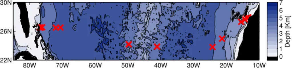
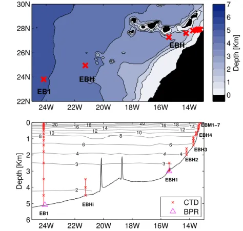
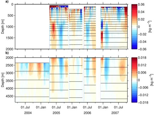
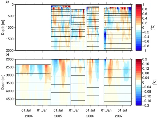
the major density and temperature anomalies are of uniform sign between the bottom and at least ca. 800 m, with the exception of the event in December 2006 (see below, Figs. 3 and 4). Maximum mid-depth density anomalies are found near 1000 m over the whole period; we observe the most intense density anomalies during May 2005, August 2005, July 2006, December 2006, and February 2007. The positive density anomaly 5

event with a maximum by the end of May 2005 at 1000 m lasts for 10 weeks, with the more intense anomalies (exceeding 0.02 kg/m3) confined to a layer between 800 and 1500 m. This density event is associated with positive temperature and salinity anoma-lies of up to 0.35◦C and 0.1 psu, respectively, but the latter have their maximum at ca. 800 m, while at the depth of the maximum density anomaly (ca. 1000 m) temperature 10

and salinity anomalies of only−0.1◦C and 0.03 psu are found. This implies that salin-ity dominates this denssalin-ity excursion near its maximum. There are three major events of anomalously negative density, all with similar characteristics, taking their extreme values at the end of August 2005, at the beginning of July 2006, and at mid-February 2007, respectively, and lasting for 5–6 weeks, 3 weeks, and 5 weeks, respectively. 15

Negative density anomalies during the three events exceed 0.02 kg/m3 at the depth interval between ca. 900 and 1500 m. During the August 2005 and July 2006 events, density minima occur at a deeper level than the corresponding salinity and temperature extrema. During December 2006, quite a different density anomaly can be identified, with two cores of opposite sign, negative in the range 600–1200 m and positive in the 20

range 1200–2000 m. This event lasts for ca. 3 weeks, and the strongest anomalies are found at the end of December 2006, with temperature dominating the density anomaly (Figs. 3a and 4a).

Some of these features seem to be water mass anomalies associated with local small-scale eddy circulations, rather than just temperature/salinity variations due to 25

(14)

OSD

6, 2507–2553, 2009

the AMOC

Title Page

Tables Figures

◭ ◮

Back Close

Full Screen / Esc

meaning cyclonic circulation) passing by the mooring. For instance, for the positive density event on May 2005 described above (Fig. 3a), we observe that the core of the temperature (Fig. 4a) and salinity (not shown) anomalies (ca. 800 m) offset from the core of the density anomaly (ca. 1000 m) (Fig. 3a), suggesting that this is a salty anti-lens passing by the mooring.

5

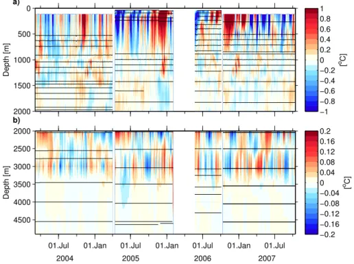
Along the EBH array, the strongest density anomalies (exceeding±0.1 kg/m3) are found in the upper 500 m (Fig. 5a), occasionally extending further down in the water column to up to 1400 m. Above 500 m, positive density anomalies that are persistent over longer periods (3–7 weeks) occur during April–May 2004, April–May 2005 and May 2007, while negative density anomalies that are persistent over longer periods 10

(5–7 weeks) occur during October–November 2004, November–December 2005 and October–November 2006. The density anomalies in the upper ocean are dominated by temperature changes (Fig. 6a). In December 2005, pronounced mid-depth maximum positive density anomalies of 0.04 kg/m3are found at 1300 m (Fig. 5a); they are asso-ciated with pronounced temperature and salinity anomalies of respectively 0.7◦C and 15

0.2 psu at the same depth level (Fig. 6a). The anomalous warm salty water occurs at depths that are expected for mixing with Mediterranean water coming out of the Strait of Gibraltar at 36◦N.

The vertical scales of the in-situ density anomalies at EB1 and EBH show pro-nounced differences (Figs. 3 and 5). At EB1, density anomalies extend much deeper, 20

throughout almost the entire water column, while at EBH the density anomalies are stronger than at EB1 but they mainly occur in the upper 1400 m. The time scales of the anomalies are also different between EB1 and EBH. At EB1 the variability is dominated by long periods of a several weeks to several months, while at EBH density anomalies exhibit pronounced short-periodic variability with dominant periods around 13 days, 25

(15)

OSD

6, 2507–2553, 2009

the AMOC

Title Page

Tables Figures

◭ ◮

Back Close

Full Screen / Esc

out fortnightly tidal forcing, and so their origin is unclear at present. This large verti-cal coherence gives us confidence in the sampling strategy at EBH, confirming that the variability is well captured by the “merging” of the moorings distributed across the continental slope.

The temporal standard deviations of temperature, salinity and in-situ density at EB1 5

and EBH computed for the period between 13 April 2005 and 14 October 2007 (when both moorings have full-depth measurements) are shown in Fig. 8. Both EB1 and EBH display the most pronounced differences in rms variability in temperature, salinity and density between 220 m and 800 m (Fig. 8, Table 4). Amplitudes at EB1 are smaller than those at EBH above 800 m. At both sites, the largest variability is found in the 10

uppermost level of measurements (220 m at EB1 and 120 m at EBH). At 220 m, vari-ability in temperature, salinity, and density at EB1 is smaller than that at EBH by 0.38◦C, 0.04 psu, and 0.04 kg/m3, respectively. In particular, at 220 m rms density fluctuations are±0.04 kg/m3at EB1 and±0.08 kg/m3at EBH (Fig. 8c). Temperature at EB1 ex-hibits maximum variability of±0.45◦C at the surface, with a local minimum of 0.15◦C at 15

ca. 900 m, and a local maximum of 0.2◦C at ca. 1300 m. Temperature and salinity at EBH display maximum variability of±0.95◦C and±0.16 psu respectively at the surface (120 m). At mid-depths, maximum variability differences between EB1 and EBH are found at ca. 1300 m, where temperature and salinity variability at EB1 exceeds that at EBH, as a result of the deep-reaching anomalies shown in Figs. 3 and 4. However, 20

there is no difference in density variability between EB1 and EBH at this depth level, indicating that even though temperature and salinity vary more at EB1, their variations are density-compensated such that there is no stronger signal in density at EB1. At both sites, the vertical distribution of rms variability in temperature is similar to that in salinity, with both properties fluctuating in-phase (Fig. 8a and b).

(16)

OSD

6, 2507–2553, 2009

the AMOC

Title Page

Tables Figures

◭ ◮

Back Close

Full Screen / Esc

5 Transport variability

We now investigate how the differences between the density fluctuations at EB1 and EBH impact the estimates of basin-wide integrated transports. Unless otherwise noted, all the transport time series discussed here are 10-day low-pass filtered, in order to keep valid the assumption of transport compensation required for the computation of 5

ψMAX(t) (Kanzow et al., 2007). Results for EB1 are shown only after April 2005, when

measurements at EB1 covered the entire water column. A major difference between EB1 and EBH is that T_AMOCEB1 (Fig. 9) contains less energy at daily to weekly periods than doesT_AMOCEBH (Fig. 10), consistent with the density observations (Figs. 3 and 5). BothT_AMOCEB1 and T_AMOCEBH exhibit stronger fluctuations in the upper layer (above 1400 m 10

forT_AMOCEB1 and above 1000 m forT_AMOCEBH ) compared to the deeper layer. Below roughly 1500 m the fluctuations ofT_AMOCEB1 tend to be stronger than those ofT_AMOCEBH . The vertical structure of the profiles is dominated by a first mode-like structure, as there is mostly one zero crossing over the record that is at a constant depth. However, there are exceptions to this pattern, when the vertical structure is more complex and displays two 15

zero crossings. This occurs only during short periods, for instance from the beginning of July to the end of August 2007 forT_AMOCEB1 (Fig. 9), and from the beginning of August 2007 to the end of September 2007 forT_AMOCEBH (Fig. 10).

The first empirical orthogonal function (EOF) modes both of the anomalies about a time-mean vertical profile ofT_AMOCEB1 and ofT_AMOCEBH account for roughly 80% of the vari-20

ance each, and both have large vertical shear in the upper ocean (Fig. 11). A closer look reveals, however, that the first modes ofT_AMOCEB1 andT_AMOCEBH are very different. The zero crossing of the first EOF mode occurs 700 m deeper forT_AMOCEB1 (1740 m) than for

T_AMOCEBH (1076 m), in agreement with the deep-reaching density anomalies observed at EB1 (Fig. 3). The first EOF mode ofT_AMOCEB1 shows two regions of strong shear above 25

(17)

OSD

6, 2507–2553, 2009

the AMOC

Title Page

Tables Figures

◭ ◮

Back Close

Full Screen / Esc

a region of weak shear. In contrast, the first mode ofT_AMOCEBH has strong but monoton-ically decreasing shear between the surface and 1300 m, below its zero crossing at 1000 m; at 1300 m the shear drops abruptly. In the deep ocean, bothT_AMOCEB1 andT_AMOCEBH

exhibit less shear compared to the upper ocean, butT_AMOCEB1 has more shear thanT_AMOCEBH . Below roughly 2870 m the amplitude of the first EOF mode ofT_AMOCEB1 is larger than for 5

T_AMOCEBH . As with the first mode, the second EOF mode of T_AMOCEB1 (accounting for 14% of the variance) has deeper zero crossings and more shear in the deep ocean com-pared to the second EOF mode ofT_AMOCEBH (accounting for 15% of the variance). These differences in vertical structure suggest that the dynamics governing the transport fluc-tuations are different at EB1 and EBH. Note that the vertical structures of the leading 10

EOF modes of T_AMOCEB1 and T_AMOCEBH show no obvious relationship to the vertical water mass structure. Notice also that despite the differences between the EOF modes, the depths of the zero crossings between northward and southward flow are very similar forT_AMOCEB1 andT_AMOCEBH , occurring on average at 1073 m (±44 m) forT_AMOCEB1 and at 1080 m (±40 m) forT_AMOCEBH .

15

We now focus on the fluctuations about the time mean of the overturning trans-port defined according to Eq. (11) using EB1 and EBH (ΨEB1MAX and Ψ

EBH

MAX, Fig. 12).

The maximum anomaly of ΨEB1MAX is 4.7 Sv on 29 August 2005, corresponding to the

strongest negative density anomaly event (Fig. 3), while the minimum anomaly is−4 Sv on 29 May 2005, corresponding to the strongest positive density anomaly event (Fig. 3). 20

This yields a maximum transport range of almost 9 Sv inΨEB1MAX. The maximum anomaly

ofΨEBHMAXis 5.9 Sv on 14 October 2007, and the minimum anomaly is−6.3 Sv on 3 April

2007, giving a transport range of 12.2 Sv inΨEBHMAX. The 30-month record of the

fluc-tuations of ΨEB1MAX has a standard deviation of ±1.7 Sv, and the 42 month record of ΨEBHMAX has a standard deviation of ±2 Sv (Fig. 12). The integral time scale, obtained

25

by integrating the autocorrelation function out to the first zero-crossing, is 24 days for

ΨEB1MAXand 22 days forΨ EBH

(18)

OSD

6, 2507–2553, 2009

the AMOC

Title Page

Tables Figures

◭ ◮

Back Close

Full Screen / Esc

ofΨEB1MAX and 62 dof in our (longer) time series ofΨ EBH

MAX. Thus, there are 15 and 18

effectively independent measurements per year for ΨEB1MAX and Ψ EBH

MAX, respectively. If

we assume measurement errors negligible, we could resolve year-to-year changes of 0.6 Sv ([(1.72/15∗2)]1/2) forΨEB1MAXand 0.6Sv([(1.9

2

/18∗2)]1/2)forΨEBHMAX.

Although the variability of ΨEB1MAX and Ψ EBH

MAX differs by only 0.3 Sv in rms, their

fre-5

quency distribution displays markedly different characteristics (Fig. 13). Both ΨEB1MAX

and ΨEBHMAX have dominant variance at low frequencies, and for periods longer than

50 days the spectra of the two time series are not significantly different. However, for periods shorter than 50 days, the variance ofΨEB1MAX drops rapidly, such that for

peri-ods between 10 and 50 days the variance ofΨEB1MAXis a factor of 10 smaller than that of

10

ΨEBHMAX. Of the spectral peaks inΨ EBH

MAX, only the one around 13 days is clearly significant

at the 95% confidence level; this peak is associated with the 13-day density variations that are coherent down to 3500 m (Sect. 4, Fig. 7). A cross-correlogram of 50-day low-pass filtered time series ofΨEB1MAX andΨ

EBH

MAX fails to show significant correlation at any

time lag between the two time series at the 95% confidence level (not shown), implying 15

that we cannot identify potential westward signal propagation between the two sites through long Rossby waves.

The results presented here show that there is little agreement between the transports estimates from EB1 and EBH. There are considerable differences between EB1 and EBH in terms of amplitude, vertical structure and frequency distribution of the resulting 20

mid-ocean geostrophic transport fluctuations. This implies that density fluctuations at the eastern boundary of the 26.5◦N section need to be monitored across the continen-tal slope. Mechanisms that are unrelated to the AMOC (such as basin-interior eddies) appear to influence strongly the density variability at EB1 on the time scales under consideration. In addition, the tall mooring EB1 is too far offshore to detect potential 25

(19)

OSD

6, 2507–2553, 2009

the AMOC

Title Page

Tables Figures

◭ ◮

Back Close

Full Screen / Esc

of the paper will therefore rely entirely on EBH.

6 Seasonal variability

We now investigate the seasonal cycle in the density anomalies. Given that the obser-vations span 42 months, the seasonal cycle represents the longest period that we can analyze with confidence. The monthly averages of in-situ density at selected depths 5

levels (Fig. 14) show that there is a pronounced seasonal variability in density right at the continental slope offnorthwest Africa at 26.5◦N. Maximum values occur during spring (April/May) and minimum values during autumn (October/November). The sea-sonal cycle is coherent throughout the upper ocean and is surprisingly deep-reaching as it can be observed up to a depth of 1400 m. For all depth levels between 100– 10

1400 m, the seasonal cycle is statistically significant.

As a result of the deep reaching seasonal cycle in density, there is also a pronounced seasonal cycle in the eastern-boundary contribution to the AMOC, as monthly means of the anomalies ofΨEBHMAXshow (Fig. 15). The observed seasonal density changes drive

an enhanced southward upper mid-ocean flow in spring (April), resulting in a minimum 15

in theΨEBHMAX, and vice-versa in autumn (October). The amplitude of the seasonal cycle

ofΨEBHMAX is 5.2 Sv peak-to-peak, with the peak in April being statistically different from

the peak in October.

7 Discussion

The largest density anomalies at the eastern-boundary continental slope (EBH) at 20

(20)

OSD

6, 2507–2553, 2009

the AMOC

Title Page

Tables Figures

◭ ◮

Back Close

Full Screen / Esc

at this period. It can be expected that this phenomenon is associated with sea surface height anomalies; therefore a possible way to investigate the spatial scales associated with the 13-day period might be via satellite altimeter data. However, aliasing due to the insufficient temporal resolution (the Jason altimeter has a repeat cycle of 10 days) will make such an analysis problematic. The closeness of the 13-day fluctuations to the 5

fortnightly tidal periods could point to a tidal origin of this signal. However, fortnightly tidal fits applied to the EBH densities give rather different results for different depth lev-els (not shown), suggesting that the 13-day fluctuations are not regular enough to be tidal oscillations. Alternatively, the geometry of the semi-enclosed basin south of the Canary Island where we take our measurements might play a role in the generation of 10

13-day basin modes excited by stochastic wind forcing.

The temporal variability and the vertical structure of the transports derived from EB1 and EBH have different characteristics. The transports derived from EB1 show much less energy at periods shorter than 50 days, compared to the transports derived from EBH. The leading EOF transport modes show that the vertical shear of the transport 15

arising from EB1 and EBH is especially different in the upper 1000 m. This points to different dynamics governing the density fluctuations at EB1 and EBH. Kanzow et al. (2009b) show that the local wind forcing is very different, and much weaker, at EB1 than EBH. Hence, local coastal wind forcing appears to play an important role in setting the variability at EBH. At EB1, the deep-reaching density anomalies may be 20

linked to mesoscale eddies associated with the open ocean circulation. Contrary to the original planning (Marotzke et al., 2002), measurements at EB1 and EBH cannot serve as a backup for each other: densities need to be measured right at the continental slope to compute the eastern boundary density contribution to the AMOC.

Lee and Marotzke (1998) had proposed a decomposition of the meridional over-25

(21)

OSD

6, 2507–2553, 2009

the AMOC

Title Page

Tables Figures

◭ ◮

Back Close

Full Screen / Esc

the eastern boundary contribution to the shear component is covered by the density measurements. But how about the external mode? Hirschi and Marotzke (2007) found in an eddy-permitting model of the Atlantic that the external mode mostly affected the time mean flow but not the temporal variability. They noticed that the external mode contribution to the AMOC becomes sizeable for large bottom velocities. For small bot-5

tom velocities the strength and vertical structure of the simulated AMOC (including the external mode) could be reconstructed reliably from eastern and western boundary densities as we attempted in this study. At 26.5◦N (if at all) we expect the external mode to be relevant in the western boundary current system where large bottom veloc-ities both in upper ocean (Antilles Current) and the deep western boundary current can 10

occur (Johns et al., 2008). The direct current meter measurements across the western boundary continental slope are used to capture this contribution. At the eastern bound-ary at 26.5◦N bottom velocities are much smaller and therefore our reconstruction of the AMOC from densities at the eastern boundary is unlikely to be affected significantly by a possible misrepresentation of external mode.

15

The 10-day low-pass filtered 42-month long record of the eastern boundary contribu-tion to the AMOC at 26.5◦N, ΨEBHMAX, has a temporal standard deviation of±2 Sv.

Kan-zow et al. (2009b) show that the overall AMOC variability is±4.9 Sv and that the west-ern boundary contribution of the mid-ocean section to the AMOC varies by ±2.3 Sv. The latter indicates that the western and eastern boundaries of the mid-ocean section 20

contribute to the AMOC variability by roughly the same amount. This result contradicts earlier findings by Longworth (2007), who found from historical CTD measurements that the eastern boundary contribution was only half of that from the western bound-ary. However, the total western-boundary transport contribution to the AMOC also includes variability of the Gulf Stream and is hence significantly larger than that from 25

the eastern boundary.

(22)

south-OSD

6, 2507–2553, 2009

the AMOC

Title Page

Tables Figures

◭ ◮

Back Close

Full Screen / Esc

ward upper mid-ocean flow in spring, implying maximum reduction of the AMOC, and anomalous northward upper mid-ocean flow in autumn, implying maximum strength-ening of the AMOC. The eastern boundary causes a peak-to-peak seasonal cycle of the AMOC of 5.2 Sv, clearly dominating the peak-to-peak seasonal cycle of thetotal AMOC of 7.0 Sv (Kanzow et al., 2009b). This dominant influence is surprising and 5

arises because western boundary transports do not display such a clear seasonal cy-cle when isolated in a similar fashion.

A detailed analysis of the mechanisms driving the seasonal density fluctuations is subject of ongoing work and is beyond the scope of this paper. We do, however, offer a preliminary analysis here. Several authors reported seasonal anomalies of the east-10

ern boundary current system offNorthwest Africa based on mooring-based measure-ments and hydrographic observations. A strong northward current during autumn close to the African shelf in the 1300 m deep channel between Lanzarote and Africa at 29◦N was observed (Knoll et al., 2002; Hern ´andez-Guerra et al., 2003). Knoll et al. (2002) found maximum southward flow in the upper 200 m in the middle of the channel be-15

tween Lanzarote and Africa during spring. The seasonal northward transport in the Canary Current system is consistent with the anomalous northward transports (and minimum in in-situ density) we find in October (Fig. 15). The phase of maximum ward flow during spring reported by Knoll et al. (2002) is consistent with the south-ward transports (and maximum in in-situ density) we find in April (Fig. 15). This sug-20

gests a link with the variability we find inΨEBHMAXbut further analysis needs to be done

on the variability of the eastern boundary current. A possible way to investigate this would be to compare the available current-meter time series at the Lanzarote passage (Hern ´andez-Guerra et al., 2003) with our observations of ΨEBHMAX. If good agreement

is found, this would allow expanding the eastern-boundary AMOC time series back 25

(23)

OSD

6, 2507–2553, 2009

the AMOC

Title Page

Tables Figures

◭ ◮

Back Close

Full Screen / Esc

The Moroccan coastal upwelling undergoes seasonal changes induced by the coast-parallel trade winds. The band between 25◦N and 43◦N along the African coast ex-hibits strongest coastal upwelling during summer and autumn (e.g., Wooster et al., 1975; Mittelstaedt et al., 1983). We observe maximum densities in April/May, two months earlier than the maximum upwelling occurs. Also coastal upwelling is thought 5

to bring waters from 200 or 300 m depth to the surface. In contrast, our analysis sug-gests coherent seasonal density changes down to 1400 m. For these reasons coastal upwelling is unlikely to be the direct driver of the seasonal density and transport cy-cles. Instead, the vertical structure suggests a first baroclinic mode as a result of the displacement of the density surfaces induced by the wind stress curl. A preliminary 10

analysis of the Quikscat-based SCOW (Scatterometer Climatology of Ocean Winds) seasonal wind stress curl climatology (Risien and Chelton, 2008) reveals a pronounced seasonal cycle in eastern boundary wind stress curl, which leads the density anomaly by roughly 90 degrees or 3 months (Fig. 16). The out-of-phase relationship is plau-sible, as uplifting of the density surfaces should prevail during the winter phases of 15

enhanced cyclonic wind curl anomalies. Therefore maximum positive density anoma-lies can be expected in spring, when the transition from cyclonic to anti-cyclonic wind stress curl anomalies takes place. The summer period of anti-cyclonic wind stress curl then should lead to the observed maximum negative density anomalies in autumn as a result of the maximum depression of the density surfaces. The SCOW data set ex-20

hibits limitations in resolving the wind curl near the coast close to the mooring locations and needs to be further investigated.

8 Conclusions

Based on 3.5 years of moored temperature and salinity data at the eastern boundary of the Atlantic at 26.5◦N from a tall mooring (EB1) located at the base of the continental 25

(24)

OSD

6, 2507–2553, 2009

the AMOC

Title Page

Tables Figures

◭ ◮

Back Close

Full Screen / Esc

– Density anomalies at EBH are often coherent down to 1400 m; 13-day density fluctuations even reach down to 3500 m. This vertical coherence confirms the validity of the sampling strategy at EBH, including the merging of the profiles.

– There are significant transports between EB1 and EBH, so contrary to the original planning, measurements at EB1 cannot serve as backup for EBH. Density needs 5

to be observed right at the continental slope as part of an AMOC monitoring strategy.

– Eastern-boundary density variations contribute±2 Sv rms AMOC variability, sim-ilar to the contribution from the western boundary (east of the Bahamas) to the mid-ocean geostrophic component of the AMOC.

10

– The seasonal cycle in density at the eastern boundary is coherent between 100 m and 1400 m, with maximum positive and negative density anomalies in spring and autumn, respectively. Resulting is a minimum AMOC in spring and a maximum AMOC in autumn, with a peak-to-peak amplitude of the seasonal cycle of 5.2 Sv caused by the eastern boundary, which dominates the 7.0 Sv seasonal cycle of 15

the total AMOC.

Acknowledgements. We thank the captains and crews of the research vesselsDiscovery and

Poseidon, and the UKORS mooring team. The mooring operations have been funded by NERC RAPID. This work was supported by the Max Planck Society and the International Max Planck Research School on Earth System Modelling.

20

The service charges for this open access publication have been covered by the Max Planck Society.

References

Baringer, M. O. and Larsen, J. C.: Sixteen years of Florida Current Transport at 27◦N, Geophys. 25

(25)

OSD

6, 2507–2553, 2009

the AMOC

Title Page

Tables Figures

◭ ◮

Back Close

Full Screen / Esc

Interactive Discussion Beckmann, A.: Vertical structure of midlatitude mesoscale instabilities, J. Phys. Oceanogr., 18,

1354–1371, 1988.

Bryden, H. L., Longworth, H. R., and Cunningham, S. A.: Slowing of the Atlantic meridional overturning circulation at 25 N, Nature, 438, 655–657, doi:10.1038/nature04385, 2005. Cunningham, S. A., Kanzow, T., Rayner, D., Baringer, M. O., Johns, W. E., Marotzke, J., Long-5

worth, H. R., Grant, E. M., Hirschi, J. J.-M., Beal, L. M., Meinen, C. S., and Bryden, H. L.: Temporal variability of the Atlantic meridional overturning circulation at 26.5◦N, Science, 317, 935–938, 2007.

Hern ández-Guerra, A., Fraile-Nuez, E., Borges, R., L ópez-Laatzen, F., V éllez-Belchi, P., Par-rilla, G., and M üller, T.: Transport variability in the Lanzarote passage (eastern boundary 10

current of the North Atlantic Subtropical Gyre), Deep-Sea Res. I, 50, 189–200, 2003. Hall, M. M. and Bryden, H. L.: Direct estimates and mechanisms of ocean heat transport,

Deep-Sea Res., 29(3A), 339–359, 1982.

Hirschi, J., Baehr, J., Marotzke, J., Stark, J., Cunningham, S., and Beismann, J. O.: A moni-toring design for the Atlantic meridional overturning circulation, Geophys. Res. Lett., 30(7), 15

1413, doi:10.1029/2002GL016776, 2003.

Hirschi J. J.-M. and Marotzke, J.: Reconstructing the meridional overturning circulation from boundary densities and the zonal wind stress, J. Phys. Oceanogr., 37(3), 743–763, 2007. Johnson, H. L. and Marshall, D. P.: Localization of abrupt change in the North Atlantic

thermo-haline circulation, Geophys. Res. Lett., 29(6), 1083, doi:10.1029/2001GL014140, 2002. 20

Johnson, H. L. and Marshall, D. P.: Global teleconnections of meridional overturning circulation anomalies, J. Phys. Oceanogr., 34, 1702–1722, 2004.

Johns, W. E., Kanzow, T., and Zantopp, R.: Estimating ocean transports with dynamic height moorings: An application in the Atlantic deep western boundary current, Deep-Sea Res. I, 52, 1542–1567, 2005.

25

Johns, W. E., Beal, L. M., Baringer, M. O., Molina, J., Cunningham, S. A., Kanzow, T., and Rayner, D.: Variability of shallow and deep western boundary currents off the Bahamas during 2004–2005: First results from the 26◦N RAPID-MOC array, J. Phys. Oceanogr., 38, 605–623, 2008.

Kawase, M.: Establishment of mass-driven abyssal circulation, J. Phys. Oceanogr., 17, 2294– 30

2317, 1987.

(26)

OSD

6, 2507–2553, 2009

the AMOC

Title Page

Tables Figures

◭ ◮

Back Close

Full Screen / Esc

Interactive Discussion Deep-Sea Res. I, 53, 528–546, 2006.

Kanzow, T., Cunningham, S. A., Rayner, D., Hirschi, J. J.-M., Johns, W. E., Baringer, M. O., Bryden, H. L., Beal, L. M., Meinen, C. S., and Marotzke, J.: Observed flow compensation associated with the MOC at 26.5◦N in the Atlantic, Science, 317, 938–941, 2007.

Kanzow, T., Hirschi, J. J.-M., Meinen, C. S., Rayner, D., Cunningham, S. A., Marotzke, J., 5

Johns, W. E., Bryden, H. L., Beal, L. M., and Baringer, M. O.: A prototype system for observ-ing the Atlantic Meridional Overturnobserv-ing Circulation – scientific basis, measurement and risk mitigation strategies, and first results, J. Operat. Oceanogr., 1, 19–28, 2008.

Kanzow, T., Johnson, H., Marshall, D., Cunningham, S. A., Hirschi, J. J.-M., Mujahid, A., Bry-den, H. L., and Johns, W. E.: Basin-wide integrated volume transports in an eddy-filled 10

ocean, J. Phys. Oceanogr., doi:10.1175/2009JPO4185.1 in press, 2009a.

Kanzow, T., Cunningham, S. A., Johns, W. E., Hirschi, J. J.-M., Marotzke, J., Baringer, M. O., Meinen, C. S., Chidichimo, M. P., Atkinson, C., Beal, L. M., Bryden, H. L., and Collins, J.: Seasonal variability of the Atlantic meridional overturning circulation at 26.5◦N, J. Climate, submitted, 2009b.

15

Knoll, M., Hern ández-Guerra, A., Lenz, B., L ópez-Laatzen, F., Mach´ın, F., M üller, T. J., and Siedler, G.: The Eastern Boundary Current System between the Canary islands and the African coast, Deep-Sea Res. II, 49(17), 3427–3440, 2002.

K ¨ohl, A.: Anomalies of meridional overturning: Mechanisms in the North Atlantic, J. Phys. Oceanogr., 35, 1455–1472, 2005.

20

Larsen, J. C.: Transport and heat flux of the Florida Current at 27◦N derived from cross-stream voltages and profiling data: theory and observations, Philos. T. Roy. Soc. London, A 338, 169–236, 1992.

Lee, T. and Marotzke, J.: Seasonal cycles of meridional overturning and heat transport of the Indian Ocean, J. Phys. Oceanogr., 28, 923–943, 1998.

25

Longworth, H. R.: Constraining variability of the Atlantic meridional overturning circulation at 26.5◦N from historical observations, Ph.D. Thesis, School of Ocean and Earth Science, University of Southampton, Southampton, UK, 198 pp, 2007.

Marotzke, J., Cunningham, S. A., and Bryden, H. L.: Monitoring the Atlantic meridional over-turning circulation at 26.5◦N, Proposal accepted by the Natural Environment Research Coun-30

cil (UK), online available at: http://www.noc.soton.ac.uk/rapidmoc/, 2002.

(27)

OSD

6, 2507–2553, 2009

the AMOC

Title Page

Tables Figures

◭ ◮

Back Close

Full Screen / Esc

Interactive Discussion Percival, D. B. and Walden, A. T.: Spectral Analysis for Physical Applications: Multitaper and

Conventional Univariate Techniques, Cambridge University Press, Cambridge, UK, 583 pp., 1993.

Rayner, D. (Ed.): RV Ronald H. Brown Cruise RB0602 and RRS Discovery Cruise D304, Rapid Mooring Cruise March and May 2006, National Oceanography Centre Southampton, Cruise 5

report No. 16, Southampton, UK, 165 pp., 2007.

Risien, C. M. and Chelton, D. B.: A global climatology of surface wind and wind stress fields from eight years of QuikSCAT scatterometer data, J. Phys. Oceanogr., 38, 2379–2413, 2008. Roemmich, D. and Wunsch, C.: Two transatlantic sections: Meridional circulation and heat flux

in the subtropical North Atlantic Ocean, Deep-Sea Res., 32(6), 619–664, 1985. 10

Wooster, W. S., Bakun, A., and McLain, D. R.: The seasonal upwelling cycle along the eastern boundary of the North Atlantic, J. Mar. Res., 34, 131–141, 1976.

(28)

OSD

6, 2507–2553, 2009

the AMOC

Title Page

Tables Figures

◭ ◮

Back Close

Full Screen / Esc

Table 1.Nominal positions and water depths of eastern-boundary moorings.

Mooring name Latitude Longitude Water Depth

(North) (West) [m]

EB1 24◦31.4′ 23◦ 26.9′ 5000

EBH1 27◦16.5′ 15◦25.0′ 3012

EBH2 27◦29.2′ 14◦41.0′ 2510

EBH3 27◦37.3′ 14◦12.3′ 2005

EBH4 27◦49.9′ 13◦47.3′ 1510

EBH5 27◦51.4′ 13◦31.2′ 1015

EBHi 24◦57.3′ 21◦ 15.4′ 4499

EBH0 26◦59.6′ 16◦13.7′ 3511

EBM1 27◦53.6′ 13◦24.4′ 500

EBM2 27◦54.0′ 13◦23.4′ 400

EBM3 27◦54.3′ 13◦22.3′ 325

EBM4 27◦54.5′ 13◦21.9′ 250

EBM5 27◦54.6′ 13◦21.5′ 175

EBM6 27◦55.2′ 13◦19.9′ 100

(29)

OSD

6, 2507–2553, 2009

the AMOC

Title Page

Tables Figures

◭ ◮

Back Close

Full Screen / Esc

Table 2.Periods of mooring records and nominal pressure levels of sensors of EB1 mooring.

Start Date End Date Nominal Instrument Pressures [dbar] T/S Levels

04 Mar 04 07 Apr 05 2500, 3000, 3500, 4000, 4500, 4850 6

13 Apr 05 18 Nov 05 94, 144, 219, 294, 369, 444, 544, 644, 744, 844, 944, 1044, 1144, 1244, 1444, 1644, 1844, 2044, 2544, 3044, 3544, 4044, 4544, 4894

24

28 Nov 05 03 May 06 250, 325, 400, 500, 600, 700, 800, 900, 1000, 1100, 1200, 1400, 1600, 1800, 2000, 2500, 3000, 3500, 4000, 4500, 4850

21

22 May 06 08 Oct 06 110, 160, 250, 325, 400, 475, 550, 650, 750, 850, 950, 1050, 1150, 1250, 1450, 1550, 1750, 1950, 2150, 2650, 3150, 3650, 4150, 4800

24

01 Dec 06 14 Oct 07 50, 100, 175, 250, 325, 400, 500, 600, 700, 800, 900, 1000, 1100, 1200, 1400, 1600, 1800, 2000, 2500, 3000, 3500, 4000, 4500, 4850

(30)

OSD

6, 2507–2553, 2009

the AMOC

Title Page

Tables Figures

◭ ◮

Back Close

Full Screen / Esc

Table 3.Periods of mooring records and nominal pressure levels of sensors of EBH array.

Start Date End Date Nominal Instrument Pressures [dbar] T/S Levels

04 Mar 04 01 Apr 05 565, 665, 765, 915, 965 (EBH5); 1060, 1160, 1260, 1410, 1460 (EBH4); 1555, 1655, 1755, 1905, 1955 (EBH3); 2060 (EBH2); 2562, 2762 (EBH1)

18

13 Apr 05 02 Feb 06 50, 100, 175, 250 (EBH5)b; 240, 315, 415, 515, 615, 715, 815 (EBH4)a; 911, 1011, 1111, 1211, 1411 (EBH3)b; 1600, 1800, 1990 (EBH2)b; 2510, 2990 (EBH1)b; 3490 (EBH0); 3510, 4010, 4490 (EBHi)b

24

22 May 06 04 Oct 06 50, 100, 175, 250 (EBH5); 325, 400, 500, 600, 700, 800 (EBH4); 900, 1000, 1100, 1200, 1400 (EBH3); 1600, 1800, 2000 (EBH2); 2500, 3000 (EBH1); 3500 (EBH0); 4000 (EBHi)

22

12 Oct 06 14 Oct 07 50 (EBM7)a; 100 (EBM6)a; 174 (EBM5)a; 253 (EBM4), 325 (EBM3)a; 400 (EBM2)a; 515 (EBM1); 600, 700, 800 (EBH4); 900, 1000, 1100, 1200, 1400 (EBH3); 1600, 1800, 2000 (EBH2), 2500, 3000(EBH1); 3500 (EBH0); 3500, 4000, 4500 (EBHi)

23

a

not recovered b

(31)

OSD

6, 2507–2553, 2009

the AMOC

Title Page

Tables Figures

◭ ◮

Back Close

Full Screen / Esc

Table 4.Time mean and standard deviation at selected depth levels between the surface and 2500 m of temperature (T), salinity (S), and in-situ density (ρ) at EB1 and EBH. The time mean and standard deviation is computed for the period when both EB1 and EBH have full-depth measurements (13 April 2005 to 14 October 2007).

Depth EB1 EBH

[m] T [◦C] S[psu] ρ[kg/m3] T [◦C] S[psu] ρ[kg/m3]

220 17.22±0.45 36.44±0.1 1027.535±0.040 15.02±0.83 36.07±0.14 1027.761±0.079

500 12.07±0.15 35.63±0.03 1029.293±0.013 11.61±0.42 35.59±0.06 1029.354±0.041

760 8.70±0.17 35.22±0.04 1030.770±0.011 8.91±0.23 35.28±0.04 1030.780±0.021

1000 7.02±0.14 35.12±0.04 1032.051±0.015 7.52±0.15 35.22±0.04 1032.046±0.016

1260 6.22±0.19 35.18±0.03 1033.389±0.013 6.60±0.12 35.26±0.03 1033.390±0.016

1500 5.32±0.15 35.16±0.02 1034.587±0.014 5.52±0.1 35.193±0.008 1034.583±0.012

1760 4.51±0.09 35.09±0.01 1035.828±0.007 4.66±0.09 35.120±0.009 1035.824±0.008

2000 3.99±0.06 34.053±0.008 1036.944±0.004 4.04±0.08 35.061±0.008 1036.946±0.006

(32)

OSD

6, 2507–2553, 2009

the AMOC

Title Page

Tables Figures

◭ ◮

Back Close

Full Screen / Esc

80W 70W 60W 50W 40W 30W 20W 10W

22N 26N 30N

Depth [Km]

0 1 2 3 4 5 6 7

(33)

OSD

6, 2507–2553, 2009

the AMOC

Title Page Abstract Introduction Conclusions References Tables Figures ◭ ◮ ◭ ◮ Back Close

Full Screen / Esc

Interactive Discussion a)

b)

24W 22W 20W 18W 16W 14W 6 5 4 3 2 1 0

Depth [Km] ₂

3 3 4 4 4 6 6 8

8 10 10

12

12 14 14

16

16 18 20 18

20 EB1 EBHi EBH1 EBH2 EBH3 EBH4 EBM1−7 CTD BPR EB1 EBH EBH

24W 22W 20W 18W 16W 14W 22N 24N 26N 28N 30N Depth [Km] 0 1 2 3 4 5 6 7

(34)

OSD

6, 2507–2553, 2009

the AMOC

Title Page

Tables Figures

◭ ◮

Back Close

Full Screen / Esc

b)

Depth [m]

0

500

1000

1500

2000

[kg m

−3

]

−0.06 −0.04 −0.02 0 0.02 0.04 0.06

01.Jul 01.Jan 01.Jul 01.Jan 01.Jul 01.Jan 01.Jul

2004 2005 2006 2007

Depth [m]

2000

2500

3000

3500

4000

4500

[kg m

−3

]

−0.018 −0.012 −0.006 0 0.006 0.012 0.018

(35)

OSD

6, 2507–2553, 2009

the AMOC

Title Page

Tables Figures

◭ ◮

Back Close

Full Screen / Esc

b)

Depth [m]

0

500

1000

1500

2000

[

o C]

−1 −0.8 −0.6 −0.4 −0.2 0 0.2 0.4 0.6 0.8 1

01.Jul 01.Jan 01.Jul 01.Jan 01.Jul 01.Jan 01.Jul

2004 2005 2006 2007

Depth [m]

2000

2500

3000

3500

4000

4500

[

o C]

−0.2 −0.16 −0.12 −0.08 −0.04 0 0.04 0.08 0.12 0.16 0.2