State update algorithm for associative elastic-plastic pressure-insensitive materials by incremental energy minimization

(1)

N.A. Nodargi et alii, Frattura ed Integrità Strutturale, 29 (2014) 111-127; DOI: 10.3221/IGF-ESIS.29.11

111 Focussed on: Computational Mechanics and Mechanics of Materials in Italy

State update algorithm for associative

elastic-plastic pressure-insensitive materials

by incremental energy minimization

N.A. Nodargi, E. Artioli, F. Caselli, P. Bisegna

Department of Civil Engineering and Computer Science

University of Rome “Tor Vergata”, via del Politecnico 1, 00133 Rome, Italy

{nodargi, artioli, caselli, bisegna}@ing.uniroma2.it

A

BSTRACT

.

This work presents a new state update algorithm for small-strain associative elastic-plastic

constitutive models, treating in a unified manner a wide class of deviatoric yield functions with linear or

nonlinear strain-hardening. The algorithm is based on an incremental energy minimization approach, in the

framework of generalized standard materials with convex free energy and dissipation potential. An efficient

method for the computation of the latter, its gradient and its Hessian is provided, using Haigh-Westergaard

stress invariants. Numerical results on a single material point loading history and finite element simulations are

reported to prove the effectiveness and the versatility of the method. Its merit turns out to be complementary

to the classical return map strategy, because no convergence difficulties arise if the stress is close to high

curvature points of the yield surface.

K

EYWORDS

.

Plasticity; Hardening; Incremental energy minimization; Dissipation; State update algorithm;

Haigh-Westergaard coordinates.

I

NTRODUCTION

he solution of inelastic structural boundary value problems in a typical finite element implementation requires the integration of the material constitutive law at each Gauss point. The complexity of hardening elastic-plastic constitutive equations requires their time discretization and numerical integration on a sequence of finite time steps. This procedure is referred to as the state update algorithm.

The most traditional way to formulate the associative plasticity constitutive law is based on the assumption of a convex yield function and the adoption of a normality law to determine the plastic flow. A widely used class of constitutive updates exploiting this framework is the so-called return mapping algorithms. While the basic idea dates back to the work of Wilkins [1], all the return mapping algorithms share the use of an elastic-predictor, plastic-corrector strategy. In particular, in a first step the algorithm checks whether the elastic trial state is plastically admissible. If such is not the case, a solution for the time-discrete plastic evolution equations is sought for in the plastic corrector step. From a geometric standpoint, the return map algorithm amounts to finding the closest point projection, in a suitable norm, of the elastic trial state on the yield domain. To this purpose, a typical method pursued among others in [2-6] consists in the iterative

(2)

112

solution by a Newton-Raphson scheme. That strategy appears to be attractive because of the quadratic rate of convergence of Newton method, preserved by the adoption of an algorithmically consistent tangent operator. Details on the subject can be found in several recent textbooks, e.g. [7-11]. However, in many cases of practical interest, the local-convergence characteristic of Newton schemes does not guarantee global local-convergence [12-14]. For instance, local-convergence may not be attained for elastic trial stress in the neighborhood of high curvature points of the yield surface [15]. In the literature, various techniques have been proposed to avoid this drawback, as the use of line search methods, sub-stepping, adaptive sub-stepping, or other ad-hoc integration algorithms, see for example [16-21].

An alternative approach is to set the elastic-plastic problem in the framework of normal-dissipative standard media in the sense of Halphen and Nguyen [22]. The evolution of internal variables is assumed to be governed by a convex scalar dissipation function which is the support function of the elastic domain (e.g., [23]). Consequently, the flow law results in a statement of the classical postulate of maximum plastic dissipation [7]. Exploiting this formulation, several state update algorithms have been proposed, either at local level [24-26] or at finite element level [27, 28]. Conceptually, the underlying basic idea is that the evolution of internal variables in a finite time step incrementally minimizes a suitable convex functional, given by the sum of the internal energy and the dissipation function.

This paper focuses on the incremental energy formulation, for elastic-plastic hardening materials characterized by isotropic deviatoric yield function and associative flow law, in the framework of infinitesimal deformation. A two-step algorithm is proposed to perform the material state update. In the first step, an elastic prediction of the updated material state is carried out. In case it is not plastically admissible, the Newton-Raphson method is adopted to solve the constitutive variational problem.

An efficient strategy to compute the dissipation function is proposed. In particular, adopting the Haigh-Westergaard representation (e.g. see [29-31]), the problem is reduced to a non-linear scalar equation. Moreover closed-form expressions of the gradient and of the Hessian of Haigh-Westergaard coordinates, as well as of the dissipation function, are presented. With the aim of proving the robustness and stability of the proposed algorithm, numerical tests on a single integration point and FE simulations are provided. This numerical approach appears to be complementary to the classical return map strategy, because no convergence difficulties arise if the stress is close to points of the yield surface with high curvature. The paper is organized as follows: a first part is concerned with a brief discussion on the incremental energy minimization in hardening elastoplasticity. Then the computation algorithm of dissipation function and the proposed state update algorithm are extensively treated. Finally a selected number of numerical tests are reported.

INCREMENTAL ENERGY MINIMIZATION FORMULATION

et εn_{be the total strain at a fixed point}_x__{of a solid} ndim_{, in practice a Gauss point in a typical} finite element solution. In the case of infinitesimal deformation, the total strain ε, i.e. the symmetric part of the displacement gradient, is additively decomposed as:

e p

 

ε ε ε (1)

where _εe_and_εp_{are the elastic and plastic parts, respectively. The kinematic description of the material state is completed} by a set of strain-like internal variables αn_.

The corresponding conjugated stress-like variables are the stress σn _{and the stress-like internal variables}_qn _,

respectively. By standard thermodynamic arguments, the stress-like variables are derived from an Helmholtz free energy function 

 

ε αe, . Assuming the latter to be strictly convex, the constitutive equations follow

 

e

e_, _, e_,

 

_ε  _α

σ ε α q ε α (2)

where (•) is the sub-differential operator of non-smooth convex functions (see [22, 32] and references therein).

In the context of elastic-plastic materials, the generalized stresses σ, qare constrained to belong to an admissible set, denoted as elastic domain and introduced by means of the yield function f



σ,q



:

 



, n n : f , 0



K σ _q   σ _q  ₍₃₎

(3)

113

The model is supplemented by the evolution law of plastic strain _εp_{and strain-like internal variables}α_{. With the} assumption of normal-dissipative or standard material behavior, i.e. of associative plastic flow, it is customary to introduce a scalar dissipation function defined as the support function of the elastic domain

 





p p , , sup K D      σq

ε α  σ ε q α (4)

and to express the evolution law in the form:

 

p p p , , , D D

_ε _α

σ _ ε α  q _ ε α  (5)

It is worth noting that the dissipation function is convex, non-negative, zero only at the origin and positively homogeneous of degree one; moreover it is nondifferentiable at the origin, where its sub-differential set coincides with the elastic domain [7].

Substituting the decomposition (1) in the constitutive law (2) and adding the result to (5), the constitutive differential equations are obtained:





 





 

p p p p p p , , , , D D           ε ε α α

ε ε α ε α 0



   



 (6)

often referred to as Biot’s equation of standard dissipative systems, see [22, 24, 33] for instance.

We now proceed with the numerical approximation of the rate Eq. (6). In particular, we adopt a backward Euler integration scheme and assume that plastic strain _εp_{and strain-like internal variables}_α_{vary linearly in each time step}

1]

[ ,t_n t_n . Consequently, by exploiting the degree-one positive homogeneity of the dissipation function, the incremental form of (6) follows:

















p p

p p p

1

p p p

1

, ,

n n n

D D                             ε ε α α

ε ε ε α α ε α 0



 (7)

with the notation

   

• • | n

t t

n   ,

 

• n1 

 

• |t tn1, 

   

•  • n1

 

• n. Eq. (7) represent the Euler-Lagrange first order

conditions associated to the incremental minimization problem

 p 





 





e,trial p trial p

1 1

,

inf  _n , _n D ,

 

       

ε α ε ε α α ε α

 (8)

where e,trial p

1 1

n  n  n

ε ε ε , trial

1

n  n

α α define the elastic trial state, i.e. the material state corresponding to no plastic evolution. Therefore, the incremental minimization problem (8) determines the internal state of the material for finite increments of time. We remark that the present formulation is similar to the one proposed in [24], under the assumption of rate-independent evolution and linear variation in time of plastic strain εp_{and strain-like internal variables}α_.

COMPUTATION OF THE DISSIPATION FUNCTION

inematic and isotropic hardening are distinguished by assuming that the yield function can be represented as



k, i



f σq q , where q_k [resp., q_i] is the stress-like kinematical [resp., isotropic] hardening variable. Accordingly, the dissipation function is given by





   





k i k i p p

k i k k i i

, ,

, 0

, , sup

q

f q

D  q 

 

          

σq

σ q

ε α σ ε q α (9)

where αk [resp., 



i] is the strain-like kinematical [resp., isotropic] hardening variable. Setting σ σ qk, it results





  





k i i

p p p

k i k k i i

{ , , } ( , ) 0

, , sup ( )

q

f q

D  q 



            

σq

σ

ε α σ ε q ε α (10)

(4)

114

whence it follows that p k

  α ε (11)

and





   





i i p p

i i i

ˆ , ˆ , 0

ˆ

, sup

q

f q

D



q





      

σ σ

ε σ ε (12)

With the assumption that the yield function is isotropic, it can be represented, with a slight abuse of notation, as



ˆ, ˆ, ˆ, i



f   _σ _σ _σ q , where ˆσ,  σˆ 0, σˆ



0, 3



are the Haigh-Westergaard coordinates of σˆ (see Appendix A). Since the maximum of the scalar product of two symmetric tensors is attained when they are coaxial (see, e.g., [34]), in (12) it is possible to assume that σˆis coaxial with εp_{and to express their scalar product making use of the Haigh-Westergaard} representation. Accordingly, the dissipation function is given by





 

 



p p p



ˆ ˆ ˆ i ˆ ˆ ˆ i p

ˆ ˆ ˆ

i i i

, , ,

, , , 0

, sup cos( )

q f q D q         _  _  _         

σ σ σ

σ ε σ ε σ ε

ε (13)

where __εp, __εp 0,



__εp



0,



3



are the Haigh-Westergaard coordinates of p

ε .

Deviatoric yield function, perfect plasticity or kinematic hardening

The yield function is assumed to be of the form



ˆ, ˆ, ˆ



ˆ

 

ˆ y₀

f   _σ _σ _σ _σg _σ c (14)

where g is a _C2_{, positive, even, periodic function with period}₂



₃_{, such that}_g  _g ₀_{. The latter condition}

guarantees that curves of polar equation σˆg

 

σˆ const are convex. Moreover,



y0and c are positive constants;

usually, c 2 3: in that case,

0 y



can be interpreted as the initial yield limit in tension if g

 

0 1, or in compression if

 

3 1

g



 . According to (14), the dissipation function is given by

 

 

 







p p p



ˆ ˆ ˆ ˆ ˆ y0 p

ˆ ˆ ˆ

, , sup cos g c D      

 

_

 

_

 

_     

σ σ σ

σ σ

σ ε σ ε σ ε

ε (15)

This implies:

 

p p p

0 p

y

0, D c D

__ε  ε   __ε  __ε (16)

where

 









p p ˆ ˆ ˆ ˆ ˆ ˆ { , } 1 sup cos g D     _   _    σ σ σ σ σ σ ε ε

 (17)

or, equivalently,

 

 





 

p p ˆ ˆ ˆ cos sup D g                    σ σ ε ε σ

 (18)

It is worth noting that D is the support function of the convex set of polar coordinates





 σˆ, σˆ



:σˆg

 

 σˆ 1



. Because

the supremum is attained on the boundary of that set, a simple computation yields

 

_ˆ sin



_ˆ p



 

_ˆ cos



_ˆ p



0

g _σ  _σ __ε g _σ  _σ __ε  (19)

(5)

115

 

p

ˆ ˆ ˆ arctan g g      

 σ 

σ ε

σ

(20)

This is a scalar equation in the unknown _σ_ˆ



0, 3



, which implicitly defines a function  σ_ˆ

 

__εp . By applying Dini’s

theorem, its first derivative turns out to be:





p 2 2 ˆ d d g g g g g



_      σ ε (21)

where gand its derivatives are computed at  _ˆ_σ

 

__εp . Noting that _σ_ˆ __εpcan be assumed to belong to







3,



3



,

by (20) it follows that



_ˆ p





_ˆ p



2 2 2 2

cos g , sin g

g g g g

  _    _   

 

 

σ ε σ ε (22)

whence, recalling (18) and (21), D(__p) and its first and second derivatives with respect to __peasily follow:

 

p

 

p

 

p

_

_

4 2 2 3

2 2 2 2 3 2 2

2 1

, g , g g g g g

D D D

g g g g g g g g g g



_  



_    



_      

   

   

ε ε ε

   (23)

where the derivatives on the right-hand sides of (23) are performed with respect to



σˆand computed at  ˆσ

 

εp . Finally

the gradient and the Hessian of D

 

εp are straightforwardly obtained from (16):





p p p

0

p p p p p p p p p p

0 y

y

D c D D

D c D D D D

                                 _    _        _                _

ε ε ε

ε ε ε ε ε ε ε ε ε

 

   



(24)

Simple expressions for the gradient and the Hessian of



__εp and



__p are given in Appendix A. The same argument holds

if kinematic hardening is present.

Deviatoric yield function, isotropic hardening

The yield function is assumed to be



ˆ, ˆ, ˆ, i



ˆ

 

ˆ



y₀ i



f

  

_σ _σ _σ q 



_σg



_σ c



q (25) whence the dissipation function follows:





 

   







p p p



ˆ ˆ ˆ i ˆ ˆ y0 i p

ˆ ˆ ˆ

i i i

, , ,

, sup cos

q

g c q

q D

σ σ σ

σ σ

σ ε σ ε σ ε

ε

     

  _  _  _ 

 

       (26)

This implies:





 







 



p p p

0 i y0 p

i y i i i

0, , sup

q

D c q D q



_   _ _ 



      

ε ε ε  ε (27)

Accordingly, the dissipation function turns out to be:





 

p p

0

p p p p

0

y i i

p

i y i

if

, if

otherwise

c D

D c D c D

                         _     ε ε

ε ε ε ε

ε



(6)

116

whence it is finite provided that  _i c__εpD

 

__εp 0. In case of hardening material, recalling (25), the solution 0

i y

q 



of the supremum in (27) is unfeasible. Hence it can be assumed that (16) prevails, complemented with

 

p p

0 p i

y 1

c D D

  



 

  _ε  _ε  ε (29)

The same treatment holds if also kinematic hardening is present.

STATE UPDATE ALGORITHM

n this section, under the assumption of deviatoric yield function, we introduce a reduced formulation for the incremental minimization problem (8) and discuss the state update algorithm proposed for its solution. The following

common choice for the free energy function ( , )ε αe is made:

 

e_, _W

 

e

 

 ε α  ε  α (30)

where Wand , respectively, denote the elastic and hardening potentials, and may account for nonlinear elastic and/or hardening behavior. The contributions from kinematic and isotropic hardening are distinguished in the latter, as follows:

 

α  k

 

αk  i

 



i

   (31)

As a consequence, substituting α_k [resp., _i] from (11) [resp.(29)], the incremental energy problem (8) is transformed into:

 p













 

0



 



p

e,trial p trial p trial p p

1 k k , 1 i i , 1 y

0

inf W _n _n _n D D



 



  

 

          

ε

ε ε ε α ε ε ε

   (32)

Under isotropy assumption, the elastic potential is decomposed as:

 

e

 

e

 

e

sph tr dev

W ε W ε W e (33)

where W_sphand W_dev denote the spherical and deviatoric parts of W, e

e denotes the deviatoric part of _εe_{, and}_tr_denotes

the trace operator. Moreover, without loss of generality, the kinematic hardening potential is assumed to depend only on the deviatoric part of α_k. Therefore the incremental energy problem (32) is further reduced to:









_{ }p













 

0



 



e,trial e,trial p trial p trial p p

sph tr n 1 inf dev n 1 k k ,n 1 i i ,n 1 y

W  _ W     D  D

           

e

ε e e α e ε e

   (34)

where  p

e is the deviatoric part of εp_{. Recalling that the dissipation function}_D

 

 p

e is singular at the origin  p e 0, the state update algorithm first computes an elastic predictor. In case the corresponding state is plastically admissible, the step is elastic and the infimum in (34) is attained at the origin. Conversely, having excluded the singularity, a smooth incremental energy minimization problem can be solved.

By introducing the linear projector operator on the deviatoric tensor subspace dev   I I/ 3, the Euler-Lagrange

equation of (34) is:











 



 



0 0



dev dev 1 k k , 1 1 i i , 1 y y ,

t

n n n

W      D    D

 e  e   α  e  _   e _ e 0

 (35)

where the gradients of W_dev, _k, and D are taken, respectively, with respect to e

e , α_k, and_ p

e . Eq. (35) is solved by the Newton-Raphson method, using the consistent tangent:











 



 



 





 



0 0

dev dev 1 k k , 1 i i , 1 y y

trial p 2 p p

i i , 1 y y dev

1 .

t

n n n

n

W D D

D D D

  

  



  

         _   _  

       

e e α e e e

e e e

 



 

 (36)

(7)

117 A convenient initial guess is computed by substituting p p

p

,

_ _

 e _e u _e with deviatoric unit _p

e

u , in (34). Exploiting the degree-one positive homogeneity of the dissipation function, the Taylor expansion about __ep 0 of the corresponding

Euler-Lagrange condition results in a scalar algebraic equation for the Lode angle

p



e

u .

Once computed  p

e satisfying (35), the algorithmic consistent elastoplastic tangent is given by:





ep 1

sph dev dev dev dev

t

W W  W

 I I   

     (37)

Remark. The present formulation, when specialized to particular choices of yield function and elastic/hardening potentials, gets simplified. As an example, we consider a linear elastic and hardening behavior with von Mises criterion. The Helmoltz free energy and the hardening potentials are given by:

e e 2 e 2 2 2

k k k k i i i i

1 1 1

( ) (tr ) G , ( ) , (

2 ) 3

2K H k H k

 ε  ε   e α   α    (38)

the yield function and the relevant dissipation function are given by:





₀

 

p p

ˆ, ˆ, ˆ, i ˆ ( y i), y0

f   _σ _σ _σ q _σc  q D ε c ε  (39) The Euler-Lagrange Eq. (35) becomes:













0

p

e,trial p trial p trial p

1 k k , 1 i i , 1 y y0 p

2

2 1

3

n n n

G  k  k   c  c



 

       _   _ 



e

e e α e ε 0

e

 

  (40)

Introducing the deviatoric trial back-stress strialn12Gee,trial_n₁ 23k_kαtrial_{k ,}_n₁,noting that the latter results to be parallel to ep

and multiplying (40) by ep ep, the following solution for ep is obtained:





trial _trial _p

p ₁

trial y0 i i , 1

p p 1 trial k 1 ,

(2 2 3)

n _n

n n

c k c

G k    _          _ _      s ε e

e s e

s



   

 _{ } _ _



  (41)

As a consequence, the well-known expression (see, e.g., [35]) for the algorithmic consistent elastoplastic tangent results:

trial trial

p p

1 1

ep

dev

trial 2 trial trial trial

k i

1 1 1 1

2 1 2 2 2

2 2 3

n n

n n n n

G

G G G

G k c

K k         _  _           _ _   _ _ _ _ 

e e s s

I I

s s s s

 

   

 _ _ _ _

         (42)

NUMERICAL TESTS

n this section we assess the numerical reliability and robustness of the proposed state update algorithm. Its convergence properties are explored by a single increment test and compared with the performances of the classical return mapping approach. The numerical results prove that the two strategies have complementary convergence properties. Then, we consider the integration of a non-proportional stress-strain loading history of a material point, and finite element simulations.

Single increment test

In [17] Armero and Pérez-Foguet assess the converge properties of return mapping algorithms by using the following single increment test. Assuming the initial state to be virgin, a total strain ε(coinciding with the elastic trial strain εe,trial_{) is}

applied to the Gauss point. The total strain is defined in terms of its Haigh-Westergaard coordinates in the deviatoric plane, namely _ε and _ε. A von Mises–Tresca yield function with m20 (see Appendix B) is adopted and this choice corresponds to a yield surface with high curvature points close to  _σ 0 6 °°, 0 and low curvature in between. Because of the symmetry of the resulting yield surface, only Lode angle  _ε [0°, °30 ]need to be considered. Isotropic linear elastic constitutive law, with bulk modulus K164.206 GPaand shear modulus G89.1938 GPa, and perfect plasticity, with yield stress_y0 0.45 GPa, are considered.

(8)

118

Fig. 1 compares the performances of the return mapping and incremental energy minimization algorithms in terms of number of iterations needed for convergence. In Fig. 1(a) it is clear that when the elastic trial state in stress space is close to high curvature points of the yield surface, i.e. for _σ _ε 0 , the return mapping algorithm has convergence difficulty. As depicted in Fig. 1(b), for the same elastic trial state the proposed state update algorithm needs 1-3 iterations to reach convergence. A converse situation happens around _σ_ε 30 . This result is explained observing that high curvature points in the yield surface correspond to low curvature points in the graph of the dissipation function, and vice-versa (see Appendix B).

(a) (b)

Figure 1: Single increment test. Number of iterations needed for convergence for Von Mises–Tresca yield surface (m=20) by:

(a) return mapping algorithm [17]; (b) proposed incremental energy minimizationalgorithm.

Pointwise mixed stress-strain test

In order to explore the algorithm effectiveness, we consider a pointwise mixed stress-strain test as reported in [36]. In particular, a non-proportional stress-strain history is adopted. The two controlled strain components, _xand _xy, follow the loading history described in Tab. 1, whereas the four controlled stress components, y, z, xz, yz, are held

identically equal to zero. The strains are varied proportionally to the first yielding value in a uniaxial loading history_y0. Isotropic linear elastic constitutive law with Young modulus E100 MPa and Poisson coefficient  0.3 is assumed. We consider a von Mises yield function (see Appendix B) characterized by yield stress _y0 15 MPa, linear kinematic and isotropic with hardening modulus H_k 10 MPa and H_i 10 MPa respectively. In Fig. 2 the numerical solution, expressed in terms of the stress-strain history, proves to be in perfect agreement with the analytical one (for example, see [35]).

Time unit 0 1 2 3 4 5 6 7

x/ y0

  0 5 5 -5 -5 5 5 0

xy/ y0

  0 0 5 5 -5 -5 0 0

(9)

119

Figure 2: Pointwise mixed stress-strain test. Comparison between analytic and numerical solution for von Mises yield surface.

a)

u

c)

0 0.04 0.08 0.12 0.16

0 0.5 1 1.5 2 2.5 3 3.5

R

e

ac

ti

on [

k

N

]

Deflection [mm]

present reference

b)

Figure 3: Stretching of a perforated rectangular plate. (a) Geometry, boundary conditions and finite element mesh; (b) Comparison of

reaction-deflection diagram between the proposed algorithm and reference solution [10]; (c) Contour plot of accumulated equivalent

(10)

120

Stretching of a perforated rectangular plate

A classical benchmark for the implementation of plasticity models is the stretching of a thin perforated plate along its longituindal axis (see [10], for instance). This problem is solved under the usual assumption of plane stress, which is straightforwardly imposed within the present formulation. To this end, it suffices to minimize the incremental energy functional in (34) also with respect to the total strain component normal to the stress plane. The plate is 20 mm wide, 36 mm high, 1 mm thick and presents a circular hole of radius 10 mm at its center. The geometry and boundary conditions are depicted in Fig. 3(a). The material is supposed to be isotropic linear elastic, with Young modulus

70 GPa

E and Poisson coefficient  0.2. A von Mises yield criterion (see Appendix B), with yield stress

y0 0.243 GPa

  and linear isotropic hardening of modulusHi 0.2 GPa, is adopted.

Because of the symmetry, only one quarter of the plate is considered in the analysis by applying the appropriate boundary condition on the symmetry edges. The finite element mesh adopted is constituted by 576 OPT triangular elements (see [38], for instance), with a total number of 325 nodes. The analysis is conducted under displacement control, assigning a vertical displacement on the top constrained edge. In Fig. 3(b) the diagram of the total reaction force versus the prescribed displacement is reported. The numerical solution is in good agreement with the reference one [10]. In Fig. 3(c)

the evolution of the accumulated equivalent plastic strain p p

0 2 3 T dt



_

ε ε corresponding to different load levels is shown.

Figure 3: Pinching of a cylindrical shell with diaphragms. (a) Geometry, boundary conditions and finite element mesh; (b) Deformed

configuration; (c) Comparison of load-displacement diagram between the proposed algorithm and reference solution (see [39]).

Pinching of a cylindrical shell with diaphragms

In this section we consider the application of the proposed state update algorithm to a geometrically nonlinear problem. In particular, we refer to the problem of a cylindrical shell, constrained by rigid diaphragms at end-sections, and pinched by concentrated forces in the mid-section [39]. The cylinder has radius of 300 consistent units (c.u.), while its total length is of 600 c.u. The initial shell thickness is 3 c.u. Fig. 4(a) shows the geometry and boundary conditions (we assume that the presence of rigid diaphragms constrains the in-plane degrees of freedom of the cylinder end sections). We assume the material to be isotropic linear elastic, with Young modulus E3000c.u. and Poisson coefficient  0.3. A von Mises yield criterion (see Appendix B), with yield stress  _y0 24.3c.u. and linear isotropic hardening of modulus H_i 300 c.u., is adopted, under plane-stress assumption.

(11)

121 finite element mesh is constituted by 24×24 OPT-DKT triangular elements (see [38, 42], for instance). The analysis is conducted under displacement control, up to a total displacement of 300 c.u., coinciding with the cylinder radius.

Fig. 4(b) depicts the deformed configuration at the final load level, while in Fig. 4(c) load-displacement diagram is plotted. The numerical solution appears to be in good agreement with the reference one [39]. The slight difference at high displacement values may be attributed to different finite-element types used in the computations.

CONCLUSIONS

new state update algorithm for small-strain associative elastic-plastic constitutive models was presented. It is set within the theoretical framework of generalized standard materials with internal variables, under the assumption of rate independence. The evolution of internal variables in a finite time step obeys an incremental minimization principle involving a suitable convex functional, given by the sum of internal energy and dissipation function. An efficient strategy to compute the latter and its gradient and Hessian is proposed, using Haigh-Westergaard stress invariants, for an ample class of isotropic deviatoric yield functions with linear or nonlinear strain-hardening.

Numerical results proved the effectiveness and the versatility of the methodology on a single material point state update, for a given loading history under mixed stress/strain control, and showed its reliability as an efficient constitutive solver in conjunction with finite element simulations.

The proposed algorithm turned out to be complementary to the classical return mapping strategy, because no convergence difficulties arise if the stress is close to points of the yield surface with high curvature. Hence it may improve the robustness of available plastic solvers through a hybrid approach.

Future work will involve the modeling of pressure-sensitive yield surfaces and non-associative plastic flow rules, and the testing of the solution algorithm on extensive large-scale FE simulations of engineering-relevant problems.

ACKNOWLEDGMENT

he financial support of PRIN 2010-11, project “Advanced mechanical modeling of new materials and technologies for the solution of 2020 European challenges” CUP n. F11J12000210001 is gratefully acknowledged.

R

EFERENCES

[1] Wilkins, M.L., Calculation of elastic-plastic flow, Methods of Computational Physics, Academic Press, New York, 3 (1964).

[2] Simo, J.C., Taylor, R.L., Consistent tangent operators for rate-independent elastoplasticity, Comput. Meth. Appl. Mech. Eng., 48 (1985) 101–118.

[3] Simo, J.C., Taylor, R.L., A return mapping algorithm for plane stress elastoplasticity, Int. J. Numer. Methods Eng., 22 (1986) 649–670.

[4] Ortiz, M., Popov, E.P., Accuracy and stability of integration algorithms for elastoplastic constitutive relations, Int. J. Numer. Methods Eng., 21 (1985) 1561–1576.

[5] Ortiz, M., Simo, J.C., An analysis of a new class of integration algorithm for elastoplastic constitutive relations, Int. J. Numer. Methods Eng., 23 (1986) 353–366.

[6] Ortiz, M., Martin, J.B., Simmetry-preserving return mapping algorithms and minimum work paths: A unification of concepts, Int. J. Numer. Methods Eng., 28 (1989) 1839–1853.

[7] Han, W., Reddy, B.D., Plasticity: Mathematical Theory and Numerical Analysis, Interdisciplinary Applied Mathematics: Mechanics and Materials, vol. 9. Springer, New York, (1999).

[8] Simo, J.C., Hughes, T.J.R., Computation Inelasticity, Springer, New York, (1998).

[9] Simo, J.C., Numerical Analysis of classical plasticity, In Handbook for Numerical Analysis, Ciarlet PG, Lions JJ (eds.), vol. IV, Elsevier, Amsterdam, (1998).

[10] de Souza Neto, E.A., Perić, D., Owen, D.R.J., Computational methods for plasticity: Theory and applications, John Wiley & Sons, Ltd, Chichester, (2008).

A

(12)

122

[11] Borja, R.I., Plasticity – Modeling & Computation, Springer, Berlin, (2013).

[12] Bićanić, N., Pearce, C.J., Computational aspects of a softening plasticity model for plain concrete, Mechanics of Cohesive and Frictional Materials, 1 (1996) 75–94.

[13] de Souza Neto, E.A., Perić, D., Owen, D.R.J., A model for elastoplastic damage at finite strains: algorithmic issues and applications, Eng. Comput., 11 (1994) 257–281.

[14] Pérez-Foguet, A., Rodríguez-Ferran, A., Huerta, A., Consistent tangent matrices for substepping schemes. Comput. Meth. Appl. Mech. Eng., 190 (2001) 4627–4647.

[15] Armero, F., Pérez-Foguet, A., On the formulation of closest-point projection algorithms in elastoplasticity. Part I: The variational structure, Int. J. Numer. Methods Eng., 53 (2002) 297–329.

[16] Abbo, A.J., Sloan, S.W., An automatic load stepping algorithm with error control, Int. J. Numer. Methods Eng., 39 (1996) 1737–1759.

[17] Armero, F., Pérez-Foguet, A., On the formulation of closest-point projection algorithms in elastoplasticity. Part II: Globally convergent schemes, Int. J. Numer. Methods Eng., 53 (2002) 331–374.

[18] Dutko, M, Perić, D, Owen, DRJ, Universal anisotropic yield criterion based on superquadratic functional representation: Part I. Algorithmic issues and accuracy analysis, Comput. Meth. Appl. Mech. Eng., 109 (1993) 73–93. [19] Owen, D.R.J., Hinton, E., Finite Elements in Plasticity, Pineridge Press, Swansea, (1980).

[20] Sloan S.W., Substepping schemes for the numerical integration of elastoplastic stress-strain relations, Int. J. Numer. Methods Eng., 24 (1987) 893–911.

[21] Rosati, L., Valoroso, N., A return map algorithm for general isotropic elasto/visco-plastic materials in principal space, Int. J. Numer. Methods Eng., 60 (2004) 461–498.

[22] Halphen, B., Nguyen, Q.S., Sur les matériaux standards généralizés, Journal de Mécanique, 14 (1975) 39–63.

[23] Eve, R.A., Reddy, B.D., Rockafellar RT, An internal variable theory of plasticity based on the maximum plastic work inequality, Q. Appl. Math., 48 (1990) 59–83.

[24] Miehe, C., Schotte, J., Lambrecht M., Homogenization of inelastic solid materials at finite strains based on incremental minimization principles. Application to texture analysis of polycrystals, J. Mech. Phys. Solids, 50 (2002) 2123–2167.

[25] Mosler, J., Variationally consistent modeling of finite strain plasticity theory with non-linear kinematic hardening, Comput. Meth. Appl. Mech. Eng., 199 (2010) 2753–2764.

[26] Petryk, H, Incremental energy minimization in dissipative solids, C. R. Mec., 331 (2003) 469–474.

[27] Comi, C., Perego, U., A unified approach for variationally consistent finite elements in elastoplasticity, Comput. Meth. Appl. Mech. Eng., 121 (1995) 323–344.

[28] Reddy, B.D., Martin J.B., Algorithms for the solution of internal variable problems in plasticity, Comput. Meth. Appl. Mech. Eng., 93 (1991) 253–273.

[29] Nayak, G.C., Zienkiewicz, O.C., Convenient forms of stress invariants for plasticity, Proceedings of the ASCE Journal of the Structural Division, 98(ST4) (1972) 949–953.

[30] Matzenmiller, A., Taylor, R.L., A return mapping for isotropic elastoplasticity, Int. J. Numer. Methods Eng., 37 (1994) 813–826.

[31] Panteghini, A., Lagioia, R., A fully convex reformulation of the original Matsuoka-Nakai failure criterion and its implicit numerically efficient integration algorithm, Int. J. Numer. Anal. Methods Geomech., 38 (2014) 593–614. [32] Moreau, J.J., On unilateral constraints, friction and plasticity, Springer, Berlin (1974).

[33] Biot, M.A., Mechanics of Incremental Deformations, Wiley, New York (1965).

[34] Piccolroaz, A., Bigoni, D., Yield criteria for quasibrittle and frictional materials: A generalization to surfaces with corners, Int. J. Solids Struct., 46 (2009) 3587–3596.

[35] Wriggers, P., Nonlinear Finite Element Methods, Springer, Berlin, (2008).

[36] Artioli, E., Auricchio, F., Beirão da Veiga, L., A novel ‘optimal’ exponential-based integration algorithm for von-Mises plasticity with linear hardening: Theoretical analysis on yield consistency, accuracy, convergence and numerical investigations, Int. J. Numer. Methods Eng., 67 (2006) 449–498.

[37] Klinkel, S., Govindjee, S., Using finite strain 3D-material models in beam and shell elements, Eng. Comput., 19 (2002) 254–271.

[38] Felippa, C.A., A study of optimal membrane triangles with drilling freedoms, Comput. Meth. Appl. Mech. Eng., 192 (2003) 2125–2168.

(13)

123 [40] Caselli, F., Bisegna, P., Polar decomposition based corotational framework for triangular shell elements with

distributed loads, Int. J. Numer. Methods Eng., 95 (2013) 499–528.

[41] Caselli, F., Bisegna, P., A corotational flat triangular element for large strain analysis of thin shells with application to soft biological tissues, Comput. Mech., (2014) DOI: 10.1007/s00466-014-1038-9.

[42] Batoz, J.L., Bathe K.J., Ho L.W., A study of three-node triangular plate bending elements, Int. J. Numer. Methods Eng., 15 (1980) 1771–1812.

[43] Del Piero, G., Some properties of the set of fourth-order tensors, with application to elasticity, J. Elast., 9 (1979) 245–261.

[44] Lode, W., Versuche über den Einfuss der mittleren Hauptspannung auf das Fliessen der Metalle Eisen Kupfer und Nickel, Zeitung Phys., 36 (1926) 913–939.

[45] Asensio, G., Moreno, C., Linearization and return mapping algorithms for elastoplasticity models, Int. J. Numer. Methods Eng., 53 (2002) 331–374.

A

PPENDIX A

:

H

AIGH

-W

ESTERGAARD COORDINATES AND THEIR DERIVATIVES

he analysis of isotropic yield functions can be pursued by disregarding the orientation of the stress/strain principal axes and using three isotropic invariants. The most common invariants are:

2 3

1 2 3

1 1

tr , tr , tr

2 3

I  ε J  e J  e (A1)

where εis a symmetric second-order tensor and e is its deviatoric part , defined by:

1 1

3 3

I  

  _   _

 

e ε I  I I ε (A2)

I is the second-order identity tensor,  is the usual dyadic product between second-order tensors, and  is the fourth-order identity on second-fourth-order symmetric tensors. The gradients and the Hessians of those invariants are given by:





1 1

2 2

3 3

,

1 ,

3

2 2

,

3 3

I I

J J

J

J J

   

     

         

I

e I I

e I eI Ie e I I e



 (A3)

Here (•) denotes the derivative with respect to ε,  is the fourth-order null tensor,  denote the square tensor product between second-order tensors [43].

The analysis presented herein is however greatly simplified by using another set of invariants, known as Haigh-Westergaard coordinates [29, 44], defined by:

3 1

2 3/2

2

1 3 3

, 2 , arccos

3 2

3

J I

J

     _ _

  (A4)

The gradients and Hessians of  and are straightforwardly derived:

2 2 2 2

3 ,

J J J J

 

 

  

   

    

    

I _

(A5)

whereas the derivation of  and  is somewhat more involved. To this end, the argument in [45] is briefly sketched, and the trihedron { , , }f f f₁ ₂ ₃ of second-order symmetric tensors is introduced:

1 



, 2  



, 3  

 

f f f (A6)

Using (A4), (A5) and (A3), it turns out that:

(14)

124

3

1 2 2

1 2 3 2

cos 3 6

, ,

sin 3 sin 3

3 3

J

I J  J

     



  

  I   e  

f f f (A7)

The latter equation yields by (A3) and (A4): 2

3 2 2 1

6 6 cos 3 3

sin 3 6 3

 

 

  _   _

 

f f f f (A8)

whence  follows by (A6). On the other hand, Eq. (A7) can be recast as 3

3 2 2

6 sin 3 cos 3 J

 

  

f f (A9)

and

,

by differentiating with respect to ε

,

it leads to:





3 3

3 2 3 2 2 3

6 2 6

sin 3 cos 3 3 cos 3 sin 3  J J 

 

   

 f  f f  f      (A10) Noting that by (A9), (A3) and (A7) it turns out that:









2

3 3 2

3 1 2 2 1 1 2 2 1

sin 3 cos 3 6 2 3 3 J J  _ _          _      _   f f

f f f f f f f f

(A11)

and by (A6), (A5) and (A3) it turns out that:





2 1 1 2 2 3

1

,

    



   f    f f f f       f (A12) it is a simple matter to verify that (A10) yields:



1 2 2 1



2

1

cos 3 3 2 sin 3

ij

i j

 

   

  _  f f f f   f f _ (A13) where

cos 3 2 2 0

2 2 cos 3 3sin 3 0 3sin 3 3cos 3

              _ _      (A14)

Alternative expressions for 



and 



, more effective from a computational point of view, are:





3 2

2

3 2 2

2

2 2 3 2

2 3 3 2 3 3

3 4

1

cos 3 6

sin 3

1 1

cos 3 6 cos 3 2 cos 3 5

sin 3 sin 3

3 6 18 cos 3

J J

J J J

J

J J J J J J

                       _   _                                 _  (A15)

(15)

125

represented by diag



e e e₁; ₂; ₃



,where e_i,i1,..., 3 are the eigenvalues of e, which are the roots of the characteristic polynomial of e:

3

2 3 0

J J

 

    (A16)

Using (A4), it is a simple matter to verify that those roots are 2 3 cos



2k 3 ,



k



0, -1,1 .



As a consequence, 2

f is represented by:









2

cos 0 0

2

0 cos 2 3 0

3

0 0 cos 2 3

          _  _  _   

f (A17)

In passing, it is noted that



may be assumed to belong to [0, 3], implying that the eigenvalues of eare sorted in descending order. Substituting f₁ and f₂ into (A8), it turns out that f₃is represented by:









3

sin 0 0

2

0 sin 2 3 0

3

0 0 sin 2 3

           _  _  _   

f (A18)

Analogously, substituting the above representations into (A13), the representation of 



is obtained. The only nonzero terms turn out to be:





































































2

1111 2233 3322

2

2222 3311 1133

2

3333 1122 2211

2

2323 2332 3223 3232

2

3131 3113 1331 1313

2 sin 2 3 2 2 sin 2 3 3 2 2 sin 2 3 3 1 cot 2 1 cot 2                                            _  _           _  _                   





₁₂₁₂





₁₂₂₁





₂₁₁₂





₂₁₂₁ ₂

2 3 1 2 cot 2 3                         _  _   (A19)

Expressions (A18) was reported in [45]; to the best of Authors’ knowledge, (A19) is new. It is emphasized that the singularity of 



at integer multiples of  3, due to the sin3 term in the denominator of (A8) or (A15), turns out to be removable, because it disappears in (A18). On the other hand, the “shear components” of 



are indeed singular at integer multiples of  3, as apparent by (A19). However,  only appears in (24), multiplied by D. Using (23) and recalling that 'g vanishes at integer multiple of / 3, it turns out that the product D



has removable singularities there, thus allowing for a stable numerical computation of D.

A

PPENDIX B

:

GALLERY OF DEVIATORIC YIELD FUNCTIONS

Von Mises yield function

eferring to the form reported in (14) and (25), the von Mises yield function is obtained by assuming (see [45], for instance):

 

ˆ 1

g  _σ (B1)

(16)

126

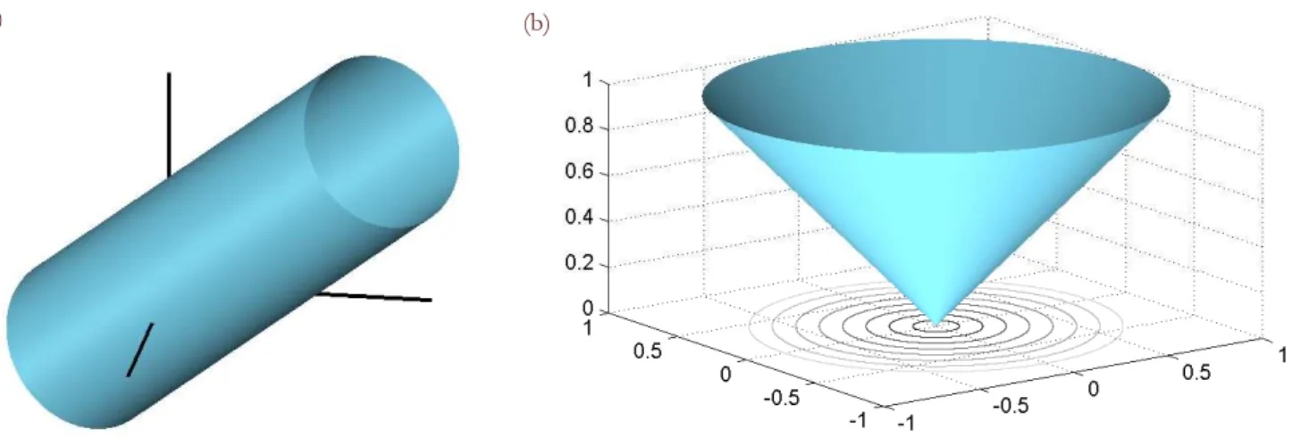
Figure 5: Von Mises yield function. (a) Yield surface; (b) Dissipation function graph.

Figure 6: Von Mises–Tresca (m20) yield function. (a) Yield surface; (b) Deviatoric section of the yield surface; (c) Dissipation

function graph; (d) Unitary level set of the dissipation function.

Fig. 5 shows the corresponding yield surface and dissipation function graph. It is worth noting that the dissipation function results convex, non-negative, zero only at the origin and positively homogeneous of degree one. The latter feature is clear from its cone-like graph.

Von Mises–Tresca yield function

The von Mises–Tresca yield function corresponds to the choice (see [17] and references therein):

(a) (b)

(a) _(b)

(17)

127

 

 1 2



₂ ₂ ₂



1 2

ˆ 1 2 3

2

2 3 3

m m

m

m _d m m

g  d d



  

σ (B2)

where

 

ˆ



ˆ



2



ˆ





ˆ





ˆ



 

ˆ

1 cos cos 2 3 , cos 2 3 cos 2 3 , 3 cos 2 3 cos

d  _σ  _σ  d  _σ   _σ  d  _σ   _σ (B3)