Spatial Structure of Above-Ground Biomass
Limits Accuracy of Carbon Mapping in
Rainforest but Large Scale Forest Inventories
Can Help to Overcome
Stéphane Guitet1,2,5
*, Bruno Hérault3, Quentin Molto4, Olivier Brunaux1, Pierre Couteron5
1Office National des Forêts (ONF), R&D department, Cayenne, French Guiana,2Institut National de la Recherche Agronomique (INRA), UMR Amap, Montpellier, France,3Centre de coopération Internationale de la Recherche Agronomique pour le Développement (CIRAD), UMR EcoFoG, Kourou, French Guiana,
4CIRAD, UR BSEF, Montpellier, France,5Institut de Recherche pour le Développement (IRD), UMR Amap, Montpellier, France
Abstract
Precise mapping of above-ground biomass (AGB) is a major challenge for the success of REDD+ processes in tropical rainforest. The usual mapping methods are based on two hypotheses: a large and long-ranged spatial autocorrelation and a strong environment influ-ence at the regional scale. However, there are no studies of the spatial structure of AGB at the landscapes scale to support these assumptions. We studied spatial variation in AGB at various scales using two large forest inventories conducted in French Guiana. The dataset comprised 2507 plots (0.4 to 0.5 ha) of undisturbed rainforest distributed over the whole region. After checking the uncertainties of estimates obtained from these data, we used half of the dataset to develop explicit predictive models including spatial and environmental effects and tested the accuracy of the resulting maps according to their resolution using the rest of the data. Forest inventories provided accurate AGB estimates at the plot scale, for a mean of 325 Mg.ha-1. They revealed high local variability combined with a weak autocorre-lation up to distances of no more than10 km. Environmental variables accounted for a minor part of spatial variation. Accuracy of the best model including spatial effects was 90 Mg.ha-1 at plot scale but coarse graining up to 2-km resolution allowed mapping AGB with accuracy lower than 50 Mg.ha-1. Whatever the resolution, no agreement was found with available pan-tropical reference maps at all resolutions. We concluded that the combined weak auto-correlation and weak environmental effect limit AGB maps accuracy in rainforest, and that a trade-off has to be found between spatial resolution and effective accuracy until adequate
“wall-to-wall”remote sensing signals provide reliable AGB predictions. Waiting for this, using large forest inventories with low sampling rate (<0.5%) may be an efficient way to increase the global coverage of AGB maps with acceptable accuracy at kilometric resolution.
OPEN ACCESS
Citation:Guitet S, Hérault B, Molto Q, Brunaux O, Couteron P (2015) Spatial Structure of Above-Ground Biomass Limits Accuracy of Carbon Mapping in Rainforest but Large Scale Forest Inventories Can Help to Overcome. PLoS ONE 10(9): e0138456. doi:10.1371/journal.pone.0138456
Editor:Krishna Prasad Vadrevu, University of Maryland at College Park, UNITED STATES
Received:February 27, 2015
Accepted:August 31, 2015
Published:September 24, 2015
Copyright:© 2015 Guitet et al. This is an open access article distributed under the terms of the Creative Commons Attribution License, which permits unrestricted use, distribution, and reproduction in any medium, provided the original author and source are credited.
Data Availability Statement:All relevant data is
available from Dryad: doi:10.5061/dryad.38578under
data files: Forest Inventories used for AGB estimates in French Guiana.
Introduction
Estimating carbon flux due to afforestation, deforestation, and forest degradation requires quantifying above-ground biomass (AGB), especially over extensive areas of old-growth tropi-cal forests which have high but varied carbon stocks and are threatened by a rapidly changing
land-use dynamics in many countries [1]. Precise mapping of AGB in tropical rainforest is a
thus major challenge for the success of REDD+ processes [2]. The objectives set by
interna-tional organizations are very ambitious but they are faced the inability of many tropical
coun-tries to produce accurate maps of AGB [3]. In fact, in most countries where land-use changes
and forestry are major contributors to greenhouse emissions, biomass pools are poorly
reported (i.e. use thetier 1default value proposed by IPCC—Intergovernmental Panel on
Climate Change), whereas precise estimates based on specific spatial data are required (i.e.
IPCC tier 2 and tier 3 methods [2]).
Many mapping methods based on forest inventories and/or remote-sensing products
have been developed in recent decades [4]. The main techniques, whose applications are not
mutually exclusive and are sometimes combined, are based on: (i) spatial interpolation between
forest plots, generally by inverse-distance weighting [5–7]; (ii) deterministic models using
strat-ification (vegetation maps) or previously mapped predictive ecological variables which are
assumed to influence forest structure and composition [8]; (iii) remote-sensing approaches,
which make it possible to define more homogeneous forest types and/or more efficiently
describe the spatial variation of ecological variables [9,10]. These methods imply heavy
hypoth-eses in terms of biomass distribution, which need to be corroborateda posteriori. Spatial
inter-polation implies that biomass has a strong spatial structure (i.e. is strongly auto-correlated), and deterministic modelling implies that biomass is influenced to varying degrees by the envi-ronment. Remote-sensing approaches often rely on a different base, and aim at more or less direct measurement. The most recent methodological improvements involve remote-sensing data at very high spatial resolution (VHRS), especially LiDAR, which are able to provide direct descriptors of forest structure including tree height, crown size, and tree density, i.e. the main
parameters needed to predict biomass [11,12]. Stand level models analogous to forestry
allome-tries are then calibrated to directly convert the physical signals into biomass or carbon
esti-mates [13,14]. However, the coverage of these VHRS images is usually limited by small swaths
and their high cost per hectare covered. Consequently, they are frequently combined with medium to coarse resolution data which make it possible to upscale local estimates (based on
field data, VHR remote sensing or both) over broader areas [15,16] through the same apriori
hypotheses (i.e. autocorrelation and dependence on the environment). Several products have already been developed at continental scales using these latter methods. They have been
described as a robust basis for national carbon inventories or regional REDD+ projects [15,16].
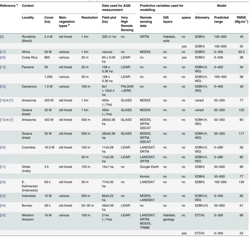
In spite of this progress, the reliability of most of these mapping products has been shown to be questionable. The precision reported for recent maps varied dramatically between 25 and
65 tC.ha-1(i.e. 50 to 130 Mg.ha-1for AGB) depending on the resolution of the output map, the
extent of the area, and the type of vegetation cover (seeTable 1), but comparisons with
inde-pendent validation data often revealed larger bias than the originally reported accuracy [7].
Several problems that limit the reliability of the maps have already been identified: (i)
satura-tion phenomena with certain RS captors at more than 150 t. ha-1[17] (ii) spatial mismatches
between field data (located with GPS) and geo-referenced RS images [18]; (iii) problem of
representativeness of the calibration data due to small plots, usually<0.25 ha [19,20]; (iv) «
dilution bias » when up-scaling from plot areas to VHRS image footprints, due to local
heterogeneity and rugged relief [21]; (v) huge uncertainties at the landscape scale linked to
poor interpolation of scarce field data [22]. Most of these pitfalls and biases are linked to the
structural fundings, Région Guyane). BH benefited from an‘Investissement d’Avenir’grant managed by the Agence Nationale de la recherche (CEBA, ref ANR-10-LABX-0025). The funders had no role in study design, data collection and analysis, decision to publish, or preparation of the manuscript.
Table 1. Overview of recent articles focused on“mapping biomass in tropical forest”.
Referencea Context Data used for AGB
measurement
Predictive variables used for modelling Model Locality Cover (ha) Main vegetation typesb
Resolution Field plot (ha) Very High Remote Sensing Remote sensing data GIS layers
space Allometry Predicted range
RMSE (Mg.ha-1)
[8] Rondônia
(Brazil)
2.4 M old forest 1 km 330 x1 ha no SRTM Habitats,
soils
no f(DBH) 100–600 49
yes f(DBH) 100–600 35
[27] Africa 20 M various 1 km various no MODIS no no f(DBH) 0–350 50.5
[28] Costa Rica 800 various 30 m 83 x 0.09
ha
LiDAR no no yes f(DBH) 0–500 38
[12] Panama 50 old forest 30 m 128 x
0.36 ha
LiDAR no no no f(DBH,H,
WD)
0–400 34
1,256 various 30 m 128 x
0.36 ha
LiDAR no no no f(DBH,H,
WD)
100–400 38
[29] Cameroon 1.5 M various 100 m 8x1
+ 10x0.4 ha
PALSAR +JERS
no no no f(DBH,H,
WD)
0–400 49
[16] in [7] Amazonia 423 M old forest 1 km 493x (1ha)
GLASS MODIS no no varied 50–350 77
Guiana shield
32 M old forest 1 km 493x
(1ha)
GLASS MODIS no no varied 50–350 123
[15] in [7] Amazonia 423 M old forest 500 m 283x0.36 ha
GLASS MODIS,
SRTM, QSCAT
no no f(DBH,H,
WD)
50–350 83
Guiana shield
32 M old forest 500 m 283x0.36
ha
GLASS MODIS,
SRTM, QSCAT
no no f(DBH,H,
WD)
50–350 117
[30] Colombia 16.5 M old forest 100 m 11x0.28
ha
LiDAR LANDSAT,
SRTM
no no f(DBH,H,
WD)
0–280 56
30 m 11x0.28
ha
LiDAR LANDSAT,
SRTM
no no f(DBH,H,
WD)
0–280 82
[31] Ghats
(India)
3 k old forest 125 m 15x1 ha no Google Earth no no f(DBH) 50–650 80
Ikonos no no f(DBH) 50–650 77
[32] E.
Kalimantan (Indonesia)
83 k old forest 30 m 77x0.05
ha
no LANDSAT no no f(DBH) 100–600 130
[33] Indonesia 10 M various 200 m 85x0.25
ha
no MODIS,
LANDSAT
no no f(DBH,H,
WD)
0–450 85
[34] Borneo 28 k old forest 20–30 m 48x0.09
ha
LiDAR no no no f(DBH,H) 50–600 61
[35] Western
Amazon
16 M various 100 m 214x
(1ha)
LiDAR LANDSAT, SRTM, MODIS, TRMM Habitats, geology
no f(TCH) 0–300 66
yes f(TCH) 0–300 53
aonly articles which provided precise information simultaneously on root mean square error (RMSE), resolution, and extent are included. b
“various vegetation types”means the study included explicit samples in savannahs, young plantations or opened/highly degraded forest in addition to forests;“old forest”means the studies focused mainly on old-growth forest (and did not include samples of other vegetation types for calibration and validation).
cDBH for diameter at breast height, H for Height, WD for Wood density or Wood Speci
fic Gravity, TCH for“top-of-canopy height”
autocorrelation hypothesis and to the lack of representativeness of field data, which are gener-ally undersized, mismatched, and above all too scarce and scattered, given the high variability
of forest structure at both local and landscape scales [22]. The spatial structure of biomass at
varying nested scales is key information when designing efficient sampling to ensure the
robustness of calibration. This issue has been widely studied locally [21,23], but studies at the
landscapes scale are lacking [22] because they require the collection of numerous data, which is
costly.
Following the development of forestry in tropical countries, more and more forest manage-ment inventories are being produced by public and private operators and cover large areas,
especially when results from concession-scale operations are lumped together (e.g. [24–26]).
However, the measurements are often not sufficiently precise (local vernacular names are used instead of botanical names, diameter at breast height is recorded by class, and there is no mea-surement of total height). Consequently the uncertainty due to inaccuracy needs to be more precisely assessed but the high repetition rate of the data could compensate for the lack of pre-cision and provide information on the spatial structure of the biomass at landscape scale, as well as solve the problem of representativeness.
For the present study, we used two large forest inventories conducted in French Guiana
dur-ing the periods 1974–1976 and 2006–2012 in 2,507 plots that sampled 1,120 ha over the 8 M
ha undisturbed rainforest. Our aims were to (i) assess the precision of biomass estimates obtained from this kind of forest inventory data; (ii) test the spatial structure of biomass (i.e. auto-correlation in biomass distribution) at various scales in order to assess accuracy as a func-tion of resolufunc-tion; (iii) produce maps at different resolufunc-tions using different predictive models and compare their accuracy with other products, for practical use in REDD+ programmes.
Materials and Methods
Field measurements
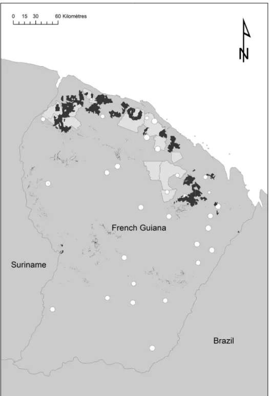
We used two different forest inventories produced by French public organizations(Fig 1). The
first inventory was done by CTFT (Centre Technique Forestier Tropical) between 1974 and
1976 in the northern part of the French Guiana [36]. CTFT data were scanned between 2006
and 2010 and positioned on GIS using original maps. This dataset corresponded to 126,880
trees (DBH20cm) in 1,172 plots 0.5 ha in size.
The second inventory was done between 2006 and 2013 on behalf of ONF (“Office National
des Forêts”: the French national forest agency) to complete regional coverage and better sample
environmental variability [37]. Thirty three sites were selected mostly in the south and east of
French Guiana to cover the geological and climatic conditions poorly sampled by the former CTFT inventories. ONF data represented a total of 1,335 0.4-ha plots where 83,075 trees
(DBH20cm) were measured. All the plots were geo-referenced using a GPS receiver.
These inventories did not include palms and small trees (DBH<20cm). However, they
pre-viously proved to represent minor and reasonably stable proportions of total AGB from 10 to
14% (e.g. [38,39]). Details about these two inventories and the pre-treatments used to control
their quality and homogenise the two datasets are given inS1 Text.
Environmental data
For all plots, we extracted from GIS all environmental variables assumed to influence forest
growth that were freely accessible on available maps (Table 2). For continuous variables, we
computed the mean values over the plot area, while for categorical variables we selected the
majority class. We used a simplified geological map [40] for the substrate; SRTM from NASA
hydraulic basin in log-scale (LOG) and height above the nearest drainage (i.e. HAND [42]);
recent geomorphological maps generated from SRTM [43] to describe landforms and
land-scapes; a broad-scale vegetation map based on SPOT-VEGETATION remote sensing images
Fig 1. Spatial distribution of inventory blocks from CTFT (1974–1976) and ONF (2006–2013).Inventory blocks from CTFT (1974–1976) in pale grey polygons. Complementary inventory campaigns from ONF (2006–2013) in white circles (size represent the effective area covered by transects). Areas disturbed by harvesting or mining between 1974 and 2007 (in black) were removed from the dataset.
[44]; dry season length (DRY) and annual rainfall (RAIN) from TRMM data resampled at
90 m with a bi-cubic method for climatic descriptors [45].
Biomass estimates and uncertainties
We computed above-ground tree biomass (AGBtree) using the generic pan-tropical allometry
(Eq 1) from Chave et al. [47]. As the forest inventories provided approximate data (i.e. class of
DBH instead of precise DBH, no measure for individual height, and vernacular names instead of precise botanical determination to predict wood density), we estimated the uncertainties due to measurement errors. For each tree in a given DBH class, we simulated precise DBH values (DDBHclass) using exponential distribution. Next we sampled height value (HDBHclass/plot) using
a local allometry based on an asymptotic model [48] and calibrated with the plot’s stand
struc-ture [48] (seeS2 Text). We also allocate trees to precise botanical species using a Monte-Carlo
process based on empirical relationships between vernacular names and botanical species,
which also accounts for the expected precision of each vernacular name [49]. We then used the
Global wood density database [50] to compute simulations of mean wood gravity at the plot
scale (WSGplot). Next, for each plot area of Splotha, we computed the above-ground biomass
per hectare (AGBplot) using the determinist model fromEq 2.
AGBtree¼0:0673 ðWSGDBH
2
HÞ0:973 ð1Þ
AGBplot¼
P
DBHclass
P
trees0:0673 ðWSGplotD
2
DBHclassHDBHclass=plotÞ
0:973
Splot
ð2Þ
AGB estimations were repeated 1,000 times for each plot in order to evaluate uncertainties
due to measurement errors. We did not take the errors due to allometry (i.e.Eq 1) into account
because the resulting uncertainty (though very high at the individual tree scale [47,51,52]), was
expected to be cancelled out or at least drastically reduced on such large plots (as suggested by
previous studies [47,51,53,54]). We verifieda posteriorithat this hypothesis was correct and
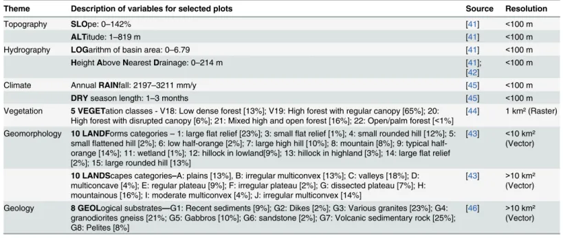
Table 2. Environmental variables tested to predict aboveground biomass.
Theme Description of variables for selected plots Source Resolution
Topography SLOpe: 0–142% [41] <100 m
ALTitude: 1–819 m [41] <100 m
Hydrography LOGarithm of basin area: 0–6.79 [41] <100 m
HeightAboveNearestDrainage: 0–214 m [41];
[42]
<100 m
Climate AnnualRAINfall: 2197–3211 mm/y [45] <100 m
DRYseason length: 1–3 months [45] <100 m
Vegetation 5 VEGETation classes - V18: Low dense forest [13%]; V19: High forest with regular canopy [65%]; 20: High forest with disrupted canopy [6%]; 21: Mixed high and open forest [16%]; 22: Open/palm forest [<1%]
[44] 1 km² (Raster)
Geomorphology 10 LANDForms categories–1: largeflat relief [23%]; 3: smallflat relief [1%]; 4: small rounded hill [12%]; 5: smallflattened hill [2%]; 6: low orange [2%]; 7: large high hill [10%]; 8: mountain [8%]; 9: typical half-orange [14%]; 11: wetland [1%]; 12: hillock in lowland[9%]; 13: hillock in highland [3%]; 14: largeflat relief [2%]; 15: large rounded hill [13%]
[43] <10 km² (Vector)
10 LANDScapes categories–A: plains [13%], B: irregular multiconvex [13%]; C: valleys [18%]; D: multiconcave [4%]; E: regular plateau [9%]; F: irregular plateau [2%]; G: dissected plateau [7%]; H: mountainous [16%]; I: moderate multiconvex [4%]; J: irregular multiconvex [14%]
[43] >10 km²
(Vector)
Geology 8 GEOLogical substrates—G1: Recent sediments [9%]; G2: Dikes [2%]; G3: Various granites [23%]; G4: granodiorites gneiss [21%; G5: Gabbros [10%]; G6: sandstone [2%]; G7: Volcanic sedimentary rock [25%]; G8: Pelites [8%]
[46] >10 km² (Vector)
that propagating all uncertainties in our tests didn’t change our results (seeS3 Text). Despite
the approximate measurements of forest inventories, coefficient of variation (CV) of AGB
esti-mates at the plot scale rarely exceeded 17% for CTFT data and 10% for ONF data. So in the
worst case, the confidence interval of mean AGB estimates at 95% for plots did not exceed 6
Mg.ha-1. Finally, in order to compare our results with previous similar studies (seeTable 1), we
simply used mean AGB estimates for plots and didn’t propagate uncertainty in the following
tests (seeS1 Dataset).
Statistical analyses
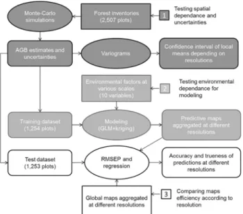
Statistical analyses followed three steps that are summarized inFig 2. In the first step we used
all our data to produce variograms in order to examine the spatial structure of biomass and its
consequences in terms of accuracy for interpolating from field data (dark grey onFig 2). In a
second step we used half of our data (training dataset) to calibrate prediction models in order to produce AGB maps at different resolutions and to evaluate the influence of environment
fac-tors on AGB variation (medium grey onFig 2). In the last step we used the second half of our
data (test dataset) to compute Residual Mean Square Error of Prediction (RMSEP) and regres-sions in order to test the accuracy of our maps at different resolution and to compare it with
the accuracy of extant global maps (from Baccini [15] and Saatchi [16]).
Testing spatial dependences and uncertainties due to local variability. To detect spatial dependences in biomass distribution, we performed a variogram (semi-variance) analysis
(package geoR–[55]) using all our data. Mean semi-variance was computed for 10 distance
classes (i.e. limits at 500 m, 1 km, 2, 4, 8, 16, 32, 64, 120, and 240 km) and compared with the null hypothesis of an absence of spatial structure simulated by 1,000 randomizations of AGB
values between plots. At any distance class L (between L1km and L2km), having the observed
semi-variance under the random confidence interval indicated significant auto-correlation, whereas semi-variance above this confidence interval indicated significant over-dispersion.
We then assessed the implication of the spatial structure for the computation of the theoret-ical confidence interval of the local AGB mean. We first generated systematic grids with
Fig 2. Flowchart followed for statistical analyses.The grey colours indicate the different steps of analysis. Input data are represented in rectangles, analysis in ellipse and outputs in rounded boxes.
different cell-sizes (resolution R = 0.5 km–1 km–2 km–4 km–8 km) and selected all cells including at least three plots. This yielded 142 to 316 cell values per grid. We then computed
the coefficient of variation (CV) and the 95% confidence interval of the local estimates (IC95%)
usingEq 3, and we modelled the relationship between IC95%, N and R using log-log
regres-sions.
IC95%¼tN;95 CV
p
N ð3Þ
Modeling biomass with GLM and ordinary kriging. We tested general linear models (GLM) of every possible first-order combination of environmental variables (package R stats
and glmulti—[56]) in order to (i) test to what extent environmental effects can explain biomass
spatial variation; (ii) interpret the main significant effects; (iii) produce the most efficient pre-dictive map. We used the Akaike Information Criterion (AIC) to select the best and most
parsi-monious model and verifieda priorihypotheses: normality of the residues
(Kolmogorov-Smirnov test), heteroscedasticity (Breusch-Pagan test) and independence of the residues (var-iogram). We tested the different terms of the model using ANOVA.
In a first step we included the type of inventory (i.e. CTFT versus ONF) in the GLM in addi-tion to environmental factors in order to test the bias that could be introduced by joining old and new field data. The variable was selected in the best model but its effect proved to be very limited and non-significant regarding ANOVA-test (coefficient -12.7, ddl = 1, F value = 2.32, p = 0.127). We then renewed the test without this factor. The new model led to the selection of the same environmental factors than in the first test with a slight increase in AIC (11541 versus
11540) and similar predictions (no bias—R² = 0.985). As a consequence, we neglected
inven-tory effect thereafter.
As spatial correlation was detected in the residues of GLM, we added a spatial component k
(s) to the deterministic terms of the model (i.e.Eq 4with estimated meanμand environmental
effectsγefor each of the variables xe). We modelled k(s) by ordinary kriging as proposed by [8].
We postulated an exponential function for the covariance model (i.e.Eq 5withτ= nugget,σ² =
sill,φ= range) and fitted the terms of the model to the observed variogram of residues using
ordinary weighted least squares (package R geoR–[55]).
As a result, our final model to predict AGB at the location s, noted y(s), is a kriging-regres-sion model (KR) which took the following form:
yðsÞ¼mþ XE
e¼1gexeðsÞ þkðsÞ ð4Þ
With the covariance model of k following the exponential form:
gð Þ ¼d tþðs2 tÞ 1 exp d
φ
ð5Þ
We used half of our dataset to calibrate this model, systematically selecting one plot out of two (training set) and reserved the rest (test dataset) to compute the root mean square error of prediction (RMSEP) of our model in the validation step. We preferred this conservative method to more sophisticated cross-validation ones (e.g. one-out-of bag) in order to limit the
risk of over fitting (e.g. [35]).
Mapping and comparing our model with other models at different scales. We first applied our GLM and KR models to produce maps at the finest possible resolution (30 m) on GIS. We then produced coarse-grained maps by local averaging at different resolutions (1 km,
process on pan-tropical maps produced by Baccini [15] and Saatchi [16] and aligned the four maps, in order to compare their accuracy with ours at the different resolution For each resolu-tion, we then selected cells featuring more than three validation plots from the test dataset and we computed RMSEP using the local means. We also examined the precision and trueness of the maps using respectively the correlation coefficient (R²) and slope of linear regression between the predictions and the test dataset.
Finally, to evaluate the practical relevance of the different maps at operational scales (i.e. at the scale of a forest concession, between 10,000 and 100,000 ha, or at the scale of a local forest management project, between 1,000 and 5,000 ha), we computed the same indicators (RMSEP, r², slope of regression) for the range of areas displayed by the CTFT inventory blocks (166 to 800 km²) and for the ONF inventory sites (10 to 47 km²). We supposed these areas to be within
the range leading from forest concession to large REDD project areas (>100 km²) or local
REDD project areas (10–50 km²). We also compared the biomass estimates obtained with our
training set and those obtained with our test set for these areas to see the absolute accuracy we could expect from forest inventories at these scales.
Results
A high local variability and a weak spatial structure led to large
uncertainties in local biomass estimates
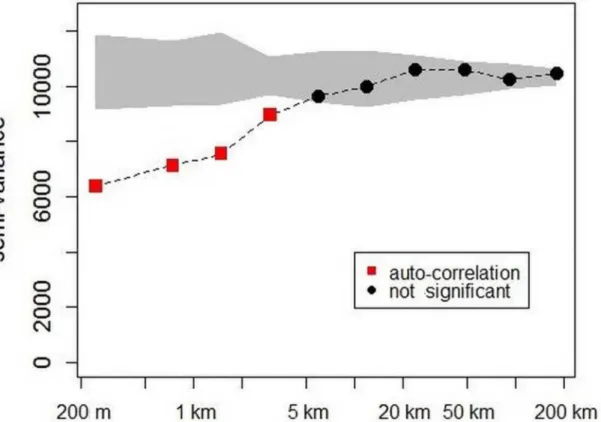
Variograms applied on the mixed datasets(Fig 3)showed high and significant semi-variance
at the beginning of the curve (i.e. nugget of about 6,000 equivalent to a difference of about
110 Mg.ha-1between neighbouring plots, located less than 500 m apart). Semi-variance
increased rapidly up to 20 km and remained a fairly stable from 20 km to 200 km (i.e. sill of
about 10,000 equivalent to a difference of about 140 Mg.ha-1) approximating the overall
vari-ance. Comparison with 1,000 randomizations indicated a significant autocorrelation for dis-tances of less than 5 km and no other significant effect for larger disdis-tances. This shape of variogram with high nugget effect (local variability) and short range of auto-correlation corre-sponded to a weak spatial structure (i.e. very limited spatial dependence in biomass variation).
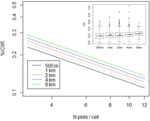
In accordance with the previous variogram, CV of local AGB estimates had a quite high mean value (about 21%) when computed on the 0.5 km resolution grid. It increased very
slowly, up to 27%, when we increased the size of the grid cells from 1 km to 8 km(Fig 4).
Modelling IC95%(relative confidence interval of local AGB estimates) from the number of field
plots (N) and grid resolution (R), led to the log-log model (r² = 0.82, F = 232, DF = 99,
p<0.001, AIC = -24):
logðIC95%Þ ¼ 0:59277 0:59128logðNÞ þ0:04988logðRÞ ð6Þ
We observed that %IC95decreased mainly with an increase in the number of calibration
points and increased slowly with resolution(Fig 4). As a result, for the same sampling density,
the uncertainty of local biomass estimates was halved when the cell size was doubled (e.g.
IC95%= 24% for three plots on average in 1 km-cells and IC95%= 13% for 12 plots in 2
km-cells).
The environment accounts for a significant but minor part of spatial
variation in biomass
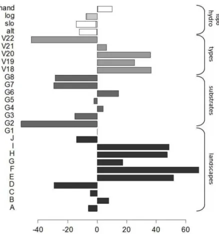
The best GLM selected to predict biomass variation with environmental variables explained a small but significant proportion of variance when fitted on the training set (R² = 0.09,
season index and annual rainfall were excluded from the model(Fig 5). Geomorphological
landscapes had the strongest effect on biomass (F = 6.0664, DF = 10, p<0.001) and displayed
marked contrasts at large scales between (i) on the one hand, regions dominated by mountains (H), plateaus (E,F,G), or smoothed multi-convex landscapes (I) with high biomass; and (ii) on the other hand, plains (A), valleys (C), multi-concave (D) and marked multi-convex landscapes (B,J) with low biomass. Low HAND (height above the nearest drainage) and high LOG (loga-rithm of basin area), which mainly point to seasonally flooded forests, were also highly
influen-tial at the local scale with a significant negative effect (respectively F = 11.3495, p<0.001 and
F = 9.9309, p<0.01). GEOL (Geology) had a significant but limited effect driven by the“dykes”
category (G2), which corresponded to an extremely hard localized substrate with significantly
lower biomass (F = 2.5477, DF = 7, p<0.05). Similarly, VEGET (vegetation type) had only a
slight effect mainly driven by type 22 which exhibited very low biomass (F = 2.8287, DF = 5,
p<0.05) and corresponded to“open forests mixed with palm forests”, mainly located in the
southern part of French Guiana. Altitude and slope had the weakest effects (respectively
F = 3.5036, p<0.1 and F = 2.5405, p = 0.111).
The variogram computed on the residuals of the model still showed significant spatial
dependence for distances of less than 2 km(Fig 6). We modelled this residual structure by
kri-ging-regression (KR) using an exponential covariance function (τ= 6500,σ= 3205,φ= 1991–
fixed kappa = 0.5).
As a result, when we applied the GLM (deterministic part of the calibrated model) to the test set, we obtained a quite large RMSEP of 99t MS/ha and a poor adjustment (r² = 0.04,
DF = 1251, p<0.001, slope = 0.063). When we used the complete model KR, we increased the
Fig 3. Variogram of biomass estimates from 500 m to 200 km according to distance classes.The grey shape shows the confidence interval expected for each distance class under the null hypothesis (1,000 randomizations). The red squares indicate significant auto-correlation and the black circles imply no significant correlation.
accuracy of the model (RMSEP = 90t MS/ha) with a better adjustment (r² = 0.20, DF = 1251,
p<0.001, slope = 0.208). However, as the practical range of auto-correlation used in kriging is
short, it did not enable residual error to be predicted beyond a distance of 7 km around the sampling locations. Consequently, model accuracy was only actually improved by the spatial component in a small part of the territory located near the sampling areas used for calibration
(Fig 7).
Coarse-graining improved the accuracy of maps
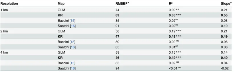
The pan-tropical maps at their original resolution (i.e. 1km) were poorly correlated with the
test dataset (RMSEP>80, R² = 0.02 and slope0.1) whereas the accuracy of our complete
model (i.e. KR) was largely improved at this resolution (RMSEP = 63, R² = 0.35 and slope = 0.55).
The same results were obtained with 2-km resolution cells(Table 3andFig 8). Thanks to
coarse-graining, our models were more accurate than at the finest resolution (RMSEP was reduced by 25% for GLM and 30% for KR compared with 1-km resolution), with better
preci-sion (r² = 0.19 and 0.48 for GLM and KR respectively with p<0.001 in both cases). However
the regression slopes kept the same value as at 1-km resolution (i.e. about 0.2 for GLM and about 0.5 for KR), indicating a dilution bias effect that could not be reduced. As a result, bias was zero for mean values but systematically negative for the highest values and positive for the
lowest values (Fig 8). At and above 4-km resolution, all statistics of adjustment were degraded
or saturated on all maps (RMSEP, R² and the same or worse slope than previously).
Fig 4. Estimation of coefficient of variation and confidence interval of local mean according to grid resolution.Inset boxplot shows CV of local biomass estimates according to grid resolution. Main part shows the fitted values confidence interval of the local mean according to the model log (IC95%) = -0.59277–0.59128
*log (N) + 0.04988*log (R) from N = 3 to 20 and R = 0.5 km to 8 km.
Satisfactory accuracy can be achieve for REDD+ operational scales
The comparison of our test dataset and training dataset showed that forest inventories with asampling rate of between 0.1 and 0.5% estimated biomass with an accuracy<10% for large
blocks (>100 km²) and for a large majority of 10 to 50-km² sites (respectively RMSE = 10 and
26 Mg.ha-1–Table 4). At these operational scales, our complete KR model estimated total
bio-mass with good accuracy (RMSE = 31 Mg.ha-1for ONF sites and 18 Mg.ha-1for CTFT blocks),
whereas simple GLM led to larger errors (Table 4). AGB estimates obtained with pan-tropical
maps were absolutely not correlated with our test dataset, with the exception of Baccini’s map
for areas between 10–50 km² (r² = 0.15–p<0.05).
Discussion
High local variability limits the accuracy of biomass maps
The spatial structure of aboveground biomass (AGB) has already been shown to be highly vari-able at spatial resolutions less than 250 m when measured in forest plots ranging from 6 to 50
ha in size [19,21]. The high local variability can be explained by gap-phase dynamics which
cre-ate a mosaic of eco-units [19,58]. This local variability implies that significant“dilution bias”
will occur when small plots (i.e. substantially less than 0.5 ha) are used to calibrate models to be applied over larger areas. Upscaling leads to underestimation of the spatial variance of AGB
Fig 5. Coefficients of the selected GLM that predict biomass from environmental variables.Grey bars and brackets indicate groups of modalities related to the different categorical variables. For continuous topographical and hydrographical variables (HAND, LOG, SLOpe and ALTitude) the coefficient value is multiplied by the mean of the variable.
in the models [21]. Our study proves that AGB variability is already very high at spatial
resolu-tions of between 200 and 500 m and increases even more at more than 5 km (Fig 3) whereas
one might expect that this effect, which is linked to forest dynamics, would be mitigated over
large areas (i.e.>1 km²). As a result,“dilution bias”is likely to occur even when large forest
plots i.e. ca. 1 ha, are used to calibrate models with standard satellite remote-sensing data, as it
is widely recommended [21]. Dilution bias is also to be expected when a few small footprints
covering areas of the same order of magnitude as field plots are used as sampling units to cali-brate larger footprints (e.g. airborne LiDAR transects or GLASS footprints used to calicali-brate MODIS or LANDSAT pixels). This helps explain why pan-tropical maps, which are based on double upscaling (from field to high resolution RS and then to medium resolution RS) fail to
capture the forest spatial variability of AGB with acceptable accuracy [7].
The high local variability measured in our forest inventory plots (average standard deviation
above 100 Mg.ha-1), cannot be the result of unexpected noise in the inventory data, because (i)
the sizes of our plots, between 0.4 and 0.5 ha, are sufficient to limit in-and-out effects for large
trees [20]; (ii) uncertainties and local variability computed at the plot scale are consistent with
previous studies [59]; (iii) the local CV measured within 500 m-resolution cells was of the same
order of magnitude as reported for 200 m in other studies based on permanent plots in a
tropi-cal forest [21]. Obviously, the heterogeneity between the different sources of data has been
cor-rectly controlled since no important bias due to inventory was detected in the analysis. This is in accordance with previous study which detected only a slight increase in AGB during the past
decade in our region (<0.9 Mg.ha-1.y-1) with no statistical significance [39]. Moreover, we
Fig 6. Variogram of GLM residuals from 500 m to 200 km according to distance classes.The grey shape indicates values expected under the null hypothesis of absence of spatial structure (1,000 randomizations). The red squares indicate significant auto-correlation and the black circles no significant structure. The dashed line represents the fitted exponential model used to predict the spatial error term.
verified that errors due to allometry and measurements led to very limited uncertainties (i.e.
<15%).
We therefore conclude that this high local variance is not an artefact, but is likely due to the
heterogeneous forest structure [22], which in turn, could be explained by (i) local topographic
and hydrologic effects (included in our GLM with altitude, HAND and basin area); (ii) the dis-tribution of big trees which often exhibit aggregative patterns driven by population dynamics
and species dispersion in the long term [60]; (iii) large-scale natural forest disturbances such as
landslides or blowdown, even if gaps of more than 1 ha have been shown to be quite rare in
northern Amazonia [61].
Environmental factors are partly efficient to capture this structural variability, rather due to stochastic processes. In fact, the deterministic part of our model explained a modest part of the variance. However, our model was able to detect contrasts along the waterlogging gradient on
Fig 7. Map of AGB (Mg.ha-1) in French Guiana based on the complete model (KR).Local darker or paler areas correspond to spatial error terms that can
be modelled only within a short distance of the calibration plots and are null over most of the area.
the topographic sequence [62,63] as well as large scale variations at the landscape scale [64]. Nevertheless, as shown in previous studies, even in the case of strong environmental contrasts monitored at fine scale (e.g. waterlogged vs. never flooded locations or white sand vs. other terra firme forests) pure environmental effects only explain a small fraction of variations in
AGB and interact largely with more important structural effects [65].
The important consequence of major variations in AGB at short distance, as evidenced by
the present study, which corroborates another recent one [22], is that any statistical
interpola-tion between scare field reference points will remain imprecise whatever the accuracy of the field measurements. The only way to enhance precision is to combine geo-statistical interpola-tion (e.g. kriging) with the most relevant spatialized environmental informainterpola-tion, as exemplified in the present study. Reciprocally, incorporating a spatial component in the biomass model is an effective way to mitigate the problem of weakly environmentally structured variation in
AGB and to substantially improve its efficiency [8,35]. However, we showed that this
improve-ment is limited to a short distance around the reference points, because of the short autocorre-lation range (i.e. a few kilometres).
Sampling design and spatial resolution have to be adapted to capture
AGB spatial structure
The most cost-effective way to capture and control the local variability is to adapt the resolu-tion of the output AGB map to average out local variability. In other words, a trade-off needs to be found between spatial resolution and effective accuracy. On the one hand, reducing out-put resolution minimizes local variance, but on the other hand, enlarging resolution helps cali-brate the model with more precision by multiplying the number of field plots per
calibration-cell, which is the most efficient way to reduce the confidence interval of local estimates(Fig 4).
In our case, a 2-km resolution (4 km²) appears to be the optimal trade-off between a minimum
RMSEP and maximum adjustment (r² and slope approaching 1—seeFig 8andTable 2) for
calibration. From a practical point of view, this means that AGB maps should not target a reso-lution (output cell size) of less than few kilometres otherwise there is a risk of very high uncer-tainty at individual cell level that will result in a poor calibration step.
Table 3. Accuracy of the different maps for different cell resolutions.
Resolution Map RMSEPa R² Slopea
1 km GLM 74 0.09** 0.21
KR 63 0.35*** 0.55
Baccini [15] 85 0.02ns 0.08
Saatchi [16] 91 0.02ns 0.10
2 km GLM 58 0.19*** 0.21
KR 47 0.48*** 0.49
Baccini [15] 80 0.02ns 0.06
Saatchi [16] 85 0.01ns 0.06
4 km GLM 59 0.15*** 0.14
KR 46 0.49*** 0.40
Baccini [15] 85 0.02ns 0.04
Saatchi [16] 94 <0.01ns -0.02
aThe root mean square error of prediction (RMSEP) indicates the overall accuracy, the R² indicates the precision, and the slope indicates the trueness of
Moreover, our results suggest that regular systematic sampling is not the best way to cali-brate AGB maps. For instance, to accurately calicali-brate a model with less than an average of 5% error at a 2-km resolution, more than 75 plots are necessary per calibration cell, 20 plots for 10% and 5 plots for 20%, which corresponds to a sampling rate of 8%, 2% and 0.5% respec-tively. Such very high sampling rates required to obtain accurate local means for calibration,
are not economically sustainable for very large areas [22]. A multi-scale stratified sampling
Fig 8. Comparison of AGB values predicted by the different maps at 2-km resolution with test dataset.Aboveground biomass (AGB) means at cell level for the test set are compared to the values predicted by the different maps at 2-km resolution: from the top left to the bottom right—KR, GLM, Baccini [15] and Saatchi [16]. The red line indicates the 1:1 relationship (expected slope). The size of the circles indicates the number of plots for each cell in the test set (from 3 for the smallest to 12 for the biggest).
design appears to be a better way of ensuring both a sufficient sampling rate for local calibra-tion and sufficient general coverage to account for the broad-scale patterns of variacalibra-tion in AGB.
Achieving“wall-to-wall”LiDAR over large areas is a reliable alternative way to address
these methodological limits in the medium term [66]. However, a significant gap still exists
between the complexity and cost of this method on the one hand, and the actual capacity of
developing countries to implement it on large areas on the other hand [3]. Here, using large
forest inventories even with a quite low sampling rate (i.e. about 0.01% for the whole territory and from 0.1 to 0.4% locally) we succeeded in producing AGB maps with acceptable RMSEP
ranging from 47 to 58 Mg.ha-1(i.e. 22 to 28 MgC.ha-1that to say, a relative error of 15% to
20%) at a 2-km resolution depending on the distance from the nearest sampled area. As a matter of fact, for operational management of forest resources at local to national scales (e.g. evaluation of biomass for a REDD+ project or LULUCF national monitoring) rapid forest inventories with suitable design may suffice to produce accurate estimates at the appropriate resolution for an output map.
Combining remote-sensing and large scale forest inventories can
improve the accuracy of biomass maps
Our review of literature focusing on“biomass mapping in tropical forest”, shows that RMSE
hardly reach 75Mg.ha-1in old-growth forests (i.e. a relative error of about 20%), for a 1-km
res-olution or less(Table 1). The performance obtained with our forest inventories, even at 1-km
resolution, is better than the majority of biomass maps in the literature [7,15,16,31–33]. Most
studies which report RMSE lower than 75Mg.ha-1, include different vegetation types such as
savannahs, opened forest or young plantation, thus mechanically reducing absolute RMSE (e.g. [28,29] inTable 1), or having to deduce AGB from rough DBH-based allometries that do not account for variations in wood density and height within the forest and hence artificially reduce
actual variance (e.g. [8,27,28] inTable 1). The most efficient AGB maps are based on the“
wall-to-wall”LiDAR method, but remain very limited in extent, i.e. to only a few km² [28,34].
How-ever, a better performance was reported for two maps covering larger areas with RMSE down
to 55 Mg.ha-1(i.e. 27 MgC.ha-1) at 100-m resolution, using LiDAR to calibrate AGB estimates
for forest strata based on LANDSAT and SRTM data [30,35]. These two studies concluded that
the final upscaling step is critical to ensure the efficiency of biomass mapping and to better
Table 4. Evaluation of the accuracy of the different models at operational scales.
Scale Estimates RMSEPa R² Slopea
Small project, production units (10–50 km²) training set 26 0.67*** 0.868
GLM 40 0.32*** 0.339
KR 31 0.64*** 0.551
Baccini [15] 61 0.15* 0.155
Saatchi [16] 70 <0.01ns 0.079
Large project, concessions (>100 km²) training set 10 0.93*** 0.885
GLM 40 0.59** 0.103
KR 18 0.90*** 0.390
Baccini [15] 74 <0.01ns -0.037
Saatchi [16] 56 0.07ns -0.118
aThe root mean square error of prediction (RMSEP) indicates the overall accuracy, the R² indicates the precision, and the slope indicates the trueness of
the models. The significance of the adjusted-R² was tested with a F test (***p<0.001,**p<0.01,*p<0.05, ns = non-significant)
capture spatial autocorrelation to fully transform the potential display by LiDAR altimetry into local AGB predictions at a broad scale.
Our results suggest two ways of improving this upscaling process. First, holistic and multi-scale geomorphological maps can provide an efficient basis for preliminary forest stratification to guide LiDAR acquisition as well as the sampling of field data. This preliminary stratification
step is too often limited toa prioriexpert-based stratification (e.g. altitude threshold,
catch-ment basin delimitation, etc.). A formalized geomorphological analysis based on full-resolution SRTM (as done here) would help define precise and objective relief stratification (e.g. a plateau vs. a multi-convex landscape) while subjectivity can be controlled by using image analysis
tech-niques to characterize and classify landforms (see for instance [43,67,68]). This would also
make it possible to delimit local habitats (i.e. terra firme vs. seasonally flooded forests), thus
reducing within-strata variability [38]. Second, our results demonstrate that field plots in forest
inventories are a reliable source of accurate field measurements of AGB. Such field data can thus be used to locally calibrate and validate LiDAR allometry (leading from canopy altimetry metrics towards AGB) as well as any kind of biophysical information derived from remote-sensing data of sufficient resolution that can contribute to AGB mapping (e.g. canopy texture
as exemplified in [31,69]). Future progress will indeed rely on smart sampling and upscaling
schemes from highly informative (regarding forest structure and biomass mapping) albeit costly data sources such as field inventories and small footprint LiDAR flight lines, to satellite remote sensing information of higher affordability and replicability.
Given such strong local variations in AGB along with short range autocorrelation, the upscaling scheme is indeed critical, and understanding the relationships between variations in above-ground biomass and landscape patterns is a promising way to base the upscaling process on broad scale drivers of AGB variations via variables which can conceptually and statistically be derived from worldwide databases and satellite remote sensing. Combining forest invento-ries along transects with LiDAR flight lines could be an efficient way to improve the global cov-erage of AGB maps of tropical forests while maximizing field datasets and capturing cryptic regional variations (e.g. patterns in wood density, changes in allometry between forest types) that are easily overlooked without an extensive integrated sampling strategy.
Supporting Information
S1 Dataset. Aboveground biomass estimates for the 2507 plots.The file provides 1,000 esti-mates of AGB for the 2507 plots and specifies the geographic coordinates of the centre of the plot (WSG84UTM22N) and the area of the plot (ha).
(XLSX)
S1 Text. Details about field data.
(DOCX)
S2 Text. H:D sub-model used in allometry.
(DOCX)
S3 Text. Propagation of errors due to allometry.
(DOCX)
Acknowledgments
Author Contributions
Conceived and designed the experiments: SG BH. Performed the experiments: SG OB. Ana-lyzed the data: SG QM. Contributed reagents/materials/analysis tools: BH PC. Wrote the paper: SG BH PC QM OB.
References
1. Gibbs HK, Brown S, Niles JO, Foley JA. Monitoring and estimating tropical forest carbon stocks: mak-ing REDD a reality. Environmental Research Letters. 2007; 2(4):045023.
2. Baker DJ, Richards G, Grainger A, Gonzalez P, Brown S, DeFries R, et al. Achieving forest carbon information with higher certainty: A five-part plan. Environmental Science & Policy. 2010; 13(3):249–
60. doi:http://dx.doi.org/10.1016/j.envsci.2010.03.004
3. Romijn E, Herold M, Kooistra L, Murdiyarso D, Verchot L. Assessing capacities of non-Annex I coun-tries for national forest monitoring in the context of REDD+. Environmental Science & Policy. 2012; 19–
20(0):33–48. doi:http://dx.doi.org/10.1016/j.envsci.2012.01.005
4. Qureshi A, Badola R, Hussain SA. A review of protocols used for assessment of carbon stock in for-ested landscapes. Environmental Science & Policy. 2012; 16:81–9.
5. Glenday J. Carbon storage and emissions offset potential in an East African tropical rainforest. For Ecol Manag. 2006; 235(1–3):72–83. PMID:CCC:000242050600007.
6. Malhi Y, Wood D, Baker TR, Wright J, Phillips OL, Cochrane T, et al. The regional variation of above-ground live biomass in old-growth Amazonian forests. Global Change Biology. 2006; 12(7):1107–38.
7. Mitchard ET, Feldpausch TR, Brienen RJ, Lopez‐Gonzalez G, Monteagudo A, Baker TR, et al. Markedly divergent estimates of Amazon forest carbon density from ground plots and satellites. Glob Ecol Biogeogr. 2014.
8. Sales MH, Souza CM Jr, Kyriakidis PC, Roberts DA, Vidal E. Improving spatial distribution estimation of forest biomass with geostatistics: A case study for Rondônia, Brazil. Ecol Model. 2007; 205(1):221–
30.
9. Saatchi S, Houghton R, Dos Santos Alvala R, Soares J, Yu Y. Distribution of aboveground live biomass in the Amazon basin. Global Change Biology. 2007; 13(4):816–37.
10. Saatchi S, Malhi Y, Zutta B, Buermann W, Anderson L, Araujo A, et al. Mapping landscape scale varia-tions of forest structure, biomass, and productivity in Amazonia. Biogeosciences Discussions. 2009; 6 (3):5461.
11. Proisy C, Couteron P, Fromard F. Predicting and mapping mangrove biomass from canopy grain analy-sis using Fourier-based textural ordination of IKONOS images. Remote Sens Environ. 2007; 109 (3):379–92.
12. Mascaro J, Detto M, Asner GP, Muller-Landau HC. Evaluating uncertainty in mapping forest carbon with airborne LiDAR. Remote Sens Environ. 2011; 115(12):3770–4.
13. Asner GP, Mascaro J, Muller-Landau HC, Vieilledent G, Vaudry R, Rasamoelina M, et al. A universal airborne LiDAR approach for tropical forest carbon mapping. Oecologia. 2012; 168(4):1147–60. doi: 10.1007/s00442-011-2165-zPMID:22033763
14. Vincent G, Sabatier D, Rutishauser E. Revisiting a universal airborne light detection and ranging approach for tropical forest carbon mapping: scaling-up from tree to stand to landscape. Oecologia. 2014; 175(2):439–43. doi:10.1007/s00442-014-2913-yPMID:WOS:000336378800001.
15. Baccini A, Goetz S, Walker W, Laporte N, Sun M, Sulla-Menashe D, et al. Estimated carbon dioxide emissions from tropical deforestation improved by carbon-density maps. Nature Climate Change. 2012; 2(3):182–5.
16. Saatchi SS, Harris NL, Brown S, Lefsky M, Mitchard ETA, Salas W, et al. Benchmark map of forest car-bon stocks in tropical regions across three continents. Proceedings of the National Academy of Sci-ences. 2011; 108(24):9899–904. doi:10.1073/pnas.1019576108
17. Kasischke ES, Melack JM, Dobson MC. The use of imaging radars for ecological applications—A review. Remote Sens Environ. 1997; 59(2):141–56. doi:10.1016/s0034-4257(96)00148-4PMID: WOS:A1997WQ31800002.
18. Clark DB, Kellner JR. Tropical forest biomass estimation and the fallacy of misplaced concreteness. J Veg Sci. 2012; 23(6):1191–6. doi:10.1111/j.1654-1103.2012.01471.xPMID:WOS:000310798600019.
20. Baraloto C, Molto Q, Rabaud S, Hérault B, Valencia R, Blanc L, et al. Rapid simultaneous estimation of aboveground biomass and tree diversity across Neotropical forests: a comparison of field inventory methods. Biotropica. 2013; 45(3):288–98.
21. Réjou-Méchain M, Muller-Landau H, Detto M, Thomas S, Le Toan T, Saatchi S, et al. Local spatial structure of forest biomass and its consequences for remote sensing of carbon stocks. Biogeosciences Discussions. 2014; 11(4):5711–42.
22. Marvin DC, Asner GP, Knapp DE, Anderson CB, Martin RE, Sinca F, et al. Amazonian landscapes and the bias in field studies of forest structure and biomass. Proceedings of the National Academy of Sci-ences. 2014; 111(48):E5224–E32. doi:10.1073/pnas.1412999111
23. Chave J, Condit R, Lao S, Caspersen JP, Foster RB, Hubbell SP. Spatial and temporal variation of bio-mass in a tropical forest: results from a large census plot in Panama. Journal of Ecology (Oxford). 2003; 91(2):240–52. PMID:20033060325.
24. Réjou-Méchain M, Pélissier R, Gourlet-Fleury S, Couteron P, Nasi R, Thompson JD. Regional variation in tropical forest tree species composition in the Central African Republic: an assessment based on inventories by forest companies. J Trop Ecol. 2008; 24:663–74. doi:10.1017/s0266467408005506 PMID:WOS:000261254400009.
25. Maniatis D, Malhi Y, Saint André L, Mollicone D, Barbier N, Saatchi S, et al. Evaluating the Potential of Commercial Forest Inventory Data to Report on Forest Carbon Stock and Forest Carbon Stock Changes for REDD+ under the UNFCCC. International Journal of Forestry Research. 2011; 2011:13. doi:10.1155/2011/134526
26. Nogueira EM, Fearnside PM, Nelson BW, Barbosa RI, Keizer EWH. Estimates of forest biomass in the Brazilian Amazon: New allometric equations and adjustments to biomass from wood-volume invento-ries. For Ecol Manag. 2008; 256(11):1853–67.
27. Baccini A, Laporte N, Goetz S, Sun M, Dong H. A first map of tropical Africa's above-ground biomass derived from satellite imagery. Environmental Research Letters. 2008; 3(4):045011.
28. Clark ML, Roberts DA, Ewel JJ, Clark DB. Estimation of tropical rain forest aboveground biomass with small-footprint lidar and hyperspectral sensors. Remote Sens Environ. 2011; 115(11):2931–42.
29. Mitchard E, Saatchi S, Lewis S, Feldpausch T, Woodhouse I, Sonké B, et al. Measuring biomass changes due to woody encroachment and deforestation/degradation in a forest–savanna boundary region of central Africa using multi-temporal L-band radar backscatter. Remote Sens Environ. 2011; 115(11):2861–73.
30. Asner G, Clark J, Mascaro J, Galindo García G, Chadwick K, Navarrete Encinales D, et al. High-resolu-tion mapping of forest carbon stocks in the Colombian Amazon. Biogeosciences Discussions. 2012; 9 (3):2445–79.
31. Ploton P, Pélissier R, Proisy C, Flavenot T, Barbier N, Rai S, et al. Assessing aboveground tropical for-est biomass using Google Earth canopy images. Ecol Appl. 2012; 22(3):993–1003. PMID:22645827
32. Basuki TM, Skidmore AK, van Laake PE, van Duren I, Hussin YA. The potential of spectral mixture analysis to improve the estimation accuracy of tropical forest biomass. Geocarto International. 2012; 27 (4):329–45.
33. Propastin P. Large-scale mapping of aboveground biomass of tropical rainforest in Sulawesi, Indone-sia, using Landsat ETM+ and MODIS data. GIScience & Remote Sensing. 2013; 50(6):633–51.
34. Ioki K, Tsuyuki S, Hirata Y, Phua M-H, Wong WVC, Ling Z-Y, et al. Estimating above-ground biomass of tropical rainforest of different degradation levels in Northern Borneo using airborne LiDAR. For Ecol Manag. 2014; 328:335–41.
35. Mascaro J, Asner GP, Knapp DE, Kennedy-Bowdoin T, Martin RE, Anderson C, et al. A tale of two“ for-ests”: Random Forest machine learning aids tropical forest carbon mapping. PloS one. 2014; 9(1): e85993. doi:10.1371/journal.pone.0085993PMID:24489686
36. Valeix J, Mauperin M. Cinq siècles de l'histoire d'une parcelle de forêt domaniale de la terre ferme d'Amérique du Sud. Bois For Trop. 1989; 219:13–29.
37. Guitet S, Pelissier R, Brunaux O, Jaouen G, Sabatier D. Geomorphological landscape features explain floristic patterns in French Guiana rainforest. Biodivers Conserv. 2015; 24(5):1215–37. doi:10.1007/ s10531-014-0854-8
38. de Castilho CV, Magnusson WE, de Araujo RNO, Luizao RCC, Lima AP, Higuchi N. Variation in above-ground tree live biomass in a central Amazonian Forest: Effects of soil and topography. For Ecol Manag. 2006; 234(1–3):85–96. PMID:CCC:000241292000009.
40. Delor C, Lahondere D, Egal E, Lafon JM, Cocherie A, Guerrot C, et al. Transamazonian crustal growth and reworking as revealed by the 1:500,00-scale geological map of French Guiana (2nd edition). Géo-logie de la France. 2003; 2-3-4:5–57.
41. Farr TG, Rosen PA, Caro E, Crippen R, Duren R, Hensley S, et al. The shuttle radar topography mis-sion. Reviews of Geophysics. 2007; 45(2). doi: Rg2004 doi:10.1029/2005rg000183PMID: WOS:000246841400001.
42. Renno CD, Nobre AD, Cuartas LA, Soares JV, Hodnett MG, Tomasella J, et al. HAND, a new terrain descriptor using SRTM-DEM: Mapping terra-firme rainforest environments in Amazonia. Remote Sens Environ. 2008; 112(9):3469–81. doi:10.1016/j.rse.2008.03.018PMID:WOS:000258784700001.
43. Guitet S, Cornu J-F, Brunaux O, Betbeder J, Carozza J-M, Richard-Hansen C. Landform and land-scape mapping, French Guiana (South America). J Maps. 2013; 9(3):325–35. doi:10.1080/17445647. 2013.785371
44. Gond V, Freycon V, Molino J-F, Brunaux O, Ingrassia F, Joubert P, et al. Broad-scale spatial pattern of forest landscape types in the Guiana Shield. International Journal of Applied Earth Observation and Geoinformation. 2011; 13(3):357–67. doi:10.1016/j.jag.2011.01.004
45. Huffman GJ, Adler RF, Bolvin DT, Gu G, Nelkin EJ, Bowman KP, et al. The TRMM Multisatellite Precipi-tation Analysis (TMPA): Quasi-global, multiyear, combined-sensor precipiPrecipi-tation estimates at fine scales. Journal of Hydrometeorology. 2007; 8(1).
46. Delor C, Lahondère D, Egal E, Marteau P, cartographers. Carte géologique de la Franceà1:500 000.
Département de la Guyane. Orléans: BRGM; 2001.
47. Chave J, Réjou‐Méchain M, Búrquez A, Chidumayo E, Colgan MS, Delitti WB, et al. Improved allome-tric models to estimate the aboveground biomass of tropical trees. Global change biology. 2014; 20 (10):3177–90. doi:10.1111/gcb.12629PMID:24817483
48. Molto Q, Hérault B, Boreux J-J, Daullet M, Rousteau A, Rossi V. Predicting tree heights for biomass estimates in tropical forests–a test from French Guiana. Biogeosciences. 2014; 11(12):3121–30.
49. Guitet S, Sabatier D, Brunaux O, Hérault B, Aubry-Kientz M, Molino JF, et al. Estimating tropical tree diversity indices from forestry surveys: A method to integrate taxonomic uncertainty. For Ecol Manag. 2014; 328:270–81.
50. Zanne A, Lopez-Gonzalez G, Coomes D, Ilic J, Jansen S, Lewis S, et al. Global wood density database. Dryad Identifier:http://hdlhandle.net/10255/dryad. 2009; 235.
51. Chen Q, Laurin GV, Valentini R. Uncertainty of remotely sensed aboveground biomass over an African tropical forest: Propagating errors from trees to plots to pixels. Remote Sens Environ. 2015; 160:134–
43.
52. Molto Q, Rossi V, Blanc L. Error propagation in biomass estimation in tropical forests. Methods in Ecol-ogy and Evolution. 2013; 4(2):175–83.
53. Chave J, Andalo C, Brown S, Cairns MA, Chambers JQ, Eamus D, et al. Tree allometry and improved estimation of carbon stocks and balance in tropical forests. Oecologia. 2005; 145(1):87–99. PMID: 15971085
54. McRoberts RE, Westfall JA. Effects of uncertainty in model predictions of individual tree volume on large area volume estimates. For Sci. 2014; 60(1):34–42.
55. Ribeiro PJ Jr, Diggle PJ. geoR: A package for geostatistical analysis. R news. 2001; 1(2):14–8.
56. Calcagno V, de Mazancourt C. glmulti: an R package for easy automated model selection with (gener-alized) linear models. Journal of Statistical Software. 2010; 34(12):1–29.
57. Hijmans RJ, van Etten J. raster: Geographic analysis and modeling with raster data. R package ver-sion. 2012;1:9–92.
58. Oldeman RAA. L'architecture de la forêt guyanaise. Montpellier: Univ. sci. et techn. Languedoc.; 1972.
59. Keller M, Palace M, Hurtt G. Biomass estimation in the Tapajos National Forest, Brazil—Examination of sampling and allometric uncertainties. For Ecol Manag. 2001; 154(3):371–82. PMID:
CCC:000172287600003.
60. Traissac S, Pascal JP. Birth and life of tree aggregates in tropical forest: hypotheses on population dynamics of an aggregated shade‐tolerant species. J Veg Sci. 2014; 25(2):491–502.
61. Espírito-Santo FD, Gloor M, Keller M, Malhi Y, Saatchi S, Nelson B, et al. Size and frequency of natural forest disturbances and the Amazon forest carbon balance. Nat Commun. 2014; 5. doi:10.1038/ ncomms4434
63. Hawes JE, Peres CA, Riley LB, Hess LL. Landscape-scale variation in structure and biomass of Ama-zonian seasonally flooded and unflooded forests. For Ecol Manag. 2012; 281:163–76. doi:10.1016/j. foreco.2012.06.023PMID:WOS:000308523100018.
64. Laumonier Y, Edin A, Kanninen M, Munandar AW. Landscape-scale variation in the structure and bio-mass of the hill dipterocarp forest of Sumatra: Implications for carbon stock assessments. For Ecol Manag. 2010; 259(3):505–513.
65. Baraloto C, Rabaud S, Molto Q, Blanc L, Fortunel C, Hérault B, et al. Disentangling stand and environ-mental correlates of aboveground biomass in Amazonian forests. Global Change Biology. 2011; 17 (8):2677–88. PMID:49.
66. Mascaro J, Asner GP, Davies S, Dehgan A, Saatchi S. These are the days of lasers in the jungle. Car-bon balance and management. 2014; 9(1):1–3. doi:10.1186/s13021-014-0007-0PMID:25187789
67. Ollier S, Chessel D, Couteron P, Pelissier R, Thioulouse J. Comparing and classifying one-dimensional spatial patterns: an application to laser altimeter profiles. Remote Sens Environ. 2003; 85(4):453–62. PMID:ISI:000183051600006.
68. Deblauwe V, Kennel P, Couteron P. Testing pairwise association between spatially autocorrelated vari-ables: A new approach using surrogate lattice data. PloS one. 2012; 7(11):e48766. doi:10.1371/ journal.pone.0048766PMID:23144961