Improved unit hydrograph characterisation of the daily flow
regime (including low flows) for the River Teifi, Wales: towards
better rainfall-streamflow models for regionalisation
I.G. Littlewood
Centre for Ecology and Hydrology, Wallingford, OXON, OX10 8BB
Email: [email protected]
Abstract
An established rainfall-streamflow modelling methodology employing a six-parameter unit hydrograph-based rainfall-runoff model structure is developed further to give an improved model-fit to daily flows for the River Teifi at Glan Teifi. It is shown that a previous model of this type for the Teifi, which (a) accounted for 85% of the variance in observed streamflow, (b) incorporated a pure time delay of one day and (c) was calibrated using a trade-off between two model-fit statistics (as recommended in the original methodology), systematically over-estimates low flows. Using that model as a starting point the combined application of a non-integer pure time delay and further adjustment of a temperature modulation parameter in the loss module, using the flow duration curve as an additional model-fit criterion, gives a much improved model-fit to low flows, while leaving the already good model-fit to higher flows essentially unchanged. The further adjustment of the temperature modulation loss module parameter in this way is much more effective at improving model-fit to low flows than the introduction of the non-integer pure time delay. The new model for the Teifi accounts for 88% of the variance in observed streamflow and performs well over the 5 percentile to 95 percentile range of flows. Issues concerning the utility and efficacy of the new model selection procedure are discussed in the context of hydrological studies, including regionalisation.
Keywords: unit hydrographs, rainfall-runoff modelling, low flows, regionalisation.
Introduction
Rainfall and river flow data can be converted into information for hydrologists and environmental managers by characterising the dynamic behaviour of basins using a mathematical model of the catchment-scale rainfall-streamflow generation process. The literature (e.g. Wheater et al., 1993; Beven, 2000; and references cited therein) gives descriptions and classification schemes for different types of rainfall-runoff model, ranging from those that are (a) spatially distributed and attempt to represent mechanistically the flow of water over surfaces, through vegetation, soils and rocks, and in river channels, to those that are (b) spatially ‘lumped’ and attempt only to represent catchment-scale rainfall-runoff behaviour, where the inflows and outflows of conceptual storages are governed by simple equations. The type of model developed or selected for a particular application depends, amongst other things, on the nature of the application and its desired outcome.
Where the primary interest is to characterise the hydrological dynamics of many catchments in order to provide information for further investigations (e.g. regionalisation to allow streamflow estimation at non-gauged sites), spatially lumped models are more efficient than the mechanistic variety, especially when the number of parameters is small. One such model, based on the unit hydrograph (UH) approach, is applied in this paper to a catchment of the River Teifi in Wales, using daily mean streamflow data. The work is a contribution to the continuing development of a modelling methodology for efficiently ‘mining’ quantitative information from national and regional hydrometric databases.
The model
component flows from rainfall, evaporation and streamflow data) has been fully described in the literature (e.g. Jakeman et al., 1990; Littlewood and Jakeman, 1994), so only details essential to later parts of the paper will be given here. Unless stated otherwise, model calibrations presented in this paper were made using the PC-IHACRES v1.02 software package (Littlewood et al., 1997).
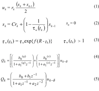
The model structure comprises two modules in series; the effective rain (loss) module given by Eqns. (1) to (3); and the UH module given by Eqn. (4), where the bracketed terms represent separate quick (q) and slow (s) response UHs acting in parallel. Equation (4) can be written as Eqn. (5), where the bracketed term represents a UH for total streamflow (the sum of quick and slow flow). Effective rainfall output from the loss module forms the input to the unit hydrograph module. Definitions of the symbols in Eqns. (1) to (5) are given in Table 1.
(
)
2 1 k-k k k s s r =u + (1)
( )
11
1
−
τ
−
+
k k w k ks
t
Cr
=
s
s0 = 0 (2))}
(
{
exp
)
(
t
k=
wf
R
-
t
kw
τ
τ
(3)(4)
(5)
Table 1. Definition of symbols
Symbol Definition
rk rainfall (mm) in timestep k (one day)
uk effective rainfall (mm)
sk catchment wetness index (dimensionless)
tk air temperature (oC)
τw catchment drying time constant (days) given by the value of τw(tk)
at reference temperature R (0°C in this paper)
f temperature modulation factor (°C-1)
C volume-forcing constant (mm-1) such that the volume of effective
rainfall matches that of observed streamflow over the model calibration period
Qk modelled streamflow (m3s-1)
b0(q) > 0 quick flow unit hydrograph parameters
–1< a1(q) < 1
b0(s) > 0 slow flow unit hydrograph parameters
–1 < a1(s) < 1
b0 , b1, a1, a2 parameters of the second-order transfer function expression of equation (4), where
b0= b0(q) + b 0
(s)
b1 = b0(q)a 1
(s) + b 0
(s) a 1
(q)
a1 = a1(q) + a 1
(s)
a2 = a1(q)a 1
(s)
z-n the backward shift operator such that z-nx
k = xk-n
δ pure time delay (days)
1
)
(
t
k<
wτ
δ − − − − + + + = k k u z a z a z b b Q 2 2 1 1 1 1 0 1 δ − − − + + += s k
The IHACRES methodology allows UH module structures other than the ‘two linear storages acting in parallel’ configuration represented by Eqns. (4) and (5), e.g. a single linear storage or two storages acting in series (Littlewood and Jakeman, 1994). For a large number of UK catchments analysed using daily data it can be shown that the ‘two in parallel’ configuration is a better representation of streamflow dynamics than either the ‘single storage’ or ‘two in series’ configuration. Therefore, given that an important stage in the formulation of a practical regionalisation scheme is the calibration of a common model structure to many catchments, the ‘two in parallel’ configuration is of considerable interest, particularly since it has the attractive physical interpretation of relatively quick and slow parallel flow pathways. It is reasonable to expect that the ‘two in parallel’ UH parameters (or dynamic response characteristics derived from the a and b parameters in Eqn. (4) as outlined below) will be related statistically to physical catchment attributes such as slope, drainage density and land-use, leading to estimation of UHs for non-gauged catchments. Indeed, this is the basis of regionalisation studies using IHACRES models (Sefton and Howarth, 1998; Post et al., 1998; Post and Jakeman, 1999)
For some catchments, however, or when the analysis is undertaken at a non-daily time step, a ‘two in parallel’ configuration in the UH module may not be optimal. Using daily data for an Australian catchment Young et al. (1997) found a ‘three storages in parallel’ configuration to be optimal, where the third storage represents a consequence of effective rainfall solely within the time step that the effective rainfall occurred (not additionally in subsequent time steps as for the other two storages). For a catchment in
which dominant quick and slow response streamflow components are clearly observable in a daily time series plot, the slow flow component parameters may not be reliably identifiable from a modelling analysis of monthly data; it may only be possible to estimate with useful precision the parameters of a ‘single storage’ UH module in such cases. It is tempting to believe that the finer the modelling data time step the more complex a configuration of linear storages in the UH module can be identified (i.e. the greater the number of parameters that can be estimated reliably). However, using six-minute interval data for a small catchment in China, Jakeman and Hornberger (1993) concluded that the ‘two in parallel’ configuration (having just three parameters as explained later) was the best that could be achieved in that case. The arguments for exploiting the ‘two in parallel’ UH module structure for regionalisation work, before trying to apply more complex configurations, are therefore very strong and this paper concentrates on that configuration in the UH module.
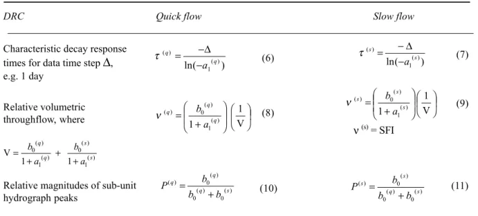
Dynamic response characteristics (DRCs) for dominant quick and slow response components of streamflow can be calculated from the a and b parameters in Eqn. (4), using Eqns. (6) to (11) in Table 2 (Jakeman et al., 1990; Littlewood and Jakeman, 1994). One of these DRCs, ν(s), is a Slow Flow
Index (SFI) analogous to the Base Flow Index (BFI, e.g. Gustard et al., 1989).
Using different loss modules to suit local hydroclimatological conditions, IHACRES with the ‘two in parallel’ UH configuration has been applied to many catchments to assist with different types of study: regionalisation for catchments in the United Kingdom (Sefton and Howarth, 1998) and Australia (Post et al., 1998;
Table 2. Unit hydrograph DRCs
DRC Quick flow Slow flow
Characteristic decay response times for data time step
∆
, e.g. 1 day) ( ln 1( ) ) ( q q a − ∆ − = τ ) ( ln 1() ) ( s s a − ∆ − = τ Relative volumetric throughflow, where ) ( 1 ) ( 0 ) ( 1 ) ( 0 1 1 V s s q q a b a b + + + = V 1 1 1()
) ( 0 ) ( + = s s s a b ν
ν(s) = SFI
Relative magnitudes of sub-unit hydrograph peaks ) ( 0 ) ( 0 ) ( 0 ) ( s q q q b b b P + = () 0 ) ( 0 ) ( 0 ) ( s q s s b b b P + = (6) (8) (10) (7) (9) (11) V 1 1 1( )
Post and Jakeman, 1999); semi-arid Australian catchments (Ye et al., 1997); environmental change impacts in selected catchments in the UK and North America (Jakeman et al., 1993a,b; Sefton and Boorman, 1997; Boorman and Sefton, 1997); and snow-affected catchments in Australia (Schreider et al., 1996, 1997) and Scotland (Steel et al., 1999). Furthermore, using either the loss module described by Eqns. (1) to (3), or a more process-oriented simple water balance loss module (Roberts and Harding, 1996), IHACRES has helped to address the issue of the level of parameterisation that can be justified in catchment-scale rainfall-runoff models identified solely from rainfall, streamflow and air temperature data (Jakeman and Hornberger, 1993; Littlewood, 2002a).
The Teifi at Glan Teifi has been employed previously as a bench-mark catchment to investigate practical aspects of UH model calibration and selection for continuous flow simulation (Littlewood, 2001, 2002b). The method of selecting a provisionally ‘best’ IHACRES model presented by Jakeman et al. (1990) and Littlewood and Jakeman (1994) involves a trade-off between a high Nash and Sutcliffe (1970) efficiency criterion (i.e. Dc, the proportion of variance in observed streamflow accounted for by the model) and, in recognition that unit hydrograph identification is a major modelling objective, a low ‘percentage average relative parameter error’ (%ARPE) for the unit hydrograph parameters (equations for Dc and ARPE are given in an Appendix). This paper continues to use the Teifi case study to investigate and improve upon the Dc – %ARPE trade-off model selection procedure. Two possible improvements to the procedure are tested: the application of a non-integer pure time delay, δ, in Eqns. (4) and (5) (PC-IHACRES v1.02 allows only integer values ofδ); and adjustment of one of the loss module parameter f in Eqn. (3) while searching for a good match between flow duration curves for observed and modelled flows.
The catchment and its data
The catchment of the Teifi to Glan Teifi drains an area of 894 km2 in south-west Wales and is underlain by impermeable Silurian and Ordovician bedrock. There are no substantial aquifers. Mean annual precipitation, 1959– 1995, was 1355 mm (mostly as rainfall but occasionally as snow) and mean annual runoff was 997 mm, or 73% of precipitation (Marsh and Lees, 1998). Population density for the whole Teifi river basin to Cardigan Bay (1012 km2) is just 37 km–2 (Environment Agency, 1997), and is largely concentrated in nine towns. The largest town, Cardigan, is downstream of Glan Teifi. Two small lakes (Llyn Egnant, 522,800 m3 and Llyn Teifi, 704,600 m3) and an area of
wetland (Tregaron Bog) affect streamflow dynamics in the upper catchment. At Glan Teifi, however, the flow regime is essentially unaffected by these headwater features or by contemporary anthropogenic factors. At catchment scale (to Glan Teifi) surface and near-surface hydrological processes are the dominant streamflow generation mechanisms.
A time series of daily areal rainfall for the catchment was derived by the method of Jones (1983), using point raingauge data. The number of raingauges in and close to the catchment available to calculate daily catchment rainfall varies with time, e.g. between 19 and 27 from 1980 to 1990 (Littlewood, 2001). The time series of Teifi daily mean river flows was obtained from the United Kingdom National River Flow Archive (Marsh and Lees, 1998). Unless stated otherwise, monthly air temperatures for square 135 in the MORECS scheme (Hough and Jones, 1997) were used for tk in Eqn. (3); daily values of tk in a particular month were assigned the appropriate monthly temperature. For the Teifi, and many other United Kingdom catchments, the effect of using monthly temperature with daily rainfall, rather than daily values for both, to model daily streamflow with IHACRES is only a small loss in model performance (sometimes hardly discernible).
Previous IHACRES models for the
Teifi
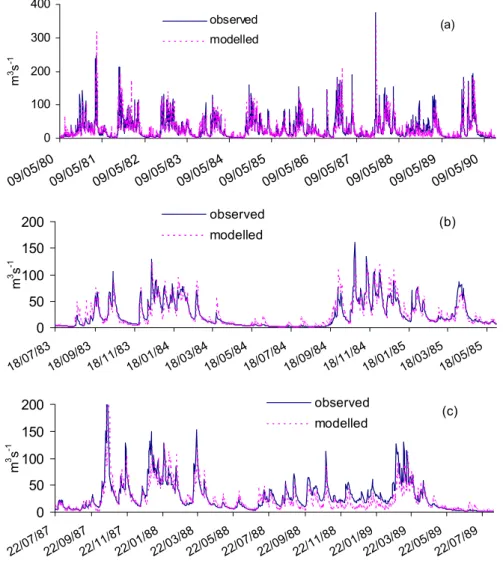
Previous papers have analysed the Teifi flow regime using IHACRES (Littlewood and Jakeman, 1991, 1992; Jakeman et al., 1993b) but the starting point for this paper is the set of results from an analysis of the daily flow record from 9th May 1980 to 14th August 1990 presented by Littlewood (2001). In that work the period was divided into eight, approximately three-year, overlapping, sub-periods designated #1, #2, …, #8. The whole period was designated #1–8. A ‘best’ Dc – %ARPE trade-off model calibrated over period #1 was called model #1, and so on. Models were calibrated over period #1-8, and each of the sub-periods, using a pure time delay, δ, in Eqns. (4) to (5) of one day, i.e. within PC-IHACRES v1.02 the rainfall record was shifted forward by one day prior to model calibration (better models were obtained with δ =1 day than with δ= 0 or δ= 2 days).
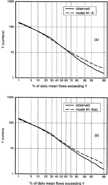
that either some of the data within that winter period are not of good quality or that, for reasons yet to be discovered, the model or modelling software is unable to cope with this sequence of observed data (this point is discussed again later). Figure 2a shows flow duration curves for observed and modelled flows (model #1–8) for period #1–8. (In order to minimise model warm-up effects, the first 20 days were excluded from all flow duration curve analyses presented in this paper.) Although model #1–8 accounts for 85% of the initial variance in observed streamflow over period #1– 8 (see Dc = 0.855 for model #1–8 in Table 3 where details of all the models referred to in this paper are given), Fig. 2a shows that, in percentage terms, model #1–8 performs much less well at low flows than at higher flows. Doubts concerning (a) the quality of the hydrometric data for winter 1988/89 and (b) the ability of the model or software to perform well over that period, led to subsequent model
calibrations in this paper being restricted to the period 9th May 1980 to 25th June 1988, i.e. period #1–6 according to the convention adopted by Littlewood (2001). Because the 1988/89 winter period was not used for its calibration, model #1–6(a) is better than model #1–8 in terms of its Dc and bias (mean observed minus mean modelled flow), as shown in Table 3, but it still performs poorly at low flows (Fig. 2b).
An attempt to improve model #1–6(a) was made in two stages. First, a non-integer pure time delay (0 < δ<1) was introduced by taking a portion x (0.1, 0.2, …, 0.9) of the rainfall on day i, and adding this amount to 1 – x of the rainfall on day i + 1. Second, loss module parameter f in Eqn. (3) was adjusted by trial and error in search of better model performance at low flows, using the match between flow duration curves for modelled and observed flows as an additional goodness-of-model-fit criterion.
0 100 200 300 400
09/05/8009/05/8109/05/8209/05/8309/05/8409/05/8509/05/8609/05/8709/05/8809/05/8909/05/90
m
3s
-1
observed modelled
(a)
0 50 100 150 200
18/07/8318/09/8318/11/8318/01/8418/03/8418/05/8418/07/8418/09/8418/11/8418/01/8518/03/8518/05/85
m
3 s
-1
observed
modelled
(b)
0 50 100 150 200
22/07/8722/09/8722/11/8722/01/8822/03/8822/05/8822/07/8822/09/8822/11/8822/01/8922/03/8922/05/8922/07/89
m
3 s
-1
observed
modelled (c)
Refining the Teifi model-fit
NON-INTEGER PURE TIME DELAY
Rainfall datasets were prepared for non-integer time delays δ of 0.1, 0.2, …, 0.9 days respectively and, keeping the analysis manageable by using the same loss module parameters as model #1-6(a) (i.e. τw = 22 days, f = 1.1), only the unit hydrograph module was recalibrated for each value of δ. The cases of δ = 0 and δ = 1 day were executed straightforwardly using the integer pure time delay facility of PC-IHACRES v1.02. Figure 3 shows the trade-off statistics Dc and %ARPE as δ varies between zero and one
day (a small value of %ARPE indicates good average
precision of the unit hydrograph parameters). The dashed lines in Fig. 3 indicate that when δ was0.1, 0.2, 0.3 and 0.4 days respectively the unit hydrograph a and b parameters in Eqn. (5) did not converge successfully during calibration (see below), or that they converged to physically unrealistic values represented, for example, by one or more negative DRCs according to Eqns. (6) to (11) in Table 2. A characteristic of the Simple Refined Instrumental Variable (SRIV) parameter identification algorithm (Young, 1985) used in IHACRES to estimate the UH parameters is that successful parameter convergence does not always occur in practice (for reasons too many and complex to be discussed here but see Jakeman et al., 1990) for a partial solution to this problem involving pre-filtering of system input and output prior to parameter identification). For the Teifi, by allowing loss module parameters other than τw = 22 days and f = 1.1oC–1, UH parameter convergence was successful for values of δ from 0.1 to 0.4 days (0.1 increments) butthis did not make appreciable changes to the position and shape of the Dc and %ARPE curves in Fig. 3. Therefore, on the basis of coincidental high Dc and low %ARPE, a time delay of 0.6 days was selected to give model #1–6(b) (but as can be noted in Fig. 3,the highest Dc and lowest %ARPE do not coincide exactly). In terms of Dc, bias and %ARPE, model #1–6(b) is better than model #1– 6(a) (see Table 3) but it still performs poorly at low flows; the flow duration curve for model #1-6(b) in Fig. 4shows that it tends to over-estimate flows smaller than the flow exceeded for about 40% of the time (the 40 percentile flow). Indeed, model #1–6(b) is only slightly better at low flows than model #1–6(a).
LOSS MODULE ADJUSTMENT
It was discovered that by varying loss module parameter f in Eqn. (3), while leaving δ and τw unchanged at 0.6 days and 22 days respectively, and re-calibrating the UH Fig. 2. Flow duration curves for (a) model #1-8, 29th May 1980
to 14th August 1990 and (b) model #1-6(a), 29th May 1980 to 25th June 1988
Fig. 3. Trade-off statistics Dc and %ARPE 0.84
0.86 0.88 0.9
0 0.2 0.4 0.6 0.8 1
Pure time delay (days)
0.010 0.012 0.014
%ARPE
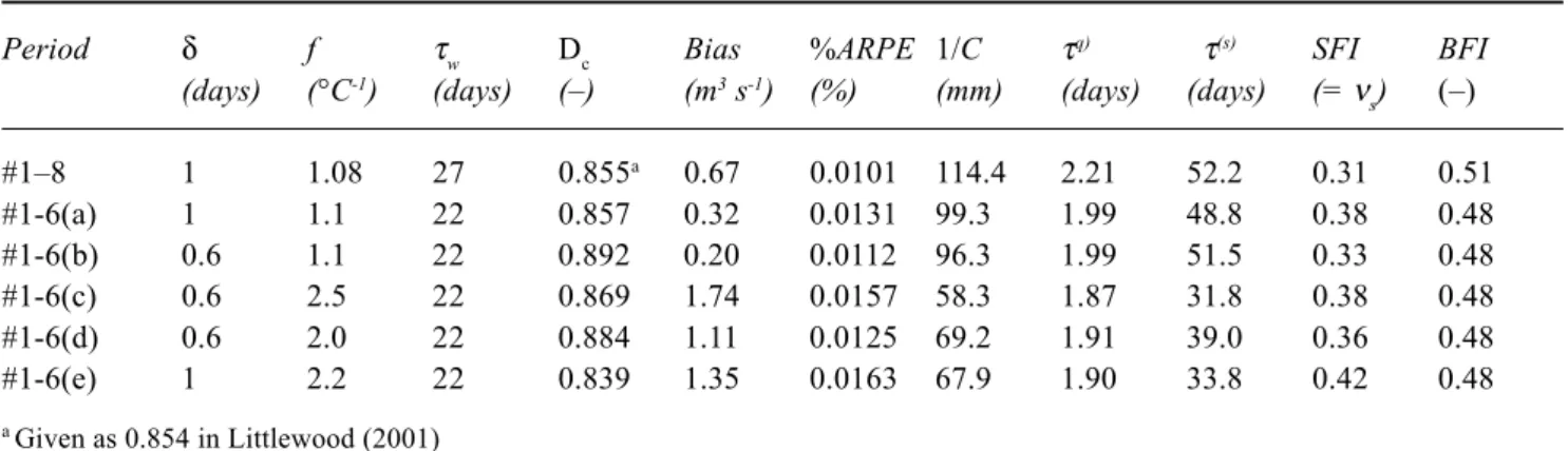
Table 3Calibration model-fit statistics and dynamic response characteristics (DRCs)
Period δ f τw Dc Bias %ARPE 1/C τq) τ(s) SFI BFI
(days) (°C-1) (days) (–) (m3 s-1) (%) (mm) (days) (days) (= ν
s) (–)
#1–8 1 1.08 27 0.855a 0.67 0.0101 114.4 2.21 52.2 0.31 0.51
#1-6(a) 1 1.1 22 0.857 0.32 0.0131 99.3 1.99 48.8 0.38 0.48
#1-6(b) 0.6 1.1 22 0.892 0.20 0.0112 96.3 1.99 51.5 0.33 0.48
#1-6(c) 0.6 2.5 22 0.869 1.74 0.0157 58.3 1.87 31.8 0.38 0.48
#1-6(d) 0.6 2.0 22 0.884 1.11 0.0125 69.2 1.91 39.0 0.36 0.48
#1-6(e) 1 2.2 22 0.839 1.35 0.0163 67.9 1.90 33.8 0.42 0.48
a Given as 0.854 in Littlewood (2001)
Fig. 4. Flow duration curves 29th May 1980 to 25th June 1988
parameters, the low-flow end of the flow duration curve for Teifi modelled flows could be better positioned, while leaving the good model-fit at high flows essentially unaffected. Figure 4 shows that model #1–6(c), with f = 2.5 oC–1, tends to under-estimate low flows whereas model #1-6(d), with f = 2.0oC–1, gives a flow duration curve that matches low observed flows more closely than any of the previous models, without appreciable change in model performance at higher flows.
In the previous sub-section, the introduction of a non-integer pure time delay δ of 0.6 days, while leaving τw = 22 days and f = 1.1 (oC-1), led to model #1–6(b) having only a slightly better model-fit (in terms of Dc) than model #1– 6(a). However, the relatively poor model-fit at low flows was not improved substantially. Changing model #1–6(d) by reverting to δ = 1 day and setting f = 2.2 oC–1 gives a flow duration curve for model #1–6(e) (not shown here) which is comparable over its 5 percentile to 95 percentile
range to that for model #1–6(d). Clearly, once a sub-optimal Dc – %ARPE trade-off model has been identified, it is the further adjustment of parameter f, not δ, which controls the better positioning of the lower end of the flow duration curve for modelled flows.
Uncertainty in the unit hydrograph
parameters
The SRIV unit hydrograph parameter identification algorithm yields standard errors for the UH a and b parameters in Eqn. (5) (Jakeman et al., 1990). For each model referred to above, Table 4 shows the UH DRCs with their indicative precisions. The precision associated with a DRC, given in parentheses in Table 4 as lower and upper 95% confidence limits expressed as percentage departures from the stated DRC value, was derived automatically. The software takes 1000 random samples from normal distributions defined by the best estimates of the a and b parameters in Eqn. (5) and their standard errors. Equations (6) to (11) are then applied to each sample, the results for each DRC ranked, and appropriate percentiles selected by the software.
Inspection of Table 4 shows that for each type of DRC (τ, ν or P), and each model, the normalised (%) precision associated with the slow flow DRC is greater than that for the quick flow DRC. It can be recalled (see Figs. 2 and 4)
Discussion
GOOD ESTIMATION OF τ(S) – THE KEY TO
MODELLING LOW FLOWS
Comparing models #1–6(a) and #1–6(d), the difference in the quick flow DRCs is fairly modest (Table 4): (τ(q)
decreases from 1.99 to 1.91 days (– 4%); ν(q) decreases by
two percentage points, from 38% to 36%; and P(q) decreases
by only 0.4 of one percentage point, from 97.0% to 96.6%. By definition ν(q) +ν(s) = 1 and P(q) + P(s) = 1, so the changes
in slow flow DRCs ν(s) and P(s) are also modest. The change in τ(s), however, is substantial, decreasing from 48.8 days to
38.9 days (– 20%), indicating the importance of being able to estimate τ(s) accurately (i.e.without bias) in order to model
low flows well.
In catchments like the Teifi, where surface and near-surface hydrological processes largely control streamflow event responses, the DRC precisions in Table 4 indicate that, as might be expected, it is more difficult to identify the dominant slow flow component than the quick. In catchments where deeper (slower) flow pathways are dominant it is likely to be the quick response component that is more difficult to identify.
REGIONALISATION
The Teifi at Glan Teifi is one of 60 catchments for which
the IHACRES model defined by Eqns. (1) to (4) was calibrated on the basis of a trade-off between Dc and %ARPE, to assist with UK regionalisation and climate change impact studies (Sefton and Howarth, 1998; Sefton and Boorman, 1997; Boorman and Sefton, 1997). As discussed elsewhere (Littlewood, 2002d), inspection of the Teifi model parameters used in those studies (Sefton, pers. comm.) reveals that that model also over-estimates low flows. The extent to which IHACRES models for other catchments employed in the studies by Sefton and Howarth (1998) and Sefton and Boorman, (1997) might have been inaccurate (i.e. biased) at low flows has yet to be established. However, work in progress by the author (not discussed in detail here but intended for publication) indicates that for six other catchments in Wales, four of which were employed in the regionalisation studies referred to, five exhibit a similar systematic over-estimation of low flows when a ‘best’ model is selected according to a trade-off between a high Dc and a low %ARPE without using other model-fit criteria. Furthermore, for four of those five catchments the lower end of the flow duration curve can be re-positioned to give a good match with that for observed low flows, simply by adjusting parameter f in the way that has been described in this paper. It appears, therefore, that at least some of the 60 τ(s) values used in the previously mentioned regionalisation studies were sub-optimal. This may help to Table 4. Unit hydrograph DRCs with 95% confidence level uncertainties (expressed as percentage departures from the stated value)
model τ(q) τ(s) ν(q) ν(s) P(q) P(s)
(days) (days)
#1-8 2.21 52.2 0.687 0.313 0.977 0.023
(-4.1 +4.1) (-13.0 +17.8) (-2.6 +2.6) (-5.7 +5.7) (-0.4 +0.4) (-16.8 +17.2)
#1-6(a) 1.99 48.8 0.623 0.377 0.970 0.030
(-4.5 +5.0) (-11.6 +15.2) (-2.7 +2.9) (-5.0 +4.5) (-0.5+0.4) (-15.2 +15.
#1-6(b) 1.99 51.5 0.667 0.333 0.976 0.024
(-4.0 +4.5) (-11.4 +14.4) (-2.4 +3.0) (-5.4 +4.8) (-0.3 +0.3) (-13.9 +14.7)
#1-6(c) 1.87 31.8 0.616 0.384 0.955 0.045
(-5.3 +4.8) (-11.3 +13.5) (-3.1 +3.2) (-5.2 +4.9) (-0.7 +0.7) (-14.4 +15.7)
#1-6(d) 1.91 38.9 0.637 0.363 0.966 0.034
(-4.2 +4.7) (-10.0 +14.1) (-2.7 +2.8) (-5.2 +4.7) (-0.5 +0.5) (-14.9 +13.4)
#1-6(e) 1.90 33.8 0.576 0.424 0.950 0.050
(-5.3 +5.8) (-10.9 +14.8) (-3.4 +4.2) (-5.7 +4.7) (-0.7 +0.8) (-15.6 +14.2)
Notes: ν(q) + ν(s) = 1
explain the poor-quality τ(s) regionalisation equation (coefficient of correlation = 0.37) reported by Sefton and Howarth (1998) relative to that for other regression equations (0.41 to 0.80) that the authors presented for linking other DRCs to physical catchment descriptors (PCDs) (see Table 5). An additional reason why the IHACRES model for the Teifi calibrated for that work was sub-optimal is given in the last paragraph of the next section.
since they are simplistic” (Boorman and Sefton, 1997). The authors went on to say that it follows that the J–H loss module is therefore not suitable for climate change scenario studies. While this may be strictly correct it is worth noting that the climate change scenarios applied by these authors were also simplistic, comprising prescribed, month-by-month, changes in temperature and rainfall on a repetitive basis for consecutive years, according to outputs from global circulation model (GCM) experiments. If such GCM indications of how the climate might change are expressed in long, synthetic but realistic, time series of temperature and rainfall for simulating streamflow under a changed climate, then IHACRES will not give the same percentage change in streamflow for all catchments in response to a given percentage change in rainfall. Furthermore, provided that the prescribed mean changes in rainfall and temperature in such synthetic data sequences were not large it is believed that IHACRES incorporating the J–H loss module would give a useful indication of the impact of climate change scenarios on flow regimes. Nevertheless, a loss module that behaves with more hydrological integrity for assessing climate change impacts is required. The J–H loss module was not developed with that application uppermost in mind but it is an efficient and very useful parameterisation of the catchment-scale rainfall–effective rainfall process for many purposes, as demonstrated in this paper.
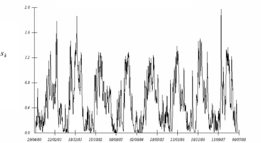
Turning now to the matter of the catchment wetness index, sk, generated by the J–H loss module, Fig. 5 shows the sequence of sk for Teifi model #1-6(d) over its calibration period (9th May 1980 to 25th June 1988). The temporal pattern in Fig. 5 is, as required, seasonal but it exhibits features that are not wholly satisfactory in a hydrological sense. If, simplistically, sk = 1 is considered to correspond to the situation when the entire catchment is contributing to streamflow (sk = 0 corresponding to a zero contributing area) then values of sk greater than unity (during every winter in Fig. 5) do not tally with the variable contributing area concept of how catchments respond dynamically to generate streamflow (e.g. Robinson, 1993). The contributing area, expressed as a fraction of the catchment area, cannot, of course, be greater than unity. On the basis of the variable contributing area concept, one would not expect sk to plummet to zero or near-zero every summer, as it does in Fig. 5,while during wet periods (especially in winter) one would expect sk to approach unity asymptotically (sk = 1 representing wetness conditions associated with an almost inconceivably large flood and therefore extremely unlikely to occur for a catchment the size of the Teifi to Glan Teifi). Although the J–H loss module is demonstrably successful within the IHACRES framework for many purposes, process-oriented hydrologists might prefer a loss module Table 5.Correlation coefficients for DRC-PCD multiple
regression regionalisation equations
DRC f τw C-1 τ(q) τ(s) ν(s)
r 0.80 0.41 0.61 0.64 0.37 0.77
Source: Sefton and Howarth (1998)
A CRITIQUE OF THE LOSS MODULE
The work presented in this paper does not mark the end-point in a search for a best loss module for inclusion within robust IHACRES software for rainfall-streamflow modelling to assist with regionalisation and other studies. The following three points need attention before the approach can be applied systematically for such studies with greater confidence. First, Boorman and Sefton (1997) noted that, irrespective of the catchment in question, for a given percentage increase in rainfall the loss module given by Eqns. (1) to (3), which was introduced by Jakeman and Hornberger (1993) and is referred to subsequently here as the J–H loss module, predicts a constant percentage increase in effective rainfall. The J–H loss module is not suitable, therefore, for climate change sensitivity analyses. Second, the simulation of catchment wetness index (sk in Eqn. 2 given earlier in this paper) does not always give an entirely reasonable sequence for such an index. Third, although an IHACRES model can simulate streamflow well over long periods, sequences within the Teifi record have been noted when such a model performs poorly (e.g. Fig. 1c). Each of these points is now discussed in more detail.
that is structured and which behaves internally more in line with their observations of how water moves in catchments. Evans and Jakeman (1998) developed an alternative loss module of this type for application in an IHACRES framework, applying it to two catchments in the United States and one in Australia, but it has yet to be assessed for systematic application to catchments in Wales and elsewhere in the United Kingdom. Similarly, Littlewood (2002a) successfully applied the Roberts and Harding (1996) conceptual soil-vegetation-atmosphere transfer (SVAT) module in series with the IHACRES unit hydrograph module to a small Kenyan catchment dominated by bamboo vegetation, for which land-use the SVAT module had been calibrated using soil moisture measurements. Although for the Kenyan catchment in question the SVAT module performed better than the J-H loss module, with the ‘two in
parallel’ configured UH, its utility in rainfall–streamflow models for other catchments (with different parameters) has yet to be tested.
The third issue was mentioned earlier in the paper with reference to Fig. 1c, which shows the poor performance of model #1–8(a) over the 1988/89 winter period for the Teifi. Checks indicated that this inadequate performance is not due to poor data or to a poorly parameterised model; the sequences of Teifi rainfall and streamflow for 1988 and 1989 compare favourably with those for other catchments in the region; and model #1–6(d), i.e. the improved model for the Teifi identified in this paper, also performs poorly over the winter period 1988/89 (Fig. 6). It appears, therefore, that either (a) there is an error in the PC-IHACRES v1.02 software package, or (b) the IHACRES model cannot cope with such winter sequences where the hydrograph comprises sk
Fig. 5. Model #1-6(d) catchment wetness index, sk , 9
th May 1980 to 25th June 1988
Fig. 6. Model #1-6(d) simulation 22nd July 1987 – 9th August 1989 0
50 100 150 200
22/07/8722/09/8722/11/8722/01/8822/03/8822/05/8822/07/8822/09/8822/11/8822/01/8922/03/8922/05/8922/07/89
m
3s
-1
observed
many relatively small events, or (c) both (a) and (b) apply in different measures (but this seems unlikely). If the IHACRES model cannot cope (option (b) above) it could be because of a problem in the J–H loss module.
The author has noted other winter periods for the Teifi (and similar sub-periods for other catchments in the region) that exhibit the same hydrograph characteristics to those shown for 1988/89 in Fig. 6, where an IHACRES model performs poorly despite its good performance at other times. Further work is necessary to solve this problem and until it is resolved the analyst should proceed with caution when such sub-periods of record are involved. It is unfortunate, therefore, that the regionalisation study referred to previously used data from years 1986 to 1989 to calibrate IHACRES models; for the Teifi the period 6th October 1986 to 24th July 1989 was used (Sefton, pers. comm.). The IHACRES software used for the studies by Sefton and Howarth (1998) and Sefton and Boorman (1997) also exhibits poor model performance over the 1988/89 winter period and during other similar sequences of streamflow in the Teifi record, suggesting that the problem is not specific to the PC-IHACRES v1.02 package. With the benefit of hindsight informed by careful hydrological validation of modelled streamflow it appears, therefore, that there are two reasons why the models for the Teifi and probably other catchments were sub-optimal in the regionalisation studies referred to previously in this paper: systematic over-estimation of τ(s); and an unfortunate choice of period for calibrating the models.
Concluding remarks
Flow duration curves have been used as an effective additional model-fit criterion to the Dc – %ARPE trade-off recommended previously, leading to a greatly improved IHACRES model for the Teifi at Glan Teifi at low flows. While model-fit statistics (e.g. Dc and %ARPE) undoubtedly form a good basis on which to select a preliminary ‘best’ model, especially when used in combination, the utility of the additional use of flow duration curves for ensuring that a model performs well over a wide range of flows has been demonstrated. Indeed, the author would strongly recommend that comparisons of log-normal flow duration curves for observed and modelled flows, as shown in Figs. 2 and 4 of this paper, form an integral part of all rainfall – streamflow modelling studies.
The model selection procedure developed here is a blend of (a) using a trade-off of model-fit statistics calculated automatically by the modelling software and (b) subsequent manual intervention based on trial-and-error manipulation of loss module temperature modulation parameter f in search
of an improved match between (low) flow duration curves. It is an example, therefore, of combining the strengths of automatic and manual model calibration approaches (Boyle et al., 2000) which is becoming increasingly recognised as an important and necessary feature of the toolkit approach to rainfall–streamflow modelling (e.g. Wagener et al., 2001). The log-normal flow duration curve is a tool of long-standing use by hydrologists and, as has been demonstrated here, deserves to be included as a standard element of rainfall–streamflow modelling packages and toolboxes.
Bias in the estimation of Teifi low flows has been substantially reduced using an improved model selection procedure. By this means an IHACRES model with just six parameters (model #1-6(d)) has been identified that characterises very well the flow regime at Glan Teifi over its 5 percentile to 95 percentile range (model #1–6(d) in Fig. 4). Flows between the 1 percentile and the 5 percentile (and between the 95 percentile and the 99 percentile) are modelled reasonably well, bearing in mind the inherent instability of these sections of duration curves for observed flows.
A major improvement of the unit hydrograph characterisation of low flows for the Teifi has been achieved which has important implications for regionalisation studies. The extent to which the IHACRES models calibrated for the Sefton and Howarth (1998) regionalisation study exhibit systematic error at low flows has yet to be established. Until this matter is resolved, that regionalisation scheme should be treated with caution, especially where low flows are the primary interest. The work presented in this paper allows speculation that it will be possible to improve upon the set of τ(s) values that can be made available to assist with
regionalisation of UK low flows.
The rainfall-streamflow model is but one stage in the regionalisation process during which systematic errors can be introduced. Littlewood (2002c) describes how bias can be introduced when a regionalisation equation linking DRCs and physical catchment descriptors (PCDs) is the back-transformation of a regression model that was derived using logarithms of the variables.
Acknowledgements
The author thanks Catherine Sefton for information about how IHACRES was applied for regionalisation and for details of individual models calibrated for that work. Thanks are due also to two anonymous reviewers for their helpful and constructive comments on an earlier draft of the paper.
References
Beven, K.J., 2000. Rainfall-Runoff Modelling: The Primer. Wiley, Chichester, UK. 360pp.
Boorman, D.B. and Sefton, C.E.M., 1997. Recognising the uncertainty in the quantification of the effects of climate change on hydrological response. Climatic Change, 35, 415–434. Boyle, D.P., Gupta, H.V. and Sorooshian, S., 2000. Toward
improved calibration of hydrologic models: combining the strengths of manual and automatic methods. Water Resour. Res.,
36, 3663–3674.
Environment Agency, 1997. Catchment management plan; Teifi action plan. Environment Agency for England and Wales, UK. 21pp.
Evans, J.P. and Jakeman, A.J., 1998. Development of a simple, catchment-scale, rainfall-evapotranspiration-runoff model.
Environ. Model. Software, 13, 385–393.
Gustard, A., Roald, L. A., Demuth, S., Lumadjeng, H. S. and Goss, R., 1989. Flow Regimes from Experimental and Network Data (FRIEND), vol. I, Hydrological Studies. Institute of Hydrology, Wallingford, Oxfordshire, UK.
Hough, M.N. and Jones, R.J.A., 1997. The United Kingdom Meteorological Office rainfall and evaporation calculation system: MORECS version 2.0 – an overview. Hydrol. Earth Syst. Sci., 1, 227–239.
Jakeman, A.J. and Hornberger, G.M., 1993. How much complexity is warranted in a rainfall-runoff model? Water Resour. Res., 29, 2637–2649.
Jakeman, A.J., Littlewood, I.G. and Whitehead, P.G., 1990. Computation of the instantaneous unit hydrograph and identifiable component flows with application to two small upland catchments. J.Hydrol., 117, 275–300.
Jakeman, A.J., Littlewood, I.G. and Whitehead, P.G., 1993a. An assessment of the dynamic response characteristics of streamflow in the Balquhidder catchments. J. Hydrol., 145, 337– 355.
Jakeman, A.J., Chen, T.H., Post, D.A., Hornberger, G.M., Littlewood, I.G. and Whitehead, P.G., 1993b. Assessing uncertainties in hydrological response to climate change at large scale. In: Macroscale Modelling of the Hydrosphere, W.B. Wilkinson (Ed.), Proc. of the Yokohama Symposium, July 1993,
IAHS Publication no. 214, 37–47.
Jones, S.B., 1983. The estimation of catchment average point rainfall profiles. IH Report No. 87, Institute of Hydrology, Wallingford, UK.
Littlewood, I.G., 2001. Practical aspects of calibrating and selecting unit hydrograph-based models for continuous river flow simulation. Hydrol. Sci. J., 46, 795–811.
Littlewood, I.G., 2002a. Sequential conceptual simplification of the effective rainfall component of a rainfall-streamflow model for a small Kenyan catchment. In: Proc. International Environmental Modelling and Software Society Conference, Vol. I, A.E. Rizzoli and A.J. Jakeman (Eds.). 24–27 June, 2002, Lugano, Switzerland, 422–427.
Littlewood, I.G., 2002b. Unit hydrograph characterisation of continuous quick and slow response components of river flow: applications and uncertainties. In: Continuous river flow simulation: methods, applications and uncertainties, I.G. Littlewood (Ed.). British Hydrological Society Occasional Paper No. 13, 1–9.
Littlewood, I.G., 2002c. A source of bias in regionalisation equations. Circulation, Newsletter of the British Hydrological Society, No. 72, 9–11.
Littlewood, I.G., 2002d. An improved procedure for identifying quick and slow response unit hydrographs for regionalisation of high and low flows. Proc. British Hydrological Society, 8th
National Hydrology Symposium, University of Birmingham, 8-11 September 2002, 121–126.
Littlewood, I.G. and Jakeman, A.J., 1991. Hydrograph separation into dominant quick and slow flow components. Proc. Third National Hydrology Symposium, British Hydrological Society, 3.9–3.16.
Littlewood, I.G. and Jakeman, A.J., 1992. Characterisation of quick and slow streamflow components by unit hydrographs for single- and multi-basin studies. In: Proc. Fourth General Assembly of the European Network of Experimental and Representative Basins, Oxford, September 29 - October 2, M. Robinson (Ed.), published as IH Report 120, Institute of Hydrology, Wallingford, UK.
Littlewood, I.G. and Jakeman, A.J., 1994. A new method of rainfall-runoff modelling and its applications in catchment hydrology. In: Environmental Modelling (Volume II), P. Zannetti (Ed.). Computational Mechanics Publications, Southampton, UK, 143–171.
Littlewood, I.G., Down, K., Parker, J.R. and Post, D.A., 1997.
The PC version of IHACRES for catchment-scale rainfall-streamflow modelling: User Guide. Institute of Hydrology, Wallingford, UK. 97pp.
Marsh, T.J. and Lees, M.L. (Eds.), 1998. Hydrological data UK: Hydrometric Register and Statistics 1991-1995. Institute of Hydrology/British Geological Survey, Wallingford, UK. 207pp. Nash, J.E. and Sutcliffe, J.V., 1970. River flow forecasting through conceptual models. Part 1 — A discussion of principles. J. Hyrol., 27, 282–290.
Post, D.A. and Jakeman, A.J., 1999. Predicting the daily streamflow of ungauged catchments in S.E. Australia by regionalising the parameters of a lumped conceptual rainfall-runoff model. Ecol. Model., 123, 91–104.
Post, D.A., Jones, J.A. and Grant, G.E., 1998. An improved methodology for predicting the daily hydrologic response of ungauged catchments. Environ. Model. Software, 13, 395–403. Roberts, G. and Harding, R.J., 1996. The use of simple process-based models in the estimation of water balances for mixed land use catchments in East Africa. J. Hydrol., 180, 251–266. Robinson, M. (Ed.)., 1993. Inventory of streamflow generation
studies. Flow Regimes from International Experimental and Network Data (FRIEND), Vol III, Institute of Hydrology, Wallingford, UK. 73pp.
Schreider, S., Yu, W., Jakeman, A.J., Whetton, P.H. and Pittock, A.B., 1996. Estimation of climate impact on water availability and extreme events for snow-free and snow-affected catchments in the Murray-Darling basin. Aust. J. Water Resour., 2, 1–-13. Schreider, S., Yu, W., Whetton, P.H., Jakeman, A.J. and Pittock, A.B., 1997. Runoff modelling for snow-affected catchments in the Australian alpine region, eastern Victoria. J. Hydrol., 200, 1–23.
Sefton, C.E.M. and Howarth, S.M., 1998. Relationships between dynamic response characteristics and physical descriptors of catchments in England and Wales. J. Hydrol., 211, 1–16. Steel, M.E., Black, A.R., Werritty, A. and Littlewood, I.G., 1999.
Re-assessment of flood risk for Scottish rivers using synthetic runoff data. Proc. XXII General Assembly of the International Union of Geodesy and Geophysics, Birmingham, UK, 18–30 July 1999.
Wagener, T., Boyle, D.P., Lees, M.J., Wheater, H.S., Gupta, H.V. and Sorooshian, S., 2001. A framework for development and application of hydrological models. Hydrol. Earth Syst. Sci., 5, 13–26.
Wheater, H.S., Jakeman, A.J. and Beven, K.J., 1993. Progress and directions in rainfall-runoff modelling. In: Modelling change in environmental systems, A.J. Jakeman, M.B. Beck and M.J. McAleer (Eds.). Wiley, Chichester, UK. 101–132.
Ye, W., Bates, B. C., Viney, N. R., Sivapalan, M. and Jakeman, A. J., 1997. Performance of conceptual rainfall–runoff models in low-yielding ephemeral catchments. Water Resour. Res.33, 153– 166.
Young, P.C., 1985. The instrumental variable method: a practical approach to identification and system parameter estimation. In:
Identification and System Parameter Estimation 1985, Vols 1 and 2, H.A Barker and P.C. Young (Eds.). Pergamon, Oxford, UK. 1–16.
Young, P.C., Jakeman, A.J. and Post, D.A., 1997. Recent advances in the data-based modelling and analysis of hydrological systems. Water Sci.Technol., 36, 99–116.
Appendix
The coefficient of determination, Dc, is the proportion of initial variance in observed streamflow accounted for by the model. Dc is given by Eqn. (A1) where σ denotes standard deviation, and ξ and y denotemodel residuals and observed streamflow respectively.
2 2 1 c D ∧ ∧ − = y σ ξ σ (A1)
Referring to Eqn. (5), ARPE for a ‘two in parallel’ UH module is given by equation (A2). Jakeman et al. (1990) give a general equation for ARPE.
2 0 2 2 2 1
ARPE 1 2 0
+ ∧ ∧ + ∧ ∧ + ∧ ∧ = b b a a a
a σ σ