Journal of Applied Fluid Mechanics, Vol. 9, No. 4, pp. 1829-1837, 2016. Available online at www.jafmonline.net, ISSN 1735-3572, EISSN 1735-3645.
Numerical Prediction of Unsteady Behavior of Cavitating
Flow on Hydrofoils using Bubble Dynamics Cavitation
Model
N. Mostafa
1, M. M. Karim
2†and M. M. A. Sarker
31Department of Mathematics, Military Institute of Science and Technology, Dhaka-1216, Bangladesh 2Departmentof Naval Architecture and Marine Engineering, BUET, Dhaka-1000, Bangladesh
3Department of Mathematics, BUET, Dhaka-1000, Bangladesh
†Corresponding Author Email: [email protected]
(Received August 24, 2013; accepted July 4, 2015)
ABSTRACT
This paper presents a numerical study with pressure-based finite volume method for prediction of non-cavitating and time dependent non-cavitating flow on hydrofoil. The phenomenon of cavitation is modeled through a mixture model. For the numerical simulation of cavitating flow, a bubble dynamics cavitation model is used to investigate the unsteady behavior of cavitating flow and describe the generation and evaporation of vapor phase. The non-cavitating study focuses on choosing mesh size and the influence of the turbulence model. Three turbulence models such as Spalart-Allmaras, Shear Stress Turbulence (SST) k-ω model and Re-Normalization Group (RNG) k-ε model with enhanced wall treatment are used to capture the turbulent boundary layer on the hydrofoil surface. The cavitating study presents an unsteady behavior of the partial cavity attached to the foil at different time steps for σ=0.8. Moreover, this study focuses on cavitation inception, the shape and general behavior of sheet cavitation, lift and drag forces for different cavitation numbers. Finally, the flow pattern and hydrodynamic characteristics are also studied at different angles of attack.
Keywords: Cavitation; CAV2003 hydrofoil; Finite volume method; Turbulence model; Unsteady flow.
NOMENCLATURE
CD drag coefficient
CF frictional coefficient
CL lift coefficient
Cp pressure coefficient C1ε turbulence constant
Ce empirical constant c chord length fg gas mass fraction
fv vapor mass fraction
p pressure pv vapor pressure
p∞ system pressure Re vapor generation source term
Rc vapor condensation source term
α volume fraction vector differential operator
μt turbulent viscosity
turbulent kinematic viscosityγ surface tension density l liquid density
m mixture density
σ cavitation number
ε turbulent dissipation rate
1.
INTRODUCTION
Cavitation in hydraulic machines causes different problems like vibration, increase in hydrodynamic drag, pressure pulsation, and change in flow kinematics, noise and erosion of solid surface. Most of these problems are related to transient behavior of cavitation structure. Cavitation erosion is
investigate cavitation phenomena and validate numerical procedures, a number of investigations were performed in the past by Kubota et al. (1992), Alajbegovic et al. (1999), Stutz et al. (2000), Schnerr et al. (2001), and Frobenius et al. (2003).In the last decade various methods for numerical simulation of cavitating flow were developed. Most of the studies treat the two phase flow as a single vapor-liquid phase mixture flow. The evaporation and condensation can be modeled with different source terms which are usually derived from the Rayleigh-Plesset bubble dynamics equation. Recently, Singhal et al. (2002) and different authors have proposed to consider a transport equation model for the void ratio, with vaporization/condensation source terms to control the mass transfer between two phases. This method has the advantage of taking into account the time influence on the mass transfer phenomena through empirical laws for the source term. It also avoids using quantities like bubble number density and initial bubble diameter. A cavitation model, based on bubble dynamics equation is used for computation of cavitating flows. Bubbles may appear in regions of low pressure. These bubbles are carried along by the flow and disappear when they enter into a region of higher pressure as described by Brennen (1995).The other way to model cavitation process is by the so called barotropic state law that links the density of vapor-liquid mixture to the local static pressure. The model was proposed by Delannoy and Kueny (1990).
The influences of mesh and turbulence model in non-cavitating condition are studied previously by comparing the values of lift and drag by Mostafa (2009) and Karim et al. (2010).In this study,two cavitating conditions are separately analyzed, i.e., σ=0.8 where an unsteady partial cavitating behavior is obtained and σ=0.4 where a super cavitating flow is observed. Cavitating flows at different cavitation numbers are analyzed and an unsteady partial cavitating behavior at σ=0.8 is presented at different time steps. Finally, the hydrodynamic characteristics and flow pattern are also studied at different angles of attack.
2.
NUMERICAL SIMULATION
The numerical model uses an implicit finite volume method associated with multiphase and cavitation models. For numerical simulation of cavitating flow, a bubble dynamics cavitation model is used to describe the cavity formation. The RNG (Re-Normalization Group) k-ε turbulence model with enhanced wall treatment is used to capture boundary layer. The Reynolds number .9 × based on chord length is used. The corresponding is 5-15. A second order central scheme is used for discretization of space except the convective terms. The convective term in the momentum equation is discretized by the QUICK (Quadratic Upstream Interpolation Convective Kinetics) scheme for non cavitating flow where second order implicit scheme is used for cavitating problem. Pressure based solver
SIMPLE (Semi-Implicit Method for Pressure-Linked Equations) is used as the velocity pressure–coupling algorithm by Mostafa (2009).
3.
MULTIPHASE MODEL
A single fluid (mixture model) approach is used. Fluid density (which is the function of the vapor mass fraction fv) is computed from the mass and momentum conservation equations together with the transport equation and the equation of the turbulence model. The relation between mixture density(m) and vapor mass fraction(fv)was obtained by Dular et al. (2005) as:
1
1 v v
m v l
f f
(1)
The volume fraction of the vapor phase is related to the mass fraction of the vapor phase as:
v m v
v f
(2)
The mass conservation equation for the mixtureis given by
.
0 m m m v t
(3)
The momentum conservation equation for the mixture is given by:
v v
g Fp v v v t m T m m m m m m m m . .
(4)
And the transport equation for the vaporis given by:
mfv
mvmfv
Re Rct
. (5)
4.
CAVITATION MODEL
In cavitating condition, it is assumed that there are plenty of nuclei for the inception of cavitation. Thus a bubble dynamic equation is used for proper account of bubble growth and collapse. The bubble dynamic equation can be derived from the Rayleigh-Plesset equation as described by Singhal et al. (2002).
Finally, the working fluid is assumed as mixture of liquid, liquid vapor and no condensable gas. The Source terms Re and Rcare defined as vapor generation (liquid evaporation) and vapor condensation respectively. These source terms can be expressed as (Dular et al., 2005):
v g
l v v l e
e f f
p p k
C
R 1
3 2
(6)
v l v l l c c f p p k C R 3 2 (7)
whenppv
where and are empirical constants, and k isthe local kinetic energy, γ is surface tension, is vapor mass fraction and is mass fraction of non condensable(dissolve) gases. Values of and
are taken as 0.02 and 0.01 respectively.
5.
GEOMETRY
AND
COMPUTATIONAL DOMAIN
The section of the hydrofoil is presented in Fig. 1 which shows a schematic view of the CAV2003 hydrofoil geometry. The hydrofoil is placed at an angle of attack of7°. The equationof the upper surface of the symmetric foil geometry can be expressed as: ) 8 ( 4 4 3 3 2 2 1 0 c x a c x a c x a c x a c x a c y
where, a0=0.11858, a1=-0.02972, a2= 0.00593, a3= -0.07272, a4 = -0.002207
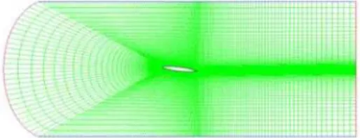
c is chord length,yy cand xx cis the dimensionless coordinate along the chord line. The flow field around the hydrofoil is modeled in two dimensions. The flow from left to right with the hydrofoil of chord length c=0.1m submersed in an incompressible fluid is considered. The hydrofoil is located at the middle of a channel of length 10c and height 4c. Fig. 1 shows the 2D computational domain and boundary conditions. The inlet boundary condition is specifiedas velocity inlet with a constant velocity profile which is 6 m/s. Upper and lower boundaries are slip walls, i.e., symmetry boundary condition. The outlet uses a constant pressure boundary condition. The foil itself is a no-slip wall, i.e., u = 0, v = 0 at the foil surface. A typical grid is shown in Fig. 2. Most of the cells are located around the foil and contraction of the grid is applied in its upstream part to obtain an especially fine discretization of the areas where cavitation is expected.
Fig. 1. Schematic diagram of the flow field around a CAV2003 hydrofoil with boundary
condition.
Fig. 2. The overall view of grid lines in mesh.
6.
INFLUENCE OF TURBULENCE
MODEL
To simulate non cavitating flow, there is a great influence of different turbulence models. Here, we simulate the non-cavitating flow with different turbulence models such as RNG k-ε with enhanced wall treatment, Spalart- Allmaras and the k-ω Shear Stress Turbulence model. The comparison among the different models is made on the basis of the predicted values of lift and drag coefficients as shown in Table 1and Table 2 in which the viscous and pressure parts are analyzed separately. The results show a good agreement with Spalart-Allmaras and k-ε with enhanced wall treatment. The k-ω model predicts lo w e r valuesw ith re sp e c t to other models . The differences are due to the calculation of a separated flow near the trailing edge.
In Table 3, computed lift and drag coefficient for the non cavitating flow with k-ε turbulence model is compared with the results of Pouffary et al. (2003) and
Table 1 Turbulence effect on lift
Models Lift coefficient Viscous Pressure Total k- ω -0.0005 0.5994 0.5989 Spalart-Allmaras -0.0004 0.6522 0.6518 k-ε with enhanced
wall treatment -0.0004 0.6567 0.6564
Table 2 Turbulence effect on drag
Models Drag coefficient Viscous Pressure Total k- ω 0.01061 0.01061 0.0212 Spalart-Allmaras 0.00886 0.02223 0.331 k-ε with enhanced
wall treatment 0.01013 0.01433 0.0245
Table 3 Comparison of and for non cavitating case
Present 0.656 0.0245
Pouffary 0.622 0.0294
Courtier-Delgosha 0.660 0.0150
Courtier-Delgosha et al. (2003) and k-ω model with Kawamura et al. (2003). The present result shows a good agreement on the prediction of the total lift especially with Courtier-Delgosha et al. (2003). Finally, we decided to use the k-ε model with enhanced wall treatment for cavitating calculations.
7. CAVITATING ANALYSIS
This section presents results computed for the typical cavitation numbers σ=0.8 and σ=0.4. For simulation the convergence criterion is determined by observing the evaluation of different flow parameters (velocity magnitude at inlet, static pressure behind the hydrofoil) in the computational domain. For computation, each value of residual is taken as . Time step size has a great influence on simulation of cavitating flow. Different time step values are tested, eventually the time step for unsteady computation is set to × and approximately 30 iterations per time step are needed to obtain a converged solution. To predict the behavior of the cavitating flow for the values of cavitation number σ = 0.8 and σ = 0.4, we first present comparisons of the computed time-averaged lift and drag coefficient for cavitating flow with Pouffary et al.(2003), Courtier-Delgosha et al. (2003), Kawamura et al. (2003) and Yoshinori et al. (2003). Table 4 shows that the lift coefficient and drag coefficient are in good agreement with published results.
The time average values of lift and drag coefficients calculated by present method for the cavitation number σ = 0.8 are very close to the numerical result of Pouffary et al. (2003).
Table 4 Comparison of the time-averaged lift and drag coefficient at cavitation number
σ=0.8 and σ=0.4
σ=0.8 σ=0.4
L
C CD CL CD
Present 0.44 0.077 0.214 0.076
Pouffary 0.456 0.0783 0.291 0.086
Courtier-Delgosha 0.450 0.0700 0.200 0.065
Kawamura 0.399 0.0470 0.187 0.063
Yoshinori 0.417 0.0638 0.160 0.056
However, the results show little discrepancy at cavitation number σ = 0.4. This discrepancy may be attributed due to the fact that different researchers used different turbulence models.
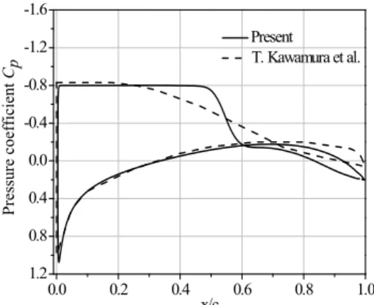
The comparisons of the pressure distribution on the foil surface for σ=0.8 is shown in Fig.3. It compares the present result with that of Kawamura and Sakuda (2003). There exists a good agreement but some difference in magnitude may be due to k-ω turbulence model used by Kawamura and Sakuda (2003).The
difference in pressure distribution on the face side is found very small. Similar comparison is shown in Fig.4 for σ=0.4. The time history of the lift and drag coefficients computed by mixture model at σ = 0.8 and σ = 0.4 are shown in Fig. 5. The characteristics of the curve of lift and drag coefficients are almost similar. The contours of pressure coefficient and vapor volume fraction for cavitation numbers σ=0.8 and 0.4 are shown in Fig.6. These contours show the expansion of cavity and their sizes for different cavitation numbers. At σ=0.8 the half of the hydrofoil is covered with vapor and at σ=0.4 the back surface is fully covered with vapor. It is clearly seen that the cavity length increases with the decrease in cavitation number.
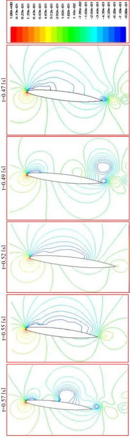
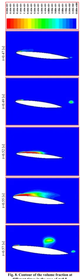
Figs.7 and 8show the instantaneous field of pressure distribution and vapor volume fraction respectively computed for five time levels t=0.47s, 0.49s, 0.52s, 0.55s and 0.57s in the case of σ=0.8. These figures clearly show the creation and collapsing of cavity over the hydrofoil surface.
Fig. 3. Comparison of the pressure coefficient on the foil surface at σ=0.8.
Fig. 4. Comparison of the pressure coefficient on the foil surface at σ=0.4.
0.0 0.2 0.4 0.6 0.8 1.0 1.2
0.8 0.4 0.0 -0.4 -0.8 -1.2 -1.6
Present T. Kawamuraet al.
Pressu
re coefficien
t
Cp
x/c
0.0 0.2 0.4 0.6 0.8 1.0
1.2 0.9 0.6 0.3 0.0 -0.3 -0.6
P
ress
u
re
co
ef
fi
cien
t
Cp
Fig. 5(a). Time history of lift coefficient at σ=0.8.
Fig. 5(b). Time history of drag coefficient at
σ=0.8.
Fig. 5(c). Time history of lift coefficient at σ=0.4.
Fig. 5(d). Time history of drag coefficient at
σ=0.4.
Fig. 6(a).Contour of pressure coefficient at
σ=0.8.
Fig. 6(b).Contour of pressure coefficient at
σ=0.4.
It is observed that the length of sheet cavity grows gradually until the cavity trailing edge almost reaches the end of a foil, and then reverse flow emerges near the foil trailing edge.
Fig. 6(c). Contour of vapor volume fraction at
σ=0.8.
0.0 0.1 0.2 0.3 0.4 0.5 0.6
-0.25 0.00 0.25 0.50 0.75 1.00 1.25
Lift Coefficie
n
t
CL
Time [s]
CL
0.0 0.1 0.2 0.3 0.4 0.5 0.6
-0.03 0.00 0.03 0.06 0.09 0.12 0.15 0.18
Drag
Co
o
eff
ic
ien
t
CD
Time [s]
CD
0.0 0.1 0.2 0.3 0.4 0.5 0.6
0.1 0.2 0.3 0.4 0.5 0.6
L
ift Coeffic
ient
C
L
Time [s]
CL
0.0 0.1 0.2 0.3 0.4 0.5 0.6
0.06 0.07 0.08 0.09 0.10 0.11 0.12
CD
D
ra
g
Cof
fic
ie
nt
CD
Fig. 6(d). Contour of vapor volume fraction at
σ=0.4.
The reverse flow propagates towards the leading edge along the back surface of edge foil causing collapse of the sheet cavity.
Table 5 shows the summary of the cavitation parameters where, , and are maximum cavity length, maximum cavity thickness and the position of cavity thickness respectively. As the cavitation number decreases, the maximum cavity length and maximum cavity thickness increase. On the other hand, the position of maximum cavity thickness is almost constant at 75% of the maximum cavity length except for σ = 0.4. In the case of σ = 0.4, a super cavitating flow fully develops and the cavitation also appears on the pressure side near the trailing edge. It is also seen that the time-averaged lift coefficient decreases and the time-averaged drag coefficient increases as the cavitation number decreases. However, after σ=0.9, it decreases slightly. Fig. 9 shows the variation of maximum cavity length and thickness with the cavitation numbers. The change pattern of unsteady cavitation is observed in this figure.
Table 5 Summery of different cavitations parameter
σ lmax tmax ltmax CL CD
3.5 - - - 0.667 0.024
1.5 0.098 0.0211 0.76 0.582 0.0378
1.2 0.16 0.0329 0.79 0.57 0.0425
1.1 0.21 0.0465 0.73 0.566 0.0446
1.0 0.25 0.047 0.73 0.560 0.0476
0.9 0.45 0.0772 0.78 0.51 0.0783
0.8 0.49 0.0784 0.71 0.44 0.077
0.4 1.00 0.28 0.66 0.214 0.0763
t=
0.
47
[s
]
t=
0
.49
[
s]
t=
0
.52
[
s]
t=
0
.55
[
s]
t=
0.
57
[s
]
t=0.47
[s
]
t=
0
.49
[
s]
t=0.52
[s
]
t=
0.55
[
s]
t=
0.57
[
s]
Fig. 8. Contour of the volume fraction at different times in the case of σ=0.8.
8. CAVITATING
FLOW
AT
DIFFERENT ANGLE OF ATTACK
In this section, the cavitating flow on the CAV2003 hydrofoil at different angles of attack is discussed for cavitation number σ = 0.8. Flow over the hydrofoil with a positive attack angle causes sharp pressure and velocity gradients near the nose.
Table 6 Predicted lift and drag at different angles of attack
Angle of attack
L
C CD
= ° 0.4085 0.021
= ° 0.425 0.0525
= 7° 0.44 0.077
Table 6 shows the predicted lift and drag
coefficients at angles of attack
4,
5and 7
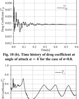
for cavitation number, σ=0.8. As the angle of attack increases both the lift and drag coefficients gradually increase. Fig.10 shows the time history of lift coefficient and drag coefficients at different angles of attack. These coefficients also oscillate around the time-averaged value.Fig. 9.Variation of maximum cavity length and maximum cavity thickness with cavitation
number.
Fig. 10 (a). Time history of lift coefficient at angle of attack = °for the case of σ=0.8.
0.2 0.4 0.6 0.8 1.0 1.2 1.4 1.6
0.0 0.3 0.6 0.9 1.2 1.5
0.0 0.1 0.2 0.3 0.4 0.5
Maximum cavity
th
ick
n
ess
Maximum cavity length
Ma
xi
mum
c
av
ity
le
ng
th
Cavitation number Maximum cavity thickness
0.0 0.1 0.2 0.3 0.4 0.5 0.6
0.36 0.39 0.42 0.45 0.48
Lift C
o
ef
ficie
n
t
CL
Time [s]
Fig. 10 (b). Time history of drag coefficient at angle of attack = °for the case of σ=0.8.
Fig. 10(c). Time history of lift coefficient at angle of attack = °for the case of σ=0.8.
Fig. 10 (d).Time history of the drag coefficient at the angle of attack = ° for the case of σ=0.8.
9. CONCLUSION
Two-dimensional finite volume method has been applied to simulate incompressible flow around CAV2003 hydrofoil. Three turbulence models are used to capture boundary layer in the simulation of steady flow around hydrofoil. It is observed that the RNGk-ε model with enhanced wall treatment and Spalart-Allmaras model compute the lift coefficient accurately. However, only RNGk-ε model with enhanced wall treatment is used for simulation of cavitating flow because of its better performance. For cavitation number σ=0.8, an unsteady partial cavitating behavior and for cavitation number σ=0.4, an unsteady super cavitating behavior are observed. The instantaneous pressure distribution
and vapor volume fraction computed are shown at different time steps. Therefore, it is clearly understood that the length of the sheet cavity grows gradually towards the trailing edge and reverse flow emerge near the foil trailing edge and propagates towards the leading edge and causing the creation and collapsing of cavity over the hydrofoil surface. Moreover, analysis is done for different cavitation numbers and the computed maximum cavity length and maximum cavity thickness show good correlation with cavitation numbers.
Finally, simulation of cavitating flow has been done at different angles of attack. Presence of hydrofoil with a positive angle of attack causes the sharp pressure and velocity gradient near the nose. The lift force and drag force increase with the increase in angles of attack.
ACKNOWLEDGEMENTS
The authors thankfully acknowledge BUET for providing research facilities and financial support for this research.
REFERENCES
Alajbegovic, A., H. A. Groger and H. Philipp (1999). Calculation of transient cavitation in nozzle using the two-fluid model.12thAnnual
Conference on Liquid Atomization and Spray Systems, Indianapolis, IN, USA.
Brennen, C. E. (1995). Cavitation and Bubble Dynamics.Oxford University press, Oxford. Coutier-Delgosha, O. and A. A. Jacques (2003).
Numerical reduction of cavitating flow on a two–dimensional symmetrical hydrofoil with a single fluid model. Fifth International Symposium on Cavitation(Cav2003), Osaka, Japan.
Delannoy, Y and J. L. Kueny (1990). Two phase flow approach in unsteady cavitation modelling, Cavitation and Multiphase Flow Forum, ASME-FED 98, 153–158.
Dular, M., R. Bacher, B. Stoffel and B. Širok (2005). Experimental evaluation of numerical simulation of cavitating flow around hydrofoil. European Journal of Mechanics B/Fluids 24, 522-538.
France, J. P. and J. M. Michel (2004). Fundamental of cavitation. Kluwer academic publishers.
Frobenius, M., R. Schilling, R. Bachert and B. Stoffel (2003). Three-dimensional unsteady cavitation effects on a single hydrofoil and in a radial pump – measurements and numerical simulations, Part two: Numerical simulation. Proceedings of the Fifth International Symposium on Cavitation, Osaka, Japan.
Karim, M. M., N. Mostafa and M. M. A. Sarker (2010). Numerical study of unsteady flow around a cavitating hydrofoil, Journal of Naval
0.0 0.1 0.2 0.3 0.4 0.5 0.6
0.012 0.015 0.018 0.021 0.024 0.027 0.030 0.033
D
rag C
o
eff
icie
n
t
CD
Time[s]
CD
0.0 0.1 0.2 0.3 0.4 0.5 0.6
0.0 0.2 0.4 0.6 0.8 1.0
Lif
t Coeffi
cient
CL
Time [s]
CL
0.0 0.1 0.2 0.3 0.4 0.5 0.6
0.00 0.02 0.04 0.06 0.08 0.10 0.12
CD
D
rag coefficie
n
t
CD
Architecture and Marine Engineering, 7(1), 51-61.
Kawamura and T. M. Sakuda (2003). Comparison of bubble and sheet cavitation models for simulation of cavitation flow over a hydrofoil. Fifth International Symposium on Cavitation(Cav2003), Osaka, Japan.
Kubota, A., A. Hiroharu and H. Yamaguchi (1992). A new modeling of cavitating flows, a numerical study of unsteady cavitation on a hydrofoil section. Journal of Fluid Mech. 240, 59–96.
Mostafa, N. (2009). Numerical simulation of cavitating flow over a hydrofoil using finite volume method, M.Phil. Thesis, Bangladesh University of Engineering and Technology, Bangladesh.
Pouffary, B. R. Fortes-Patela and J. L. Reboud (2003, November). Numerical simulation of cavitating flow around a 2D hydrofoil: A
barotropic approach. Fifth International Symposium on Cavitation(Cav2003), Osaka, Japan.
Schnerr, G. H. and J. Sauer (2001). Physical and numerical modeling of unsteady cavitation dynamics. 4thInternational Conference on
Multiphase Flow, ICMF-2001, New Orleans, USA.
Singhal, A. K., H. Li, M .M. Atahavale and Y. Jiang (2002). Mathematical basis and validation of the full cavitation model. Journal of Fluids Eng. 124, 617–624.
Stutz, B. and J. L. Reboud (2002). Measurements within unsteady cavitation. Exp. Fluids 29, 545-552.