Submitted19 November 2015 Accepted 6 July 2016 Published16 August 2016 Corresponding author Johannes M. Baveco, hans.baveco@wur.nl
Academic editor Mattias Jonsson
Additional Information and Declarations can be found on page 21
DOI10.7717/peerj.2293
Copyright 2016 Baveco et al.
Distributed under
Creative Commons CC-BY 4.0 OPEN ACCESS
An energetics-based honeybee
nectar-foraging model used to assess the
potential for landscape-level pesticide
exposure dilution
Johannes M. Baveco1, Andreas Focks1, Dick Belgers1, Jozef J.M. van der Steen2,
Jos J.T.I. Boesten1and Ivo Roessink1
1Alterra, Wageningen University and Research, Wageningen, The Netherlands
2Plant Research International, Wageningen University and Research, Wageningen, The Netherlands
ABSTRACT
resource patches (crop fields) both versions predicted the use of a small number of patches.
SubjectsAgricultural Science, Conservation Biology, Ecology, Entomology, Environmental Sciences
Keywords Honeybee, Foraging, Landscape ecology, Pesticide exposure, Energetic efficiency, Flower strips, Semi-natural habitats, Resource selection, Depletion, Nectar content
INTRODUCTION
There is serious concern about the widespread decline of pollinators in the agricultural landscape (Potts et al., 2010;Vanbergen et al., 2013). Agricultural intensification leading to increased stress from pesticides and lack of floral resources, is probably the main cause (Goulson et al., 2015). Honeybees, by exploiting mass-flowering crops, operating over long distances, and by being carefully managed by beekeepers, can be considered to be relatively insensitive to the disappearance and deterioration of semi-natural elements providing food and nesting opportunities (Ricketts et al., 2008;Sponsler & Johnson, 2015;Winfree et al.,
2009). Their dependence on cropland for nectar and pollen acquisition, however, leads to
high potential exposure to pesticides (Krupke et al., 2012).
Understanding to what extent pesticides may affect honeybees requires as an essential first step the quantification of their potential exposure. Exposure at the hive is the outcome of foraging in the landscape surrounding the hive, as concentrations of pesticides in nectar and pollen brought by foraging bees will depend on the provenance of these food items, and thus on choice of forage and foraging locations (Garbuzov et al., 2015). It is well known that honeybees may forage over long distances (Beekman & Ratnieks, 2000), up to approximately 10 km away from the hive. However, when sufficient high-quality resources are available nearby, most foraging will take place within a few kilometres (Couvillon et al., 2015;Couvillon, Schurch & Ratnieks, 2014b).
Models considering foraging in complex, heterogeneous landscapes with multiple resources to choose between, can be used to predict exposure concentrations at the bee hive. Such models may also serve as tools to test landscape management measures aimed at lowering exposure risk (mitigation). However, of the numerous honeybee models reviewed inBecher et al. (2013)andSchmickl & Crailsheim (2007), none were developed to address landscape-level foraging and its consequences for pesticide exposure.
We extend and adapt the energetics-based modelling approach (Cresswell, Osborne
which conditions the presence of multiple resources can divert foraging effort away from pesticide-treated fields and lead to dilution of exposure: a possible explanation of lower observed ‘‘field-realistic’’ rates of exposure compared to laboratory studies (Carreck & Ratnieksi, 2014).
We finally explore whether landscape management aimed at pollinator conservation may have the additional benefit of lowering the exposure of honeybees to pesticides. Three hypothetical scenarios were tested for their impact on exposure dilution, through the presence of attractive alternative crop fields, flowers strips (off-crop in-field resources), or attractive resources on off-field habitats.
MATERIAL & METHODS
Energetics-based foraging model
The model simulates honeybee nectar foraging over a single day in hourly time steps. The model ignores in-hive colony dynamics and assumes the colony to have limited to perfect knowledge of available resources and to adapt quickly to environmental fluctuations in food conditions (Beekman & Lew, 2008;Beekman, Oldroyd & Myerscough, 2003). Resource patch selection is based on net energetic efficiency. We differentiate between two basic model versions. In the ‘‘single-optimal’’ (SO) version of the model we assume that the colony’s self-organization is fast enough to effectively focus on the single most-profitable food patch each hour. In case of two or more approximately equally profitable sources, mechanisms should be present that reinforce the use of only one of them (e.g., symmetry breaking and cross inhibition (De Vries & Biesmeijer, 2002)). In the ‘‘recruitment-limited’’ (RL) version we acknowledge that the rate of recruitment of foragers for a resource limits the speed with which the system can adjust to dynamic resources (Seeley & Visscher, 1988). As a consequence, in this version several resource patches with a high net energetic efficiency can be exploited simultaneously, as suggested by field observations (Beekman et al., 2004;
Visscher & Seeley, 1982). In the SO-model this may occur when resource availability changes during the day, depending on the anthesis of flowers and/or due to resource depletion. In the RL-model, simultaneous exploitation of multiple patches during the day is the rule.
The model predicts for a hive at a specific location the set of resource patches used during a single day as well as several quantities that can be compared to field observations, e.g., the amount of sugar arriving at the hive, exploited nectar sources weighted by the amount of collected sugar in each, or the distribution of foraging distances. Alternatively, it allows for the quantification of impact of the hive population on a crop, e.g., as the number of flower visits per unit area, per flower or per patch.
Landscape and resources
Foraging takes place in a landscape consisting of multiple resource patches. Each resource patch is assumed to be internally homogeneous and to contain a single resource. Resource patches may be fields with mass-flowering crops providing nectar or semi-natural habitats characterised by a dominant nectar-providing species.
Resources have a dynamic density of nectar-providing flowersF (m−2). In absence of
density and the number of open flowers per plant. Resources are characterised by the
average amount of nectarg (mg) a honeybee can obtain from a flower, and by the typical
sugar content of its nectar (g g−1).
Resource patch selection
Being a central-place forager, a honeybee foraging trip comprises the travel back and forth between hive and resource patch, and the searching for and handling of flowers in the patch. Within the field, floral resources are collected assuming a type II functional response (Holling, 1959), so the number of flowers with nectar that are visited per time unit (s) amounts to
f = aF
1+ahF (1)
withathe attack rate (m2s−1) andhthe handling time per flower (s). The rate of nectar
collection (mg s-1) is given byfg. The timetLit takes to collect nectar to full capacity is
tL=
γ
fg (2)
where the capacity is given byγ (mg). Note that unlike e.g.,Schmid-Hempel, Kacelnik & Houston (1985)we assume that foragers always collect a full load.
Flight time and flight costs are proportional to the distance from hive to the resource patch. The duration of a foraging trip equals the sum of travel times and the time spent at the patch:
ttrip=2 D v +
γ
fg (3)
withDbeing the distance from the hive to the field (m), andvthe flight velocity (m s−1).
The energy expenditure EE (J) ignoring basic metabolism can be calculated as the
sum of the travel costsEEtravel(travel time×energetic costs per time unit) and the costs
while loading nectar in the fieldEEfield. The latter term is made up by flight costs while
searching for nectar flowers and costs while sitting on the flowers extracting the nectar. The latter is ignored, as it is approximately an order of magnitude smaller than flight costs (a value of 0.0042 J s−1was applied inSchmid-Hempel, Kacelnik & Houston (1985)). Energy expenditure at the field thus becomes:
EEfield=
tL−
γ
gh
eF=
γeF
gaF. (4)
The equation is simplified by substitutingEqs. (2)and(1), thus eliminating the handling
time. By assuming that handling the flower doesn’t take energy,hdoes not play a role in
the energetic balance. InEq. (4)average flight costeF (J s-1) is used, as during foraging in
the field the individual state changes gradually from unloaded to loaded. The value ofeF
is obtained from loadedeF,L and unloadedeF,U flight costs (Seeley, 1986). The total travel
costs are given by:
EEtravel= D
v eF,U+eF,L
=2D
If the same route is followed back and forth, the energy costs can be averaged. The total energy expenditureEEtotal(J) for a foraging bout sums to:
EEtotal=
tL−
γ
gh
eF+2
D veF=
tL−
γ
gh+2 D v
eF=
γ
gaF+2 D
v
eF. (6)
The yield of a trip in terms of energy, energy intakeEI(J), depends on the energy content of the collected nectar of resource typeR,eR(J mg−1):
EI=γeR. (7)
Withttrip,EEandEI, the basic ingredients for a ‘‘decision-making process’’ for a colony are
specified, and costs (both in energy and time) and yields for specific foraging locations in a landscape with multiple fields can be compared. In theory, there are different currencies that might be optimized (Stephens & Krebs, 1987). For honeybees, considerable effort has been invested in deciding whether the relevant currency is the net rate of energy delivery ((gain−cost)/time) or the net energetic efficiency ((gain−cost)/cost). Experimental data,
e.g., Seeley (1994)but seeDe Vries & Biesmeijer (2002), and models fit to experimental data (Schmid-Hempel, Kacelnik & Houston, 1985), as well as several of the other foraging models discussed byBecher et al. (2013)indicate that net efficiency is the most appropriate
currency. We therefore assume that net energetic efficiencyNEE
NEE=EI−EEtotal EEtotal
(8)
defines the attractiveness of each patch. In the SO version, the patch with maximumNEE
is selected as the single resource patch. In the RL version, the recruitment of foragers for a resource patch is explicitly modelled, following Camazine & Sneyd (1991)andSeeley, Camazine & Sneyd (1991)and extending their model in a somewhat similar way as done byCox & Myerscough (2003). In the RL-model,NEE is translated into the probability of foragers abandoning resources and recruiting new foragers among the follower-bees present at the dance floor (Supplemental Information 2).
Resource detection
Resource patches are detected primarily by scouts. Scouts make up around 10% of the unemployed foragers: novice foragers and experienced foragers that have recently
abandoned a depleted resource patch (Seeley, 1995). Detection of an attractive resource
patch may depend on patch distance and size (Dauber et al., 2010), as well as on the
number of active scouts. Encounter rates may be obtained from movement models or from dispersal functions summarizing movement simulations (Heinz et al., 2007) asσi values:
the probability that a single scout encounters patch i. The probability for patchi being detected by at least 1 ofsscouts amounts to
Pi=1−(1−σi)s. (9)
dealing with a landscape with abundant resources in the immediate surroundings of the hive (Seeley, 1995).
Resource acquisition
The colony’s hourly acquisition of a selected resource depends on the absolute number
of foragersndedicated to this resource. For the SO-model,nequals the total number of
foragers active in a time step. For the RL-model, nis a fraction of this total number, as multiple patches may be exploited simultaneously. Foragers may make several trips to
the same patch, depending on trip durationttripand the time between trips tUDspent
on unloading and dancing in the hive. Thus, the number of foraging trips per hour an individual forager can make, amounts to b=1t/(ttrip+tUD) with1t representing the
time step in seconds.
Not the full load of nectarγ collected in the patch will arrive at the hive as some of the sugar will be consumed on the way back. The amount of energy used during the return flight,Ec, is approximatelyeLDv. The amount of nectar arriving at the hive thus decreases
toγ−Ec
eR per trip and when summed over all foragers exploiting the patch during this time step becomes:
n
γ−Ec eR
b. (10)
Resource dynamics
By calculating resource patch selection per hour we may account for: (1) any diurnal pattern in the anthesis of flowers; (2) depletion of floral resources occurring in small resource patches; and (3) diurnal patterns in the number of active foragers in the hive. For simplicity’s sake, we assume a binary pattern in anthesis (all flowers either open or closed). Resource dynamics may also result from nectar consumption by competing species or
foragers from other colonies. A constant background density of competitors,Z, may be
defined of species that exploit resources in a similar way as honeybees (same functional response). The main reason to incorporate competition is that it allows us to explore honeybee foraging in a setting of quickly depleting resources.
Within a day there may be also renewal of nectar resources. With a non-zero renewal rate, r, a fraction of the pool of visited (empty) flowers will each time step turn into nectar-providing flowers again.
We deal with resource depletion by subtracting after each time step the visited number of open flowers from the initially present number. Hourly dynamics in open flower density
F are given by:
Ft+1=Ft−
nγ
gAb− aFt
1+ahFtZ+r(F0−Ft) (11)
withArepresenting field size (m2). A fixed number of flowersγ /g is visited for a full load.
Lowered flower density may change theNEE-based ranking of resource patches in the next
Exposure Assessment
When the foraging model is combined with information on fields being treated with a chemical, and/or off-field habitats being exposed to spray-drift, the concentration of the chemical in the nectar brought into the hive can be estimated. It depends on the concentration of the chemical in the nectar of flowers in exploited patchi,Ci, expressed in
e.g.,µg mg−1. When the chemical is not metabolized together with the sugar on the way back to the hive, its total amount (mg) arriving at the hive will be:
L
X
i=1
niγbiCi. (12)
The summation is made overL, the set of all exploited patches over all hours. The
concentration of the chemical in nectar at arrival no longer equals Ci but becomes
Ci/
1− Ec,i γeR,i
, implying enrichment. When the chemical is metabolized together with the sugar, its concentration in the nectar remains the same but the amount arriving at the hive will be lower:
L
X
i=1 ni
γ−Ec,i eR,i
biCi. (13)
From the point of view of exposure risk inside the hive, the relevant chemical concentration should be expressed on a sugar base: nectar with a low sugar content will be concentrated until a minimum sugar content is reached. The exposure on a sugar-base is obtained by
dividing the total amount of the chemical (µg) entering the hive by the total amount of
sugar entering the hive (mg). Without metabolization of the chemical (with enrichment) we obtain as sugar-based daily-averaged concentration of the chemical (µg mg-1) entering the hive:
Xe=
PL
i=1niγbiCi
PL
i=1ni(γeR,i
−Ec,i)
eSUGAR bi
. (14)
When the chemical is metabolized with the sugar (no enrichment) we obtain:
Xm=
PL
i=1ni(γ−EeRc,,ii)biCi
PL
i=1ni(γeR,i
−Ec,i)
eSUGAR bi
. (15)
Equations (14)and(15)quantify the contribution of each selected resource patch to the sugar-based concentration of a chemical (µg chemical mg-1sugar) entering the hive. Using this information together with the calculated amount of sugar having this concentration we can construct detailed distributions quantifying the relative composition of the nectar entering a particular hive, in terms of sugar-based concentrations.
Dilution
to a reference concentration in treated resources, e.g., the sugar-based concentrationXPin
the nectar of a treated field with resourceR:
XP=CP
eSUGAR eR
(16)
whereCP refers to the concentration (on a wet-weight base) in nectar on the treated
field, often referred to as the predicted environmental concentration (PEC) resulting from a certain application rate of the chemical. It is multiplied byeSUGAR/eR to obtain the
sugar-based concentration. Dilution factors follow from actualXm orXe as:
ϕm=Xm/XP andϕe=Xe/XP. (17)
With a patch-specific Cwe can represent variability in the applied dose for the treated
crop, deal with a substance that is applied on different crops with different doses, and include patches representing off-crop or off-field habitats that are exposed through spray drift only.
For an agricultural landscape containing fields with a target crop as the only resources,
Eqs. (14)and(15)can be further simplified. With a single resourceeR,iequalseRand when
application of a pesticide on the target crop leads to a constant concentrationCPin the
nectar,CiequalsCP. Dilution obtained applyingEq. (14)then simplifies to:
ϕe=
PL
i=1niγbiCP
PL
i=1ni(γeR
−Ec,i)
eSUGAR bi
1
CPeSUGAReR
=
PL
i=1δiniγbi
PL
i=1ni(γeR−Ec,i)bi
(18)
withδi=1 in case the field selected in time stepiis sprayed andδi=0 if it is unsprayed.
Similarly, for the case with metabolization and no enrichment (Eq. (15)) we obtain:
ϕm=
PL
i=1δini(γ−EecR,i)biCP
PL
i=1ni(γeR
−Ec,i)
eSUGAR bi
1
CPeSUGAReR
=
PL
i=1δini(γeR−Ec,i)bi
PL
i=1ni(γeR−Ec,i)bi
. (19)
Eqs. (18)and(19)show that for this simplified case, dilution factors do not depend on
CP but simply reflect how many unsprayed fields are selected. When all selected fields are
treatedϕmwill be one, whileϕemay even exceed one. Whether selected resource patches
were treated or not depends on the application scenarios. In a probabilistic approach, with prepresenting the probability for a field of being treated, dilution will on average approximatep.
90thpercentiles
Model Analysis & Application
Energetics-based model
From the energetics-based model (Eqs. (6) and(7)) we derived thresholds for the
exploitation of resources depending on distance and resource characteristics, as done by
Cresswell, Osborne & Goulson (2000). For resources at equal distance we derived a simple equation to compare their attractiveness. For landscapes consisting of only large-scale crop fields, we derived rules of thumb for the selection of foraging locations.
Landscape representation
When it is assumed that nectar is collected from all resources in the landscape proportional to their attractiveness (EFSA, 2013), exposure dilution is always to be expected in landscape mosaics with multiple resource patches. In the RL-model dilution is more likely than in the SO-model. To explore whether landscape-level exposure mitigation can be effective, we tested for both models three scenarios, all based on the idea that by providing alternative floral patches foraging effort can be diverted away from exposed patches. Construction of flower strips and pollinator-friendly management of semi-natural habitats are such measurements that may contribute to the persistence of pollinator populations in the agricultural landscape (Garibaldi et al., 2014;Haaland, Naisbit & Bersier, 2011;Wratten et al., 2012). Also, the presence of different (early and late) mass-flowering crops has been suggested to enhance pollinator density (Riedinger et al., 2014).
We parameterized the model for two flower species (Table 2), oilseed rape (Brassica napus, OSR) as a common attractive mass-flowering crop, and white clover (Trifolium repens) being an important floral resource, common along roadsides and field margins (Sponsler & Johnson, 2015). Patches with these resources provided the building blocks of the landscapes tested in the scenarios. In all scenarios OSR represented the target crop. From the model it followed that for any of the scenarios to be effective the alternative
resource had to be equally or more attractive (larger NEE at equal distance) than the
OSR field. For the scenario study, using a hypothetical landscape, we selected for OSR a conservative and for clover an optimistic estimate of the relevant coefficients (Table 2and
Supplemental Information) and checked whether this condition was met (see ‘Results’). In real landscapes clearly more resource types will be present, in a range of densities. To understand the impact of some of this variability we varied flower densities and sugar content over a range of values.
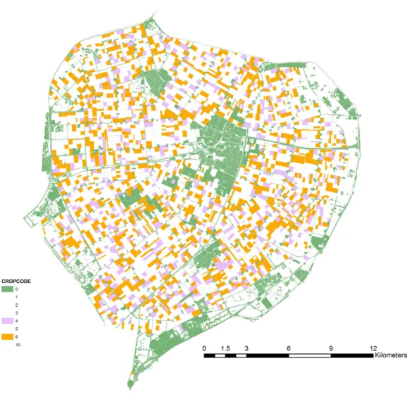
We defined landscape structure from geographic data for the northern part of Flevoland (The Netherlands). Geo-referenced data for crops were obtained from the land-use database LGN6 (grid-based, 25 m resolution) (Hazeu et al., 2011). Data on the presence of off-field habitats (road side verges, ditch sides, shores, other semi-natural elements) were obtained
from the vector-based dataset TOP10NL (PDOK, 2015). We assumed that fields of LGN6
category ‘‘other crops’’ represented OSR. For the ‘‘Alternative Fields’’ scenario, fields of another (randomly chosen) LGN6 category represented the alternative mass-flowering crop (Fig. 1). For the ‘‘Off-field Habitats’’ scenario, off-field habitats were used as specified in the spatial data set. All sites (cells in the 25 m grid) that bordered target crop fields were
Figure 1 Map of the case-study area.Oilseed rape fields (ochre), alternative crop fields (lilac) and off-field resource patches (green) as used in the scenario simulations.
the model was finally run on a random selection of 10% of these sites (identical for all scenarios and runs). Tested landscapes contained 1,207 fields with OSR (7,057 ha). The alternative crop was present on 454 fields (3,375 ha). Off-field habitat patches were small and numerous: 58,137 patches comprising 3,410 ha.
We assumed all resources to have open flowers during the whole day, a foraging day of 10 h, no competitors being present (Z=0), no renewal of resources (r=0), 100 active
foragers and coefficients as in Tables 1and2. By definition, sites were next to a large
resource patch. Therefore, considering only resources within 2 km distance (Dmax=2000)
and assuming perfect knowledge of their presence (P=1 for each resource patch) seemed
Table 1 Fixed (energetic) coefficients for honeybee and nectar.
Coefficient Symbol Dimension Value Source
Maximum foraging distance
Dmax m 2000a
Flying speed v m s−1 4.17b de Vries & Biesmeijer
(1998)
Flight cost (unloaded)
eU J s-1 0.037c Seeley (1986)
Flight cost (loaded) eL J s-1 0.075 Seeley (1986)
Capacity (maximum load)
γ mg 32.5 Winston (1987)
Energetic value sugar eSUGAR J mg-1 17.2 Seeley (1985)
Time unloading nectar and dancing
tUD s 300d Seeley, Camazine &
Sneyd (1991)
Notes.
aSpecific for studied scenarios. Considerably longer distances have been reported, e.g. max. 13.5 km, 95% within 6 km, mean
2.3 km (Beekman & Ratnieks, 2000).
bOther reported value 6.95 m s-1(Seeley, 1995).
cOther reported value 0.0334 J s-1(Schmid-Hempel, Kacelnik & Houston, 1985and references therein).
dGoodwin et al. (2011)observed longer times in the hive between foraging (11.13 min). Range 150–300 in the model ofSeeley, Camazine & Sneyd (1991).
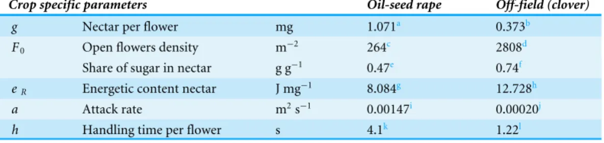
Table 2 Resource-specific coefficients.Coefficient values for the two resources considered in the study, oilseed rape and clover.
Crop specific parameters Oil-seed rape Off-field (clover)
g Nectar per flower mg 1.071a 0.373b
F0 Open flowers density m−2 264c 2808d
Share of sugar in nectar g g−1 0.47e 0.74f
eR Energetic content nectar J mg−1 8.084g 12.728h
a Attack rate m2s−1 0.00147i 0.00020j
h Handling time per flower s 4.1k 1.22l
Notes. aRange 0.7–6
µl (average 2.0µl) (Pierre et al., 1999), approximately 0.7+0.7∗0.53=1.071to 6+6∗0.53=9.18 mg.
bRange 0.143–0.351 (10◦C) and 0.112–0.373 (18◦C) (Jakobsen & Kritjánsson, 1994).
cOwn measurements: (June 2014: 1182; September 2015: 264).
dGoodwin et al. (2011)for clover field, defined as density of open florets (=15.6 open florets per flower x 180 flowers m−2). Burdon (1983): 1500–3000 open flowers, derived from 20–40 florets per head (average 30), assuming 50 –100 flower-heads per m2.
eRange 0.47–0.59 compiled fromPritsch (2007)andMaurizio & Grafl (1969). fJakobsen & Kritjánsson (1994).
g,hFrom (share of sugar) *e SUGAR. i,jSeeSupplemental Information 1.
kFree & Nuttall (1968).
lPeat, Tucker & Goulson (2005)for small bumblebee.
Exposure mitigation
(i) Alternative Fields: dilution can result from the presence of attractive but untreated fields, either with the target crop or with alternative attractive (mass-flowering) crops. For crop fields other than the one nearest to the hive, treatment occurred following a probability
realizations of the series of treated fields. The analysis was done for a range of values forp
(0–1, with an interval of 0.1). A variant of this mechanism would be the presence of fields with another, attractive, crop type. We tested this by defining another common crop in Flevoland as a hypothetical alternative mass-flowering crop, largely identical to oilseed rape (Fig. 1). The energetic attractiveness of this crop was manipulated to range from less to more attractive than OSR, by adjusting its sugar content (0.8, 0.9, 1, 1.1 and 1.2 times OSR sugar content). Thus, the alternative crop could also represent another OSR variety. (ii)Flower Strips: dilution can result from the presence of highly attractive flower strips around target crop fields. This was simulated by adding to each target crop field up to 4 flower strips at its edges, each strip of length 1/4 of field perimeter. Strips contained white clover (Trifolium repens,Table 2) in densities comparable to clover fields. Presence of each strip was randomly set, with a probabilityp(0–1, with an interval of 0.1). The area of a flower strip was set to a prescribed widthwmultiplied by strip length. Width values of 1, 2, 5 and 10 m were tested. The area contained in the strips was subtracted from the crop field area. Thus, strips were strictly in-field off-crop habitats.
(iii)Off-field Habitats: dilution can result from the presence of off-field semi-natural habitats when these are managed in an appropriate way. We tested this using geo-data for
fields (as above) with OSR and for semi-natural elements (Fig. 1). We assumed a single
common flower species (white clover) to be representative for all off-field habitats. As the presence and size of these habitats were fixed and defined by the geo-data, we tested their impact on dilution for a range of resource quality values. Open flower density determined quality and was set to low, medium or high value (0.5, 1 or 1.5 times clover field density). The three quality levels were tested for a range of values for p, here representing the probability that an off-field element was considered a nectar resource patch.
RESULTS
Energetics-based model
From the energetics-based model (Eqs. (6) and(7)) we derived thresholds for the
exploitation of resources depending on distance to the resource patch and other resource characteristics. The energy balance (EI –EE) for a foraging trip has to be positive (Dukas & Edelstein-Keshet, 1998), leading to the condition:
γeR−
γ
gaF+2 D
v
eF>0. (20)
The threshold distance at which a resource patch cannot be exploited any more (Fig. S2) amounts to
DT=
vγ 2
eR
eF
−1 g
1
f −h
=vγ
2
eR
eF
− 1 gaF
. (21)
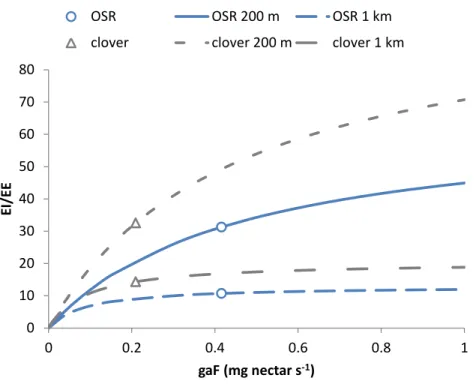
Resource patch selection based on net energetic efficiency implies selecting the
Figure 2 Choice of resources depends on net energetic efficiency.The choice between resources at equal distance depends on their value forEI/EE(Eq. (22b)). This ratio increases asymptotically with nectar ac-quisition rate gaFto the limit value 1/c×eR/eF. With largereR, e.g., for clover compared to OSR, EI/EE
will level off at a higher value. When flower density is much higher, the resulting value of EI/EEmay still be larger for the resource with the lowereR. Curves refer to resources at 200 m and 1 km. Values for clover
and OSR as specified inTable 2and used in the scenarios are indicated.
EI EE =
γeR
γ
gaF+2 D v
eF
(22)
This can be rewritten to:
EI EE =
gaF
1+2D
γvgaF
eR/eF. (22a)
Or, substituting 2γDv by constantcfor patches at equal distance:
EI EE =
gaF
1+cgaFeR/eF. (22b)
Figure 2 shows how this ratio depends on resource characteristicsgaF, the nectar acquisition rate. At equal distance, EI/EE scales linearly with energetic content eR and
asymptotically withgaF. In a mass-flowering case, a further increase of gaF will not
increaseEI/EEmuch. For a ‘‘sparse-flowering’’ resource to compete in attractiveness with a mass-flowering crop, its energy content or flower density needs to be considerably higher. An ‘extreme’ case results from landscapes consisting entirely of fields with mass-flowering
crops. There, open flower densityF will be very large, and the functional responsef will
zero andEEwill thus be determined mostly byEEtravel. The threshold distance (Eq. (21))
will simplify to a linear relationship witheR, with steepness independent of other crop
properties; the honeybee constants are given between brackets:
DT≈
γv
2eF
eR. (23)
Maximising the net energetic efficiency in the mass-flowering case means maximising
EI EE ≈
γv
2eF
eR
D. (24)
For fields at equal distance, the selected field will thus be the one with the highest energy contenteR.
Landscape scenarios
Cumulative distributions of dilution factors were discontinuous for the SO-model, with many sites experiencing no dilution at all, others having no exposure and some experiencing limited dilution (Figs. S3–S6). For the RL-model the distributions were continuous, with few sites being without exposure or without dilution. All distributions were summarized by their 10-, 50- and 90-percentiles (Fig. S6). For all scenarios the number of resource patches exploited over the day were obtained as well, as a characteristic output of the foraging model. For the RL-model, this referred to the number of resource patches accounting for 90% of the sugar brought to the hive.
“Alternative Fields”
In this scenario the number of resource patches and resource area were constant. In two sub-scenarios either only OSR fields or OSR fields plus fields with a similar crop of different quality (sugar content) were present.
When fields with OSR were the only resource patches, a smaller (SO-model) or larger (RL-model) fraction of the sites showed considerable dilution when a fraction of these fields were not sprayed (Fig. S3). Even when none of the fields besides the nearest were treated there was no site completely without exposure, indicating that the nearest (by definition treated) field was always included in the set of resource patches exploited during the day. For the RL-model, there was always some dilution, especially when the fields selected besides the nearest field had a high probability ofnot being sprayed.
In the presence of an alternative untreated crop there was a fraction of sites for which an alternative crop field was included in the set of exploited patches, resulting in dilution (Fig. S4). For the SO-model, these sites had no exposure at all, implying that this alternative crop field constituted the single patch exploited during the day. Depletion played no role on large fields and either the nearest OSR field or an alternative crop field was selected and remained optimal during the whole day. For the RL-model, there was always some dilution, but there were no sites completely without exposure as the nearby OSR field was always part of the exploited patches set.
The number of exploited patches over the day was on average small: one for the
chosen at the beginning of the day usually stayed the optimal one (SO-model) during the day, as depletion was unlikely on (large) fields. In this structurally simple landscape there were always only a few nearby attractive fields that were exploited simultaneously in the RL-model. With increased sugar content the distance over which the alternative crop was energetically attractive increased and thus the number of exploited patches became larger (RL-model).
“Flower Strips”
In this scenario the number of resource patches increased withp, the probability of a flower strip being present at a side of a OSR field. Total resource area remained constant, but the
ratio between the two resource types changed withw, strip width, as strips were located
in-field.
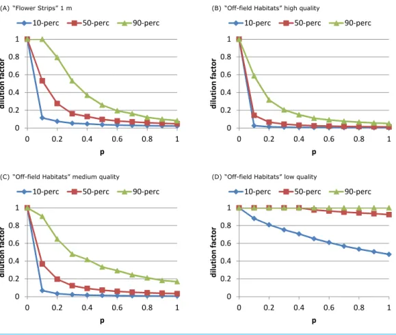
For both models the fraction of sites with considerable dilution increased profoundly withp(Fig. 3AandFig. S5). For the SO-model (Figs. S5andS6) increasing the width of strips increased the dilution reached by 90% of the sites. Wider strips could keep up a
higherNEE than the OSR field over a longer time, as depletion in the wider strips was
less likely. For the RL-model, impact of width was negligible: depletion was unlikely as foraging effort was already divided over multiple patches representing a relatively large area (including the OSR field).
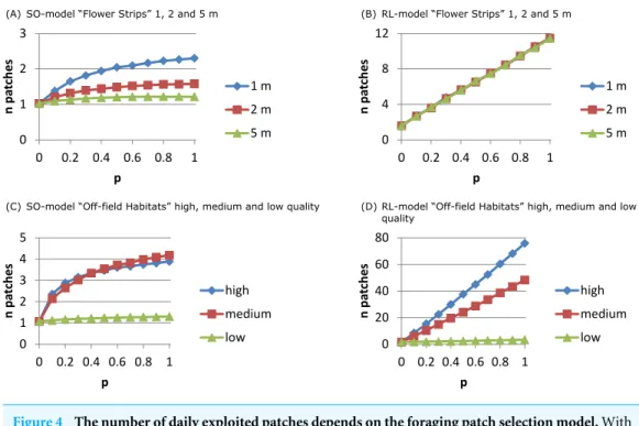
For the RL-model the number of exploited patches (Fig. 4B) increased linearly withp: more strips being present in the neighbourhood implied more patches being used. For
the SO-model (Fig. 4A) only with narrow strips the number of exploited patches per day
increased withp. Narrow strips were quickly depleted and when more strips were present
in the neighbourhood another strip could become the optimal patch of the next hour. Wider strips implied less depletion and strips being selected as optimal at the beginning of the day had a higher chance of remaining the single optimal patch during the day.
“Off-field Habitats”
In this scenario the number of resource patches and resource area increased withp, the
probability of an off-field habitat patch being managed for nectar resources of different quality (clover open flower density).
Presence of high quality off-field resource patches affected the distributions of dilution factors in a similar way as narrow flower strips (Figs.3B–3D,Fig. S6). The dilution factor cumulative distribution was very sensitive to off-field resource quality. With medium quality less dilution was reached at all sites and for low quality hardly any off-field resource patches were selected at all.
The number of exploited patches showed a similar pattern as in the flower strips scenario (Figs. 4Cand4D). For the SO-model with high and medium quality off-field habitats, the exploited patch number increased withpto 4 while for low quality it remained constant (1).
For the RL-model, exploited patch number increased linearly withpreaching a very high
Figure 3 Attractive flower strips and off-field habitats may dilute exposure.Flower strips can lead to high exposure reduction, when present in large numbers (A). For the RL-model, the width of the strips has no impact on this dilution; for 2, 5 and 10 m wide strips, the graphs are very similar (not shown). Off-field habitats can have similar impact (B, C) as flower strips. When quality is low (D) few off-Off-field habitat patches are selected resulting in little dilution. Note that flowers strips are identical to medium quality off-field habitat patches. All graphs refer to RL-model.
Comparing scenarios
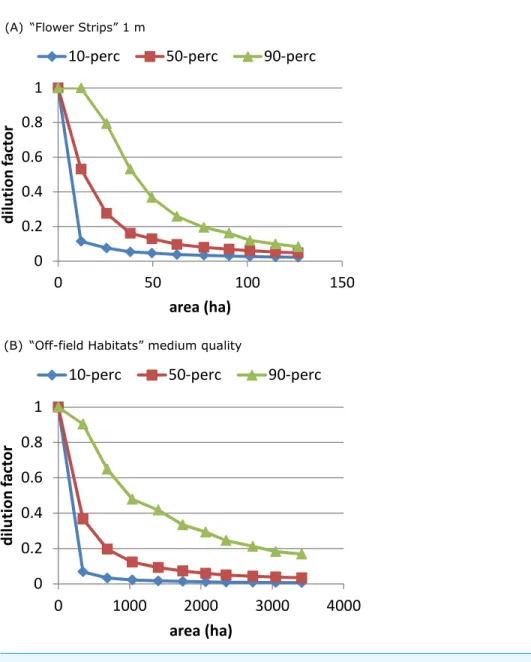
The ‘‘Flower Strips’’ scenario and ‘‘Off-field Habitats’’ medium quality scenario were similar as both created the same type of new resource patches, in-field versus off-field. We compared their effectivity by plotting the dilution percentiles against the total area covered by the patches. The ‘‘Flower Strips’’ scenario with narrow strips (1 m) appeared roughly 35 times as efficient as the ‘‘Off-field habitat’’ scenario (Fig. 5) as flower strips were in-field resource patches located always near the considered bee hive. Off-field resource patches on the other hand were not guaranteed to be sufficiently close to a target crop field and the bee hive site to have an impact.
DISCUSSION & CONCLUSIONS
Conceptual model
Figure 4 The number of daily exploited patches depends on the foraging patch selection model.With the SO-model an increase in the number of exploited patches indicates that depletion of the optimal patch plays a role. This may occur for narrow flower strips (A) and for off-field habitats that are mostly small-sized (C), and is determined by patch size not by its ‘quality’. For the RL-model the number of exploited patches is linearly related to their abundance. Depletion is unlikely and patch size has no impact on patch selection (B). Instead patch ‘quality’ is important (D) as patches need to have a sufficiently highNEEto be considered and promoted for in the recruitment process.
be made, and thus the colony’s rate of resource acquisition and of resource depletion. In a similar way, the size of a resource patch had no direct effect on its attractiveness, only indirectly through faster depletion of smaller patches. A smaller patch may also have
a larger probability of remaining undetected (Dauber et al., 2010). With a fixed number
of foragers exploiting a single patch (SO-model) or being distributed over a small set of patches (RL-model) the model predicted a decreasing flower visiting rate with patch size.
This seems in accordance with findings ofGoulson (2000).
The maximum distance at which nectar-providing resource patches can be exploited is given byEq. (21). Based on the values ofTables 1and2the distances estimated for OSR and clover fields, 8.1 and 12.7 km, respectively, are well within the range of maximum observed foraging distances. For these mass-flowering crops, the threshold distance is mainly defined by the energy content of their nectar (Eq. (23)). For natural elements with sparser flower distributions than found on clover fields, maximum distances are likely lower (Fig. 2), as searching times will be higher, increasing the energetic costs of traveling between flowers.
Resource patch selection
On a landscape level, the choice between resource patches depended on the relative value of their energetic efficiency. The attractiveness of different resources at different distances can
be compared with each other usingEq. (22), hence exposure mitigation strategies based
Figure 5 On an area-base flower strips are more effective than off-field patches.To obtain the same de-gree of dilution, much more area is required of managed off-field habitat patches (B), compared to flower strips (A) with identical properties. This is related to landscape characteristics and a consequence of off-field patches being in general further away from target crop off-field and hive location.
on our model. These alternative patches need to provide resources that are at least equally (RL-model) or more (SO-model) attractive.
patches accounting for in total 90% of the daily nectar collection. Assuming competition with other nectar-foraging species or other colonies (Fig. S11compared toFig. S8) indeed increased the number of exploited patches for the SO-model because of earlier depletion of the selected patch, while it decreased for the RL-model presumably because the total set of attractive patches over the day became smaller.
For a colony of feral honeybees in temperate deciduous forest, on average 9.7 (±4.9)
resource patches (pollen and nectar) accounted for 90% of the daily foraging activity (Visscher & Seeley, 1982). For two colonies of African honeybees in the Okavango River Delta,Schneider (1989)found that 16.2 (±9.6) and 17.5 (±5.9) sites/day accounted for
90% of the daily foraging activity on pollen and nectar. In both studies a continuous day-to-day redistribution of foragers over patches was observed, with many more patches
being present than used each day. Beekman and colleagues(2004)found for two large and
two small colonies of honeybees in an urban environment on average 15.8 and 15.0 patches being used per day (nectar and pollen), respectively.
These observations indicate that less optimization might happen than assumed in the SO-model, but also that less dilution of foraging effort is occurring than predicted by the RL-model for landscapes with many resource patches.
Landscape level exposure dilution
In current agro-ecosystems few high quality off-field resource patches will be available to honeybees (De la Rúa et al., 2009). The energetic model predicts that mass-flowering crops will be selected even when these are located at a large distance from the hive. Observations indeed indicate that in the period during which mass-flowering crops are available, these crops constitute the predominant nectar source (Requier et al., 2015). The off-field resource patches that are present will under these conditions experience pollinator dilution (Holzschuh et al., 2011), i.e., reduced wild plant pollination because OSR fields are preferred. Depletion is not likely to play a large role in these crop-dominated systems, as most crop fields are large and flower densities are in the saturating range of the functional response. The model thus suggests that in general there will be little potential for dilution of exposure in such landscapes, because the only resource that can be as attractive as a mass-flowering crop is another potentially sprayed mass-flowering crop.
were located within the target crop field, so they easily met the small distance condition. On the other hand, such a location in a target crop field may pose an additional exposure risk when crop treatment also causes exposure in the strips. With spray drift, effectiveness in attracting foragers may trade off against higher exposure risk for flower strips, and it might be possible to achieve a higher dilution for off-field patches that are carefully chosen with respect to their location relative to crop fields: close enough to attract foragers, but far enough to avoid contamination.
Model complexity and limitations of the predictions
The current application of the developed model was not meant to deliver accurate predictions of absolute real-world nectar concentrations at the beehive. The purpose was instead to calculate the dilution factor as a relative measure of the effect of alternative nectar sources on worst-case nectar concentration estimates. The model equations as presented in this manuscript are in principle realistic enough to deliver absolute exposure estimates at landscape levels. This could, however, only be achieved with using more realistic landscape information of higher quality.
For the foraging model, realism means that the presence and status of all relevant sources of nectar in the landscape need to be known. When these data were available, predicted foraging locations could be compared to empirical data as for example obtained from dance analyses (Couvillon, Schurch & Ratnieks, 2014a). Regarding exposure, realism means that all applications of a pesticide in the considered region have to be taken into account, and the contamination not only of the treated crops but also of in-field flower strips and off-field patches of natural habitats providing nectar flowers has to be considered. Such real-world spatially-explicit exposure would be complex, and dependent on application patterns and the fate of pesticides in the field. For instance, exposure to systemic insecticides was reported to be even larger in wildflower patches than in the actual crop on which they were applied (Botias et al., 2015).
Colony dynamics as e.g., explicitly simulated in the BEEHAVE model (Becher et al.,
2014) were not considered. Focussing on exposure resulting from foraging allowed us
instead to avoid the complexity and the high data requirements of full colony models and made it feasible to apply the model in assessments at large spatial scales. The model dealt with nectar foraging only, as pollen foraging follows different rules. Pollen sources may not differ as much in quality as nectar sources, and net energetic efficiency does not play a role. A colony’s annual need of pollen (protein) is smaller than that of nectar
(25 compared to 125 kg (Seeley, 1985)) and the overall sugar consumption of individual
bees exceeds the protein consumption about 5 times (Rortais et al., 2005). However, there are good reasons also to address exposure via pollen and to develop a landscape-level pollen foraging model to be used in combination with our nectar foraging model. For instance, systemic insecticide concentrations may be higher in pollen, pollen is consumed by nurse bees that may constitute a critical, sensitive subset of the colony population, and pollen is directly stored, unmixed, and thus potentially preserves any high doses that might occur.
model in a large-scale risk assessment and give general insight in the type of mitigation strategy that has the highest chance to be effective.
ADDITIONAL INFORMATION AND DECLARATIONS
Funding
The research presented is conducted in the context of research program BO20-002-011 of the Dutch Ministry of Economic Affairs. The funders had no role in study design, data collection and analysis, decision to publish, or preparation of the manuscript.
Grant Disclosures
The following grant information was disclosed by the authors: Dutch Ministry of Economic Affairs: BO20-002-011.
Competing Interests
The authors declare there are no competing interests.
Author Contributions
• Johannes M. Baveco conceived and designed the experiments, performed the
experiments, analyzed the data, contributed reagents/materials/analysis tools, wrote the paper, prepared figures and/or tables.
• Andreas Focks conceived and designed the experiments, contributed
reagents/material-s/analysis tools, wrote the paper, reviewed drafts of the paper.
• Dick Belgers, Jozef J.M. van der Steen, Jos J.T.I. Boesten and Ivo Roessink contributed
reagents/materials/analysis tools, reviewed drafts of the paper.
Data Availability
The following information was supplied regarding data availability:
The raw data has been supplied asSupplemental Information.
Supplemental Information
Supplemental information for this article can be found online athttp://dx.doi.org/10.7717/ peerj.2293#supplemental-information.
REFERENCES
Becher MA, Grimm V, Thorbek P, Horn J, Kennedy PJ, Osborne JL. 2014. BEE-HAVE: a systems model of honeybee colony dynamics and foraging to explore multifactorial causes of colony failure.Journal of Applied Ecology51:470–482
DOI 10.1111/1365-2664.12222.
Becher MA, Osborne JL, Thorbek P, Kennedy PJ, Grimm V. 2013.Towards a systems approach for understanding honeybee decline: a stocktaking and synthesis of existing
models.Journal of Applied Ecology50:868–880DOI 10.1111/1365-2664.12112.
Beekman M, Bin Lew J. 2008.Foraging in honeybees—when does it pay to dance?
Beekman M, Oldroyd BP, Myerscough MR. 2003.Sticking to their choice—honey bee
subfamilies abandon declining food sources at a slow but uniform rate.Ecological
Entomology28:233–238 DOI 10.1046/j.1365-2311.2003.00491.x.
Beekman M, Ratnieks FLW. 2000.Long-range foraging by the honey-bee, Apis mellifera L.Functional Ecology14:490–496 DOI 10.1046/j.1365-2435.2000.00443.x.
Beekman M, Sumpter DJP, Seraphides N, Ratnieks FLW. 2004.Comparing foraging behaviour of small and large honey-bee colonies by decoding waggle dances made by
foragers.Functional Ecology18:829–835DOI 10.1111/j.0269-8463.2004.00924.x.
Botias C, David A, Horwood J, Abdul-Sada A, Nicholls E, Hill E, Goulson D. 2015.Neonicotinoid residues in wildflowers, a potential route of chronic
exposure for bees.Environmental Science & Technology49:12731–12740
DOI 10.1021/acs.est.5b03459.
Burdon JJ. 1983.Trifolium Repens L.Journal of Ecology71:307–330
DOI 10.2307/2259979.
Camazine S, Sneyd J. 1991.A model of collective nectar source selection by honeybees
-self-organization. Through simple rules.Journal of Theoretical Biology149:547–571
DOI 10.1016/S0022-5193(05)80098-0.
Carreck NL, Ratnieksi F. 2014.The dose makes the poison: have ‘‘field realistic’’ rates of exposure of bees to neonicotinoid insecticides been overestimated in laboratory
studies? Journal of Apicultural Research53:607–614DOI 10.3896/IBRA.1.53.5.08.
Couvillon M, Riddell Pearce FC, Accleton C, Fensome KA, Quah SKL, Taylor EL, Ratnieks FLW. 2015.Honey bee foraging distance depends on month and forage
type.Apidologie46:61–70DOI 10.1007/s13592-014-0302-5.
Couvillon MJ, Schurch R, Ratnieks FLW. 2014a.Dancing bees communicate a foraging
preference for rural lands in high-level agri-environment schemes.Current Biology
24:1212–1215DOI 10.1016/j.cub.2014.03.072.
Couvillon MJ, Schurch R, Ratnieks FLW. 2014b.Waggle dance distances as
in-tegrative indicators of seasonal foraging challenges.PLoS ONE9(4):e93495
DOI 10.1371/journal.pone.0093495.
Cox MD, Myerscough MR. 2003.A flexible model of foraging by a honey bee colony: the effects of individual behaviour on foraging success.Journal of Theoretical Biology
223:179–197DOI 10.1016/S0022-5193(03)00085-7.
Cresswell JE, Osborne JL, Goulson D. 2000.An economic model of the limits to foraging range in central place foragers with numerical solutions for bumblebees.Ecological Entomology25:249–255 DOI 10.1046/j.1365-2311.2000.00264.x.
Dauber J, Biesmeijer JC, Gabriel D, Kunin WE, Lamborn E, Meyer B, Nielsen A, Potts SG, Roberts SPM, sõber Vd, Settele J, Steffan-Dewenter I, Stout JC, Teder T, Tscheulin T, Vivarelli D, Petanidou T. 2010.Effects of patch size and density on flower visitation and seed set of wild plants: a pan-European approach.Journal of Ecology 98:188–196DOI 10.1111/j.1365-2745.2009.01590.x.
De la Rúa P, Jaffé R, Dall’Olio R, Muñoz I, Serrano J. 2009.Biodiversity,
conser-vation and current threats to European honeybees.Apidologie40:263–284
De Vries H, Biesmeijer JC. 1998.Modelling collective foraging by means of individual
behaviour rules in honey-bees.Behavioral Ecology and Sociobiology44:109–124
DOI 10.1007/s002650050522.
De Vries H, Biesmeijer JC. 2002.Self-organization in collective honeybee foraging: emer-gence of symmetry breaking, cross inhibition and equal harvest-rate distribution.
Behavioral Ecology and Sociobiology51:557–569 DOI 10.1007/s00265-002-0454-6. Dukas R, Edelstein-Keshet L. 1998.The spatial distribution of colonial food
provision-ers.Journal of Theoretical Biology190:121–134DOI 10.1006/jtbi.1997.0530. EFSA. 2013.Guidance on the risk assessment of plant protection products on bees
(Apis mellifera, Bombus spp. and solitary bees).EFSA Journal11(7):3295
DOI 10.2903/j.efsa.2013.3295.
Free JB, Nuttall PM. 1968.Pollination of oilseed rape (brassica napus) and behaviour of bees on crop.Journal of Agricultural Science71:91–94
DOI 10.1017/S0021859600065631.
Garbuzov M, Couvillon MJ, Schurch R, Ratnieks FLW. 2015.Honey bee dance decoding and pollen-load analysis show limited foraging on spring-flowering oilseed rape,
a potential source of neonicotinoid contamination.Agriculture Ecosystems and
Environment 203:62–68DOI 10.1016/j.agee.2014.12.009.
Garibaldi LA, Carvalheiro LG, Leonhardt SD, Aizen MA, Blaauw BR, Isaacs R, Kuhlmann M, Kleijn D, Klein AM, Kremen C, Morandin L, Scheper J, Winfree R. 2014.From research to action: enhancing crop yield through wild pollinators.
Frontiers in Ecology and the Environment 12:439–447DOI 10.1890/130330.
Goodwin RM, Cox HM, Taylor MA, Evans LJ, McBrydie HM. 2011.Number of honey bee visits required to fully pollinate white clover (Trifolium repens) seed crops in
Canterbury, New Zealand.New Zealand Journal of Crop and Horticultural Science
39:7–19DOI 10.1080/01140671.2010.520164.
Goulson D. 2000.Why do pollinators visit proportionally fewer flowers in large patches?
Oikos91:485–492DOI 10.1034/j.1600-0706.2000.910309.x.
Goulson D, Nicholls E, Botias C, Rotheray EL. 2015.Bee declines driven by combined stress from parasites, pesticides, and lack of flowers.Science347(6229):1255957
DOI 10.1126/science.1255957.
Haaland C, Naisbit RE, Bersier LF. 2011.Sown wildflower strips for insect conservation: a review.Insect Conservation and Diversity4:60–80
DOI 10.1111/j.1752-4598.2010.00098.x.
Hazeu GW, Bregt A, De Wit A, Clevers J. 2011.A Dutch multi-date land use database: identification of real and methodological changes.International Journal of Applied Earth Observation and Geoinformation13:682–689DOI 10.1016/j.jag.2011.04.004. Heinz SK, Wissel C, Conradt L, Frank K. 2007.Integrating individual movement
behaviour into dispersal functions.Journal of Theoretical Biology245:601–609
DOI 10.1016/j.jtbi.2006.12.009.
Holzschuh A, Dormann CF, Tscharntke T, Steffan-Dewenter I. 2011.Expansion of mass-flowering crops leads to transient pollinator dilution and reduced wild plant pollination.Proceedings of the Royal Society B: Biological Sciences278:3444–3451
DOI 10.1098/rspb.2011.0268.
Jakobsen HB, Kritjansson K. 1994.Influence of temperature and floret age on nectar
se-cretion in trifolium repens L.Annals of Botany74:327–334
DOI 10.1006/anbo.1994.1125.
Krupke CH, Hunt GJ, Eitzer BD, Andino G, Given K. 2012.Multiple routes of pesticide
exposure for honey bees living near agricultural fields.PLoS ONE7(1):e29268
DOI 10.1371/journal.pone.0029268.
Maurizio A, Grafl I. 1969.Das Trachtpflanzenbuch. München: Ehrenwirth, 288 pp. PDOK. 2015.TOP10NL.Available athttps:// www.pdok.nl/ nl/ producten/
pdok-downloads/ basis-registratie-topografie/ topnl/ topnl-actueel/ top10nl.
Peat J, Tucker J, Goulson D. 2005.Does intraspecific size variation in bumblebees allow colonies to efficiently exploit different flowers? Ecological Entomology30:176–181
DOI 10.1111/j.0307-6946.2005.00676.x.
Pierre J, Mesquida J, Marilleau R, Pham-Delègue MH, Renard M. 1999.Nectar secre-tion in winter oilseed rape,brassica napus—quantitative and qualitative variability
among 71 genotypes.Plant Breeding118:471–476
DOI 10.1046/j.1439-0523.1999.00421.x.
Potts SG, Biesmeijer JC, Kremen C, Neumann P, Schweiger O, Kunin WE. 2010.Global pollinator declines: trends, impacts and drivers.Trends in Ecology & Evolution
25:345–353DOI 10.1016/j.tree.2010.01.007.
Pritsch G. 2007.Bienenweide. Stuttgart: Franckh-Kosmos Verlag-Gmbh, 166 pp. Requier F, Odoux J-F, Tamic T, Moreau N, Henry M, Decourtye A, Bretagnolle V.
2015.Honey bee diet in intensive farmland habitats reveals an unexpectedly high flower richness and a major role of weeds.Ecological Applications25:881–890
DOI 10.1890/14-1011.1.
Ricketts TH, Regetz J, Steffan-Dewenter I, Cunningham SA, Kremen C, Bogdanski A, Gemmill-Herren B, Greenleaf SS, Klein AM, Mayfield MM, Morandin LA, Ochieng A, Viana BF. 2008.Landscape effects on crop pollination services: are there general
patterns?Ecology Letters11:499–515DOI 10.1111/j.1461-0248.2008.01157.x.
Riedinger V, Renner M, Rundlof M, Steffan-Dewenter I, Holzschuh A. 2014.Early mass-flowering crops mitigate pollinator dilution in late-flowering crops.Landscape Ecology 29:425–435DOI 10.1007/s10980-013-9973-y.
Rortais A, Arnold G, Halm MP, Touffet-Briens F. 2005.Modes of honeybees ex-posure to systemic insecticides: estimated amounts of contaminated pollen
and nectar consumed by different categories of bees.Apidologie36:71–83
DOI 10.1051/apido:2004071.
Schmickl T, Crailsheim K. 2007.HoPoMo: a model of honeybee intracolonial
pop-ulation dynamics and resource management.Ecological Modelling 204:219–245
Schmid-Hempel P, Kacelnik A, Houston AI. 1985.Honeybees maximize effi-ciency by not filling their crop.Behavioral Ecology and Sociobiology17:61–66
DOI 10.1007/BF00299430.
Schneider SS. 1989.Spatial foraging patterns of the african honey bee,
apis-mellifera-scutellata.Journal of Insect Behavior2:505–521DOI 10.1007/BF01053351.
Seeley TD. 1985.Honeybee ecology: a study of adaptation in social life. Princeton: Princeton University Press.
Seeley TD. 1986.Social foraging by honeybees–how colonies allocate foragers
among patches of flowers.Behavioral Ecology and Sociobiology19:343–354
DOI 10.1007/BF00295707.
Seeley TD. 1994.Honey-bee foragers as sensory units of their colonies.Behavioral Ecology and Sociobiology34:51–62DOI 10.1007/BF00175458.
Seeley T. 1995.The wisdom of the hive. Cambridge: Harvard University Press. Seeley TD, Camazine S, Sneyd J. 1991.Collective decision-making in honey-bees–
how colonies choose among nectar sources.Behavioral Ecology and Sociobiology
28:277–290.
Seeley TD, Visscher PK. 1988.Assessing the benefits of cooperation in honeybee
foraging - search costs, forage quality, and competitive ability.Behavioral Ecology and Sociobiology22:229–237DOI 10.1007/BF00299837.
Sponsler DB, Johnson RM. 2015.Honey bee success predicted by landscape composition
in OH, USA.Peerj3:e838DOI 10.7717/peerj.838.
Stephens DW, Krebs JR. 1987.Foraging Theory. Princeton: Princeton University Press. Vanbergen AJ, Baude M, Biesmeijer JC, Britton NF, Brown MJF, Brown M, Bryden
J, Budge GE, Bull JC, Carvell C, Challinor AJ, Connolly CN, Evans DJ, Feil EJ, Garratt MP, Greco MK, Heard MS, Jansen VAA, Keeling MJ, Kunis WE, Marris GC, Memmott J, Murray JT, Nicolson SW, Osborne JL, Paxton RJ, Pirk CWW, Polce C, Potts SG, Priest NK, Raine NE, Roberts S, Ryabov EV, Shafir S, Shirley M, Simpson SJ, Stevenson PC, Stone GN, Termansen M, Wright GA, Pollinators II. 2013.Threats to an ecosystem service: pressures on pollinators.Frontiers in Ecology and the Environment 11:251–259 DOI 10.1890/120126.
Visscher PK, Seeley TD. 1982.Foraging strategy of honeybee colonies in a temperate
deciduous forest.Ecology63:1790–1801DOI 10.2307/1940121.
Winfree R, Aguilar R, Vazquez DP, Lebuhn G, Aizen MA. 2009.A meta-analysis
of bees’ responses to anthropogenic disturbance.Ecology 90:2068–2076
DOI 10.1890/08-1245.1.
Winston ML. 1987.The biology of the honey bee. Cambridge: Harvard University Press. Wratten SD, Gillespie M, Decourtye A, Mader E, Desneux N. 2012.Pollinator habitat
enhancement: benefits to other ecosystem services.Agriculture Ecosystems and