Departamento de Matemática
Agglomeration in scale-free random graphs
por
Rodrigo Botelho Ribeiro
Belo Horizonte
Agglomeration in scale-free random
graphs
por
Rodrigo Botelho Ribeiro
Orientador: Remy Sanchis
∗
Tese apresentada ao Departamento de Matemática da Universidade Federal de Minas Gerais, como parte dos requisitos para obtenção do grau de
DOUTOR EM MATEMÁTICA
Belo Horizonte, 18 de julho de 2016
Aos meus pais e a todas as balas e chocolates que eles venderam para financiar minha educação básica.
Ao meu orientador e à estrutura pública da UFMG que me mostraram o fantástico mundo da ciência. E
por fim, mas não menos importante, ao lindo broto que nasceu em meu jardim.
Neste trabalho investigamos três modelos de grafos aleatórios que geram grafos livres de escala. Nosso
interese reside na formação de subgrafos completos, coeficientes de aglomeração, distribuição dos graus
e diâmetro. Nossos principais resultados mostram a existência assintoticamente quase certamente de
um subgrafo completo cuja ordem vai para infinito, além de cota superior para o diâmetro em um dos
modelos. Mostramos também que em um dos modelos, conhecido como Holme-Kim, os coeficientes de
aglomeração local e global possuem comportamentos bastante diferentes. Enquanto o primeiro permanece
longe do zero, o segundo tende a zero à medida que o tempo vai para infinito.
Palavras-Chaves: grafos, cliques, livres de escala, aglomeração, diâmetro, lei de potência.
In this work we investigate three random graph models capable of generating scale-free graphs. Our
main interest relies on formation of cliques, calculating clustering coefficients, the degree distribution and
diameters. The main results we have proven show the existence asymptotically almost surely the existence
of a clique whose order goes to infinity as the graph’s order goes to infinity, concentration inequalities for
the degrees and upper bound for the diameter in one of theses models. We also show that in the model
known as Holme-Kim’s model the clustering coefficients local and global present quite distinct behavior.
Whereas the former is bounded away from zeroa.a.s, the latter goes to zero as the time goes to infinity.
Key-Words: graphs, cliques, scale-free, agglomeration, diameters, power-law
1. Introduction . . . 4
1.1 Basic notation and definitions . . . 4
1.1.1 Clustering coefficients . . . 5
1.2 Overview . . . 6
1.3 Brief discussion of our results . . . 9
2. The Holme-Kim model . . . 10
2.1 Definition of the process . . . 11
2.1.1 Our results . . . 12
2.1.2 Heuristics and a seemingly general phenomenon . . . 13
2.1.3 Main technical ideas . . . 14
2.1.4 Organization. . . 15
2.2 Formal definition of the process . . . 15
2.3 Technical estimates for vertex degrees . . . 16
2.3.1 Degree increments . . . 16
2.3.2 Upper bounds on vertex degrees . . . 19
2.4 Positive local clustering . . . 23
2.5 Vanishing global clustering . . . 24
2.5.1 Preliminary estimates for number of cherries . . . 24
2.5.3 Wrapping up . . . 31
2.6 Final comments on clustering . . . 31
2.7 Power law degree distribution . . . 34
3. The p-model . . . 38
3.1 Bounds for the vertices’ degree . . . 39
3.1.1 Upper bounds . . . 39
3.1.2 Lower bounds . . . 41
3.2 The Community . . . 47
3.3 Small-World Phenomenon . . . 49
4. The p(t)-model . . . 52
4.1 Continuity of the parameter . . . 53
4.2 The case p(t) = 1/tγ . . . . 54
4.2.1 Power-law distribution . . . 54
4.2.2 The expected maximum degree . . . 55
4.3 The case p(t) = 1/log(t) . . . 56
4.3.1 Power-law distribution . . . 56
4.3.2 Lower bounds for the diameter . . . 57
5. Appendix . . . 62
5.1 Auxiliary Lemmas . . . 62
Before we overview the area and introduce the problems we treat in this thesis, we begin by the basic notation and definitions needed to understand our results. We believe this will make the reading easier for those who are not familiar enough with all the graph theoretical notations. Those who are already familiar with graph theory may start theirs by the overview and go back to the basic notation when it is necessary.
1.1
Basic notation and definitions
In this section, we give all the general notations and definitions needed to state and prove our results. We start from the most basic and general graph theory notation.
Recall that a graph G = (VG, EG) consists of a set VG of vertices and a set EG ⇢
!VG
2
"
of edges. Given G and v, w 2 VG, we say v and w are neighbors, and write v $ w, if {v, w} 2 EG. We also write ΓG(v) = {w 2 V : w $ v} for the neighborhood of v 2 VG
and e(ΓG(v)) for the number of edges between the neighbors ofv. In this case, we define the
degree of a vertex v inGby the number of neighbors it has inGand we denote this quantity bydG(v). However, some of our models may generate multiple edges, i.e., two vertices may
be connected by more than one edge or we may have loops, edges whose end points are the same vertex. In these cases, we let eG(v, w) be the number of edges connecting v and w and
define dG(v) in terms of eG(v, w) writing it as dG(w) = Pw2ΓG(v)eG(v, w), i.e, the total of
edges whose one of its ends is v.
Another quantity we have interest of is themaximum degree of a graph, or multigraph. It is the value of the largest degree in Gand we denote it by dmax(G).
A complete subgraph in G is a subgraph S ⇢ G whose vertices are all connected, by at least one edge, to each other. The order of the complete subgraph is simply the number of vertices it has. Usually, we will call a complete subgraph in Gclique or community.
A triangle in a graph G = (VG, EG) is a subset {u, v, w} 2
!VG
3
"
number of triangles in Gis ∆(G).
A path of length k in G is an alternating sequence of vertices and edges v0, e0, ..., ek−1, vk
in which vi 6= vj for all i, j k and the edge ej connects the vertex j to the vertex j + 1.
The diameter of G, denoted by diam(G) is the length of the largest path in G. We also have particular interest of paths of length 2, which we call cherries. Observe that !dG(v)
2
"
counts the number of cherries which middle vertex isv. Thus, P
v2V
!dG(v)
2
"
counts the total number of cherries in G, quantity we denote by CG. For a fixed vertex v 2 VG, we denote
the number of triangles sharing at least the common vertex v by ∆G(v).
We will often consider the sequence of graphs {Gt}t, which is indexed by a discrete time parameter t≥0. When considering this sequence, we replace the subscript Gt witht in our
graph notation, so that Vt := VGt, Et := EGt, etc. Given a sequence of numerical values
{xt}t≥0 depending ont, we will let ∆xt :=xt+1−xt.
Finally, we will use the Landau o/O/Θ notation at several points of our discussion. This always pressuposes some asymptotics as a parameter n or t of interest goes to +1. Just which parameter this is will always be clear from the context.
1.1.1
Clustering coefficients
We now define the clustering coefficients that appear in our work and latter we point out why their behavior must be clarified to avoid the confusion found in some works.
Definition 1 (Local clustering coefficient in v). Given a vertexv 2G of degree at least two, the local clustering coefficient at v, is
CG(v) = !∆dG(v)
G(v)
2
".
For vertices of degree one, we put its local clustering coefficient as zero.
Notice that 0 CG(v) 1 always, since there can be at most one triangle in {v} [ΓG(v)
for each pair of neighbors of v. In probabilistic terms, CG(v) measures the probability that a pair of random neighbors of v for an edge, ie. how likely it is that “two friends of v are also each other’s friends.”
The two coefficients for the graph G are as follows.
Definition 2(Local and Global Clustering Coefficients).Thelocal clustering coefficient
of G is defined as
Cloc G :=
P
v2VG CG(v)
|VG|
whereas the global coefficient is
CGglo:= 3⇥
∆(G)
P
v2VG
!dG(v)
2
".
Bollob´as and Riordan [1, page 18] have observed that Cloc G and C
glo
G are used interchangeably
in the non-rigorous literature. They warned that:
In some papers it is not clear which of the two definitions above is intended; when it is clear, sometimes Cloc is used, and sometimes Cglo; In more balanced
graphs the definitions will give more similar values, but they will still differ by at least a constant factor much of the time.
In fact, more extreme differences are possible for non-regular graphs.
Build a graph G consisting of an edge e and n−2 other vertices connected to the two endpoints of e, it is easy to see thatCloc
G = 1−n2. On the other hand, it is straightforward
to see that CGglo= n−2+(3(nn−−1)(2)n−2) = n3..
One of our results shows that we have a random graph model wich obeys a power-law distribution and satisfies the less extreme bound Cloc
Gt > 0 and C
glo
Gt ! 0 for t large. This
contradicts the numerical findings of [26], where the Holme-Kim model is cited as a model that exhibits positive “clustering coefficient”, but the definition given is CGglo and also the statement made in [25] which affirms that both definition are the same, less than constant factors.
1.2
Overview
Since the 2000’s, the scientific community has made efforts to understand the structure of large complex networks – e.g.,Twitter [15],Scientific coauthorship networks[23]– and also to propose and investigate random models capable of capturing properties pointed out by em-pirical results. Some models have shown to reproduce some of these properties. Three good examples are: the model proposed by Strogatz and Watts [29], which captures a phenomenon known assmall-world; the one proposed by Albert and Barab´asi [2], whose rule of evolution – known as preferential attachment –, is capable of producing graphs obeying a power-law
Over the years, variations of the classic models have appeared, mainly of Albert-Barab´asi’s, followed by papers that have investigated whether these random graph models had certain properties beyond the power-law. In [14], the authors determine, asymptotically, the ex-pected value of the global clustering coefficient of a random graph process which is a slight modification of Albert-Barbsi’s model. Although this modification still obeys a power-law, it doesn’t have large cliques nor a high clustering coefficient. In [13], the diameter of a large class of models with preferential attachment rules is investigated and all cases considered have diameters tending to infinity as the graph’s order increases. In [4, 9, 12], a model combining preferential attachment rules and vertices fitness is investigated; however, little is known about its structure.
Other important related questions are about the spread of diseases in scale-free graphs and their vulnerability to deliberate attack – see [6] for an example – which are related somehow to the existence of complete subgraphs. In the context of vulnerability, cliques play a significant role. When the attack is completely random, large cliques have high probability of remaining connected. On the other hand, deliberate attacks directed towards them represent a threat to network’s connectedness. Still in the practical context, the presence of certain subgraphs in biological networks, calledmotifs, is related to functional properties selected by evolution [21].
The importance of cliques goes beyond the examples cited above. They are useful in Graph Theory, too. The clique-number ofGprovides a lower bound to thechromatic number ofG, i.e., the minimum number of colors such thatG has a proper coloring. Furthermore, it also provides a lower bound to the number of triangles inG, a fundamental quantity to study the so-called global clustering coefficient of G (see e.g. [1, 14, 26, 28]). For more works related to cliques in scale-free random graphs, see also [5, 16, 17].
In short, we may say all these models wanted to achieve the following desiderata.
• Power-law degree distribution. This means that the fraction of nodes with degree k
should be roughly of the order k−β for some β > 0. This contrasts starkly with the situation in Erd¨os-R´enyi graphs with a similar edge density, where pk would have a
Poisson shape. Power-law degree distributions are generally believed to exist in a wide variety of real-life complex networks [24]. The Barab´asi/ ´Albert model is rigorously known to satisfy this property, with β = 3 [8].
• Small distances. A third characteristic of real-life networks is that, unlike e.g. paths or patches of regular lattices, they tend to have diameter that is logarithmic in the number of nodes. This property is shared by the two aforementioned models and in fact by many others, including some homogeneous ones.
• Large communities. Real-life networks, mainly social-networks, contain large complete subgraphs, also called communities in this context, which are explained by the tendency people have of forming large groups where everyone knows everyone.
Unfortunately, these models have failed in two aspects:
1. the graphs generated by them do not capture simultaneously all the properties seen in empirical results;
2. their dynamics do not take into account connections made by affinity among the ver-tices, i.e., theirs dynamics ignore a phenomenon observed empirically which says that the vertices also tend to connect to other vertices of similar age or sharing some other characteristic.
Beyond questions about the model’s capability of capturing desired properties, we have observed that even the set of properties is not well defined, in the sense that some of these properties still have definition problems, as is the case of the concept of the clustering coefficient, which we have discussed in Section 1.1.1.
1.3
Brief discussion of our results
We have investigated three random graph models, which will be formally defined in separated chapters. For now we limit ourselves to informally state the main results we have concerning each of them.
Holme-Kim model:
• The degree distribution follows a power-law distribution with exponentβ = 3. We also prove sharp concentrations for this power law;
• With high probability, the model has a local clustering coefficient bounded away from zero.
• With high probability, the model’s global clustering coefficient goes to zero as the number of nodes in the graph goes to infinity: we also compute its decay speed;
• We give a formal explanation for the different behavior among the two coefficients;
• We also prove the Weak Law of Large Numbers for the numbers of paths of size two in the graphs generated by this model;
The p-model:
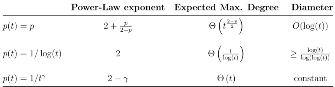
• The degree distribution follows a power law distribution with exponent which is a function of its parameterp given by β = 2 + 2−pp. Actually, this results may be found in [10], but we cite it here for completeness;
• The existence, with high probability, of a community whose order goes to infinity as the graph’s size increases. We specify the community’s order in function of the model’s parameter p. This result may be found in the preprint at http://arxiv.org/abs/ 1509.04650
• By a coupling with the classical Albert-Barabasi’s model we show that the model exhibits the small-world phenomenon;
The p(t)-model:
• The degree distribution follows a power law distribution with exponent which depends on how fast the function p(t) goes to zero;
In this Chapter we provide a rigorous analysis of a specific non-homogeneous random graph model, whose motivation was to combine scale-freeness and clustering. This model was introduced in 2001 by Holme and Kim [19]. The Holme-Kim or HK model describes a random sequence of graphs {Gt}t2N that will be formally defined in Section 2.2. Here is
an informal description of this evolution. Fix two parameters p 2 [0,1] and a positive integer m >1, and start with a graphG1. For t >1, the evolution fromGt−1 toGt consists
of the addition of a new vertex vt and mnew edges between vt and vertices already in Gt−1.
These m edges are added sequentially in the following fashion.
1. The first edge is always attached following thepreferential attachment (PA)mechanism, that is, it connects to a previously existing node w with probability proportional to the degree of w inGt−1.
2. Each of the m−1 remaining edges makes a random decision on how to attach.
(a) With probability p, the edge is attached according to the triad formation (TF)
mechanism. Letw0 be the node of Gt−1 to which the previous edge was attached. Then the current edge connects to a neighbor w of w0 chosen with probability
proportional to number of edges between wand w0.
(b) With probability 1−p (p2[0,1] fixed) the edge follows the same PA mechanism as the first edge (with fresh random choices).
The case p = 0 of this process, where only preferential attachment steps are performed, is essentially the Barab´asi- ´Albert model [3]. The triad formation steps, on the other hand, are reminiscent of the copying model by Kumar et al. [20]. Holme and Kim argued on the basis of simulations and non-rigorous analysis that their model has the properties of scale-freeness and positive clustering.
model has clustering admits two different answers depending on how we define clustering.
2.1
Definition of the process
In this section we give a more formal definition of the Holme-Kim process.
The model has two parameters: a positive integer numberm ≥2 and a real numberp2[0,1]. It produces a graph sequence{Gt}t≥1 which is obtained inductively according to the growth rule we describe below.
Initial state. The initial graph G1, which will be taken as the graph with vertex set
V1 ={1} and a single edge, which is a self-loop.
Evolution. Fort >1, obtainGt+1 fromGtadding to it a vertext+ 1 andmedges between
t+ 1 and vertices Yt(+1i) 2Vt, 1im. These vertices are chosen as follows. Let Ft be the
σ-field generated by all random choices made in our construction up to time t. Assume we are given i.i.d. random variables (⇠t(+1i) ) independent from Ft. We define:
P
⇣
Yt(1)+1 =u%% %Ft
⌘
= dt(u) 2mt,
which means the first choice of vertex is always made using the preferential attachment
mechanism. The next m−1 choices Yt(+1i), 2 i m, are made as follows: let F (i−1)
t be
the σ-field generated by Ft and all subsequent random choices made in choosing Yt(+1j) for 1j i−1. Then:
P
⇣
Yt(+1i) =u%% %⇠
(i)
t+1 =x,F (i−1)
t
⌘
=
8
> > > > > > <
> > > > > > :
dt(u)
2mt if x= 0,
et(Yt(+1i−1),u)
dt(Yt(+1i−1))
if x= 1 and u2Γt(Yt(+1i−1)),
0 otherwise.
In words, for each choice for them−1 end points, we flip an independent coin of parameterp
and decide according to it which mechanism we use to choose the end point. With probability
p use the triad formation mechanism, i.e., we choose the end point among the neighbors of the previously chosen vertex Yt(+1i−1). With probability 1−p, we make a fresh choice from Vt
using the preferential attachment mechanism. In this sense, if⇠t(i) = 1 we say we have taken
2.1.1
Our results
The main results in this Chapter show that such a disparity between local and global cluster-ing does indeed occur in the specific case of the Holme-Kim model, albeit in a less extreme form than what the Example suggests.
Theorem 2.1.1 (Positive local clustering for HK). Let {Gt}t≥0 be the sequence of graphs
generated by the Holme-Kim model with parameters m ≥2and p2(0,1). Then there exists
c >0 depending only on m and p such that the local clustering coefficientsCloc
Gt of the graphs
Gt satisfy:
lim
t!+1P
!
CGloct ≥c
"
= 1.
Theorem 2.1.2 (Vanishing glocal clustering for HK). Let {Gt}t≥0 be as in Theorem 2.1.1.
Then there exist constantsb1, b2 >0depending only onmandpsuch that the global clustering
coefficients CGglot satisfy:
lim
t!+1P
✓
b1 logt C
glo Gt
b2 logt
◆
= 1.
Thus for large t, one of the two clustering coefficients is typically far from 0, whereas the other one goes to 0 in probability, albeit at a small rate. This shows that the remark by Bollob´as and Riordan is very relevant in the analysis of at least one network model. Our results contradict the numerical findings of [27], where the Holme-Kim model is cited as a model that exhibits positive “clustering coefficient”, but the definition of clustering used corresponds to the global coefficient1.
For completeness, we will also check in the Appendix that the HK model is scale-free with power-law exponent β= 3. The proof follows from standard methods in the literature.
Theorem 2.1.3 (The power-law for HK). Let {Gt}t≥0 be as in the previous theorem. Also
let Nt(d) be the number of vertices of degree d in Gt and set
Dt(d) := E
Nt(d)
t .
Then
lim
t!1Dt(d) =
2(m+ 3)(m+ 1) (d+ 3)(d+ 2)(d+ 1).
and
P
⇣
|Nt(d)−Dt(d)t| ≥16d·c· p
t⌘(t+ 1)d−me−c2 .
1
2.1.2
Heuristics and a seemingly general phenomenon
The disparity betweenCloc G andC
glo
G should be ageneral phenomenon for large scale-free graph
models with many (but not too many triangles). This will transpire from the follwowing heuristic analysis of the Holme-Kim case with p2(0,1).
To begin, it is not hard to understand why Theorem 2.1.1 should be true. By Theorem 2.1.3, there is a positive fraction of nodes with degree m. Moreover, a positive fraction of these vertices are contained in at least one triangle because of TF steps. A more general observation may be made.
Reason for positive local clustering: if a positive fraction of nodes have degree d (assumed constant), and a positive fraction of these nodes are con-tained in at least one triangle, then the local clustering coefficient Cloc
Gt must be
bounded away from zero.
We now argue that the vanishing of CGglot should be a consequence of the power law degree
distribution. The global clustering coefficient CGglot is essentially the ratio of the number of
triangles to the number of cherries inGt, the latter being denoted byCt. Now, one can easily
show that the number of triangles inGt grows linearly int with high probability, so:
CGglot ⇡
# of triangles in Gt
Ct ⇡
t Ct
.
To estimateCt, we note that each vertexv of degreedinGtis the “middle vertex” of exactly
d(d−1)/2⇡d2 cherries. This means
Ct
t ⇡
t
X
d=1
Nt(d)
t d
2
⇣
Nt(d)
t ⇠Dt(d)⇡d
−3 by Theorem 2.1.3⌘ ⇡
t
X
d=1
1
d ⇡logt.
Our reasoning is not rigorous because it requires bounds onNt(d) for very larged. However, we feel our argument is compelling enough to be true for many models. In fact, considering the case where Nt(d)/t⇡d−β for 0< β 3, one is led to the following.
Heuristic reason for large number of cherries: if the fraction of nodes of degree d in Gt is ⇡ d−β for some 0 < β 3, the number of cherries Ct
is superlinear in t. More precisely, we expect Ct/t ⇡ t3−β for 0 < β < 3 and
The power law range 0 < β 3 corresponds to most models of large networks in the literature. Likewise, we believe that the disparity between CGglot and Cloc
Gt should hold for all
“natural” random graph sequences with many triangles and power law degree distribution with exponent 0< β 3. The general message is this.
Heuristic disparity between local and global clustering: achieving positive local clustering is “easy”: just introduce a density of triangles in sparse areas of the graph. On the other hand, if the number of triangles in Gt grows
linearly with time, and the fraction of nodes of degree d in Gt is ⇡d−β for some 0< β3, then one expects a vanishingly small global clustering coefficient.
2.1.3
Main technical ideas
At a high level, our proofs follow standard ideas from previous rigorous papers on complex networks. For instance, suppose one wants to keep track of the number of nodes of degree
d at time t, for d = m, m+ 1, . . . , D. Letting Nt = (Nt(m), . . . , Nt(D)), the basic strategy adopted in several previous papers is to find a deterministic matrixMt−1and a deterministic
vector rt−1, both measurable with respect to G0, . . . , Gt−1, such that:
Nt=Mt−1Nt+rt−1+✏t, where E(✏t |G0, . . . , Gt)⇡0.
This can be seen as “noisy version” of the deterministic recursion Nt = Mt−1Nt−1 +rt−1
with ✏t the “noise” term. One then studies the recursion and uses martingale techniques (especially the Azuma-H¨offding inequality) to prove thatNtconcentrates around the solution of the deterministic recursion. Our own proof of the degree power law follows this outline, and is only slightly different from the one in [11].
Theorem 2.1.4 (The Weak Law of large Numbers forCt). Let Ctbe the number of cherries
in Gt, then
Ct
tlogt
P −!
✓
m+ 1 2
◆
.
Overall, we believe our martingale analysis of Ct is our main technical contribution.
2.1.4
Organization.
The remainder of this Chapter is organized as follows. Section 2.2 presents a formal definition of the model. In Section 2.3 we prove technical estimates for the degree which will be useful throughout the Chapter. Sections 2.4 and 2.5 are devoted to prove the bounds for the local and the global clustering coefficients, respectively. Section 2.6 presents a comparative explanation for the so distinct behavior of the clustering coefficients. The proof of the power-law distribution is done at the end of the Chapter, in Section 2.7 because it follows well known martingale arguments.
2.2
Formal definition of the process
In this section we give a more formal definition of the Holme-Kim process (compare with the beginning of this Chapter).
The model has two parameters: a positive integer numberm ≥2 and a real numberp2[0,1]. It produces a graph sequence{Gt}t≥1 which is obtained inductively according to the growth
rule we describe below.
Initial state. The initial graph G1, which will be taken as the graph with vertex set
V1 ={1} and a single edge, which is a self-loop.
Evolution. Fort >1, obtainGt+1 fromGtadding to it a vertext+ 1 andmedges between
t+ 1 and vertices Yt(+1i) 2Vt, 1im. These vertices are chosen as follows. Let Ft be the
σ-field generated by all random choices made in our construction up to time t. Assume we are given i.i.d. random variables (⇠t(+1i) ) independent from Ft. We define:
P⇣Yt(1)+1 =u%% %Ft
⌘
= dt(u) 2mt,
which means the first choice of vertex is always made using the preferential attachment
the σ-field generated by Ft and all subsequent random choices made in choosing Yt(+1j) for 1j i−1. Then:
P
⇣
Yt(+1i) =u
% % %⇠
(i)
t+1 =x,F (i−1)
t
⌘
=
8
> > > > > > <
> > > > > > :
dt(u)
2mt if x= 0,
et(Yt(+1i−1),u)
dt(Yt(+1i−1))
if x= 1 and u2Γt(Yt(+1i−1)),
0 otherwise.
In words, for each choice for them−1 end points, we flip an independent coin of parameterp
and decide according to it which mechanism we use to choose the end point. With probability
p use the triad formation mechanism, i.e., we choose the end point among the neighbors of the previously chosen vertex Yt(+1i−1). With probability 1−p, we make a fresh choice from Vt using the preferential attachment mechanism. In this sense, if⇠t(i) = 1 we say we have taken a TF-step. Otherwise, we say aPA-step was performed.
2.3
Technical estimates for vertex degrees
In this section we collect several results on vertex degrees. Subsection 2.3.1 describes the probability of degree increments in a single step. In Subsection 2.3.2 we obtain upper bounds on all degrees. Some of these results are fairly technical and may be skipped in a first reading.
2.3.1
Degree increments
We begin the following simple lemma.
Lemma 2.3.1. For all k 2 {1, .., m}, there exists positive constants cm,p,k such that
P(∆dt(v) =k|Gt) = cm,p,k
dk t(v)
t +O
✓
dkt+1(v)
tk+1
◆
.
In particular, for k= 1 we have cm,p,1 = 1/2.
Proof. We begin proving the following claim involving the random variables Yt(i)
Claim: For all i2 {0,1,2, . . . , m},
P⇣Yt(+1i) =v%% %Gt
⌘
= dt(v)
Proof of the claim: The proof follows by induction on i. For i = 1 we have nothing to do. So, suppose the claim holds for all choices before i−1. Then,
P
⇣
Yt(+1i) =v
% % %Gt
⌘
=P
⇣
Yt(+1i) =v, Y (i−1)
t+1 =v
% % %Gt
⌘
+P
⇣
Yt(+1i) =v, Y (i−1)
t+1 6=v
% % %Gt
⌘
= (1−p) 4m2
d2
t(v)
t2 +P
⇣
Yt(+1i) =v, Y (i−1)
t+1 6=v
% % %Gt
⌘
.
(2.3.3)
For the first term on the r.h.s the only way we can choose v again is following a PA-step
and then choosingv according to preferential attachment rule. This means
P⇣Yt(+1i) =v, Yt(+1i−1) =v%% %Gt
⌘
= (1−p) 4m2
d2
t(v)
t2 . (2.3.4)
For the second term, we divide it in two sets, whether the vertex chosen at the previous choice is a neighbor of v or not.
P⇣Yt(+1i) =v, Yt(+1i−1) 6=v%% %Gt
⌘
= X u /2ΓGt(v)
P⇣Yt(+1i) =v, Yt+1(i−1) =u%% %Gt
⌘
+ X u2ΓGt(v)
P
⇣
Yt(+1i) =v, Y (i−1)
t+1 =u
% % %Gt
⌘
= (1−p)dt(v) 2mt
0
@ X
u /2ΓGt(v)
dt(u) 2mt 1 A +p 0 @ X
u2ΓGt(v)
eGt(u, v)
dt(u)
dt(u) 2mt
1
A
+(1−p) 2m
dt(v)
t
0
@ X
u2ΓGt(v)
dt(u) 2mt
1
A
= dt(v) 2mt −
(1−p) 4m2
d2
t(v)
t2 .
We used our inductive hypothesis and that
X
u2ΓGt(v)
dt(u) 2mt +
X
u /2ΓGt(v)
dt(u)
2mt = 1− dt(v)
2mt
Returning to (2.3.3) we prove the claim. ⌅
We will show the particular case k= 1 since we have particular interest in the value of cm,p,1
is by definition a homogeneous Markovian process. This means to evaluate the probability of a vertex increasing its degree by exactly one, the case k = 1, we just need to know the probabilities of transition. In this way, use the notationPtto denote the measure conditioned onGt and go to the computation of the probabilities of transition. We start by the hardest one.
Pt
⇣
Yt(+1i+1) =v%% %Y
(i)
t+1 6=v
⌘
= X u2ΓGt(v)
Pt
⇣
Yt(+1i+1) =v%% %Y
(i)
t+1 =u
⌘
Pt
⇣
Yt(+1i) =u%% %Y
(i)
t+1 6=v
⌘
+ X u /2ΓGt(v)
Pt⇣Yt(+1i+1) =v%% %Y
(i)
t+1 =u
⌘
Pt⇣Yt(+1i) =u%% %Y
(i)
t+1 6=v
⌘
(2.3.5)
When u 2 ΓGt(v), we can choose v taking any of the two steps. This implies the equation
below
Pt
⇣
Yt(+1i+1) =v%% %Y
(i)
t+1=u
⌘
= (1−p)dt(v) 2mt +p
et(u, v)
dt(u) , (2.3.6)
but when u /2 ΓGt(v) the only way we can choose v is following a PA-step, which implies
that
Pt⇣Yt(+1i+1) =v%% %Y
(i)
t+1 =u
⌘
= (1−p)dt(v)
2mt. (2.3.7)
We also notice that the equation below holds, since u6=v and our claim is true
Pt
⇣
Yt(+1i) =u
% % %Y
(i)
t+1 6=v
⌘
= Pt
⇣
Yt(+1i) =u⌘
Pt⇣Yt(+1i) 6=v⌘
Claim
= dt(u)
2mtPt⇣Yt(+1i) 6=v⌘. (2.3.8)
And the same Claim also implies that 1
Pt
⇣
Yt(+1i) 6=v⌘
= 1 1−dt(v)
2mt
= 1 +
1
X
n=1
✓
dt(v) 2mt
◆n
. (2.3.9)
Combining the last three equations to (2.3.5), we are able to get
Pt
⇣
Yt(+1i+1) =v%% %Y
(i)
t+1 6=v
⌘
= (1−p)dt(v) 2mt +p
dt(v) 2mt 1 +
1
X
n=1
✓
dt(v) 2mt
◆n!
= dt(v) 2mt +O
✓
d2
t(v)
t2
◆
.
If we chose v at the previous choice, the only way we select it again is following a PA-step, this means that
Pt
⇣
Yt(+1i+1) =v%% %Y
(i)
t+1 =v
⌘
= (1−p)dt(v)
2mt. (2.3.11)
From these two probabilities of transition we may obtain the other ones.
To compute the probability of {∆dt(v) = 1} given Gt we may split it in m possible ways to increase dt(v) by exactly one. Each possible way has an index i 2 {1, ..., m} meaning the step we chosev and then we must avoid it at the other m−1 choices. This means that each of these m ways has a probability similar to the expression below
✓
1− dt(v) 2mt −O
✓
d2
t(v)
t2
◆◆i−1✓
dt(v) 2mt +O
✓
d2
t(v)
t2
◆◆ ✓
1− dt(v) 2mt −O
✓
d2
t(v)
t2
◆◆m−i
which implies that
P(∆dt(v) = 1|Gt) = dt(v) 2t +O
✓
d2
t(v)
t2
◆
.
The casesk > 1 are obtained in the same way, considering the!m
k
"
ways of increase dt(v) by
k.
Observation 1. We must notice that term O⇣dkt+1(v)
tk+1
⌘
given by the Lemma actually is a statement stronger than the real big-O notation. Since the Lemma’s proof implies the existence of a positive constant ˜cm,p,k such that
O
✓
dkt+1(v)
tk+1
◆
c˜m,p,k
dkt+1(v)
tk+1 ,
for all vertex v and time t.
2.3.2
Upper bounds on vertex degrees
To control the number of cherries, Ct, we will need upper bounds on vertex degrees. The bound is obtained applying the Azuma-Hoffding inequality to the degree of each vertex, which is a martingale after normalizing by the quantity defined below.
φ(t) := t−1
Y
s=1
✓
1 + 1 2s
◆
. (2.3.12)
A fact about φ(t) will be useful: there exists positive constants b1 and b2 such that
b1
p
tφ(t)b2
p
t,
Proposition 2.3.13. For each vertex j, the sequence (Xt(j))t≥j defined as
Xt(j) :=
dt(j)
φ(t)
is a martingale.
Proof. Since the vertex j will remain fixed throughout the proof, we will write simply Xt instead of Xt(j).
Observe that we can writedt+1(j) as follows
dt+1(j) = dt(j) +
m
X
k=1
1
n
Yt(+1k) =jo.
In addition, we proved in Lemma 2.3.1 that, for all k 21, ..., m, we have
P
⇣
Yt(+1k) =j%% %Gt
⌘
= dt(j)
2mt. (2.3.14)
Thus, the follow equivalence relation is true
E[dt+1(j)|Gt] =
✓
1 + 1 2t
◆
dt(j). (2.3.15)
Then, dividing the above equation by φ(t+ 1) the desired result follows.
Once we have Proposition 2.3.13 we are able to obtain an upper bound for dt(j).
Theorem 2.3.16. There is a positive constant b3 such that, for all vertex j
P⇣dt(j)≥b3
p
tlog(t)⌘t−100.
Proof. The proof is essentially applying Azuma’s inequality to the martingale we obtained in Proposition 2.3.13. Again we will write it as Xt.
Applying Azuma’s inequality demands controlling Xt’s variation, which satisfies the upper bound below
|∆Xs|=
% % % % %
ds+1(j)−
!
1 + 21s"
ds(j)
φ(s+ 1)
% % % % %
2m
φ(s+ 1)
b4
p
s. (2.3.17)
Thus,
t
X
s=j+1
We must notice that none of the above constants depend on j. Then, Azuma’s inequality gives us that
P(|Xt−X0|> λ)2 exp
⇢
− λ
2
b5log(t)
8
. (2.3.18)
Choosing λ= 10pb5log(t) and recalling Xt=dt(j)/φ(t) we obtain
P
✓% % % %
dt(j)− mφ(t)
φ(j)
% % % %
>10pb5φ(t) log(t)
◆
t−100.
Finally, using that b1
p
tφ(t+ 1) b2
p
t, comes
P
✓% % %
%dt(j)−
mφ(t)
φ(j)
% % % %>10
p
b5b2
p
tlog(t)
◆
t−100.
Implying the desired result.
An immediate consequence of Theorem 2.3.16 is an upper bound for the maximum degree of Gt
Corollary 2.3.19 (Upper Bound to the maximum degree). There exists a positive constant
b1 such that
P⇣dmax(Gt)≥b1
p
tlog(t)⌘t−99.
Proof. The event involving dmax(Gt) may be seen as follows
n
dmax(Gt)≥b1
p
tlog(t)o=[ jt
n
dt(j)≥b1
p
tlog(t)o.
Using union bound and applying Theorem 2.3.16 we prove the Corollary.
The next three lemmas are of a technical nature. Their statements will become clearer in the proof of the upper bound for Ct.
Lemma 2.3.20. There are positive constants b6 and b7, such that, for all vertex j and all
time t0 t, we have
P dt0(j)> b4
r
t0
tdt(j) +b5
p
t0log(t)
!
t−100.
Proof. For each vertex j and t0 t, consider the sequence of random variables (Zs)s≥0
Concerning Zs’s variation, using (2.3.17), we have the following upper bound
|∆Zs|=|∆Xt0+s| b4
p
t0+s
.
Thus,
t−t0
X
s=0
|∆Zs|2 b5log(t).
Applying Azuma’s inequality, we obtain
P(|Zt−t0 −Z0| ≥λ)2 exp
⇢
− λ
2
b5log(t)
8
. (2.3.21)
But, the definition of Zs and the fact that φ(t) = Θ
!p
t"
the inclusion of events below is true
⇢
dt0(j)> b2
p
t0λ+
b2pt0
b1
p
tdt(j)
8
⇢ {|Zt−Z0| ≥λ},
which, combined to (2.3.21), proves the lemma if we choose λ= 10pb5log(t).
Lemma 2.3.22. There is a positive constant b8 such that
P t
[
j=1
t
[
t0=j
<
dt0(j)> b8
p
t0log(t)
!
2t−98.
Proof. This Lemma is consequence of Theorem 2.3.16 and Lemma 2.3.20, which state, re-spectively
P
⇣
dt(j)≥b3
p
tlog(t)⌘t−100, (2.3.23)
P dt0(j)> b4
r
t0
tdt(j) +b5
p
t0log(t)
!
t−100. (2.3.24)
In which the constants b3, b4 and b5 don’t depend on the vertexj neither the times t0 and t.
Now, for each t0 t and vertex j, consider the events below
At0,j :=
<
dt0(j)> b8
p
t0log(t) ,
Bt0,j :=
(
dt0(j)> b4
r
t0
t dt(j) +b5
p
t0log(t)
)
,
e
Ct,j :=
n
dt(j)≥b3
p
Now we obtain an upper bound for P(At0,j) using the bounds we have obtained for the
probabilities of Bt0,j and Ct,j.
P(At0,j) = P(At0,j\Bt0,j) +P
!
At0,j\B
c t0,j
"
P(Bt0,j) +P
!
At0,j\B
c
t0,j\Ct,j
"
+P!At0,j\B
c t0,j\C
c t,j
"
P(Bt0,j) +P(Ct0,j) +P
!
At0,j\B
c t0,j\C
c t,j
"
.
(2.3.25)
However, notice we have the following inclusion of events
Btc0,j\Ct,jc ⇢<
dt0(j)(b4b3+b5)
p
t0log(t) .
Thus, choosingb8 = 2(b4b3+b5) we haveAt0,j\B
c t0,j\C
c
t,j =;, which allows us to conclude that
P(At0,j)2t
−100.
Finally, an union bound over t0 followed by a union bound over j implies the desired result.
2.4
Positive local clustering
In this section we prove Theorem 2.1.1, which says that the local clustering coefficient is bounded away from 0 with high probability.
Proof of Theorem 2.1.1. We must find a lower bound for Cloc
Gt :=
1
t
X
v2Gt
CGt(v).
Let vm be a vertex in Gt whose degree is m. Observe that each TF-step we took when vm was added increase e(ΓGt(vm)) by one. So, denote by Tv the number of TF-steps taken at
the moment of creation of vertex v. Since all the choices of steps are made independently,
Tv follows a binomial distribution with parameters m−1 and p. Now, for every vertex we add to the graph, put a blue label on it if Tv ≥ 1. The probability of labeling a vertex is bounded away from zero and we denote it by pb.
By Theorem 2.1.3, with probability at least 1−t−100, we have
Nt(m)≥b1t−b2
p
tlog(t).
Thus, the number of vertices in Gt of degree m which were labeled, Nt(b)(m), is bounded from below by a binomial random variable, Bt, with parameters b1t−b2
p
tlog(t) and pb. But, about Bt we have, for allδ >0,
P
✓
Bt E [Bt]
4
◆
!
1−pb+pbe−δ
"b1t−b2ptlog(t)
expnδpb
⇣
b1t−b2
p
and choosingδ properly we conclude that, w.h.p,
Nt(b)(m)≥pb
⇣
b1t−b2
p
tlog(t)⌘/4. (2.4.1)
Finally, note that each blue vertex of degree m has CGt(v) > 2m
−2. Combining this with
(2.4.1) we have
Cloc Gt >
1
t
X
v2Nt(b)(m)
CGt(v)> t
−1N(b)
t (m)2m−2
> t−12m−2pb
⇣
b1t−b2
p
tlog(t)⌘/4
!2m−2p
bb1 >0 as t !+1,
proving the theorem.
2.5
Vanishing global clustering
This section is devoted to the proof of Theorem 2.1.2 which states that the global clustering of Gt goes to zero at 1/logt speed. Since the proof depends on estimates for the number of cherries, Ct, we first derive the necessary bounds and finally put all the pieces together at the end of this section.
2.5.1
Preliminary estimates for number of cherries
Let
˜
Ct:= t
X
j=1
d2t(j)
denote the sum of the squares of degrees in Gt. We will to prove bounds for ˜Ct instead of proving them directly for Ct. Since Ct = ˜Ct/2−mt the results obtained for ˜Ct directly extend to Ct.
Lemma 2.5.1. There is a positive constant B3 such that
E
⇣
˜
Cs+1−C˜s
⌘2% % % %
Gs
A
B3
dmax(Gs) ˜Cs
Proof. We start the proof noticing that for all vertexj we haved2
s+1(j)−d2s(j)2mds(j)+m2 deterministically From this remark the inequality below follows.
˜
Cs+1−C˜s 2m s
X
j=1
ds(j)1{∆ds(j)≥1}+ 2m2. (2.5.2)
Since all vertices have degree at leastm, we have m2 mPs
j=1ds(j)1{∆ds(j)≥1}, thus
˜
Cs+1−C˜s 4m s
X
j=1
ds(j)1{∆ds(j)≥1}. (2.5.3)
Applying Cauchy-Schwarz to the above inequality, we obtain
⇣
˜
Cs+1−C˜s
⌘2
16m2
s
X
j=1
ds(j)1{∆ds(j)≥1} ·1{∆ds(j)≥1}
!2
16m2
s
X
j=1
d2s(j)1{∆ds(j)≥1}
! s
X
j=1
1{∆ds(j)≥1}
!
16m3
s
X
j=1
d2s(j)1{∆ds(j)≥1}.
(2.5.4)
Recalling that
P(∆ds(j)≥1|Gs) ds(j) 2s
we have
E
✓ ⇣
˜
Cs+1−C˜s
⌘2% % % %
Gs
◆
B3
s
X
j=1
d3
s(j)
s B3
dmax(Gs) ˜Cs
s ,
concluding the proof.
Theorem 2.5.5 (Upper bound forCt). There is a positive constant B1 such that
P!Ct≥B1tlog2(t)
"
t−98.
Proof. We show the result for ˜Ct, which is greater than Ct. To do this, we need to deter-mine E[d2
t+1(j)|Gt].
As in proof of Proposition 2.3.13, write
dt+1(j) = dt(j) +
m
X
k=1
1
n
and denote Pm
k=11
n
Yt(+1k) =jo by∆dt(j). Thus,
d2
t+1(j) =d2t(j)
✓
1 + ∆dt(j)
dt(j)
◆2
=d2
t(j) + 2dt(j)∆dt(j) + (∆dt(j))2.
Combining the above equation with (2.3.14) and (2.3.15), we get
E⇥d2t+1(j)%%Gt ⇤
=d2t(j) + d
2
t(j)
t +E
⇥
(∆dt(j))2%%Gt ⇤
. (2.5.6)
Dividing the above equation by t+ 1, we get
E
d2
t+1(j)
t+ 1
% % % %Gt
A
= d
2
t(j)
t +
E[(∆dt(j))2|Gt]
t+ 1 , (2.5.7)
which implies
E
"
˜
Ct+1
t+ 1
% % % % % Gt #
= C˜t
t + m2
t+ 1 + t
X
j=1
E[(∆dt(j))2|Gt]
t+ 1 . (2.5.8)
It is straightforward to see that ∆dt(j)(∆dt(j))2 m∆dt(j), which implies
E⇥(∆dt(j))2% %Gt
⇤
=Θ
✓
dt(j)
t
◆
.
Thus, (2.5.8) may be written as
E
"
˜
Ct+1
t+ 1
% % % % % Gt #
= C˜t
t +Θ
✓ 1 t ◆ . (2.5.9) Now, define
Xt:= ˜
Ct+1
t+ 1.
Equation (2.5.9) states thatXtis a martingale up to a term of magnitude Θ
!1
t
"
. In order to apply martingale concentration inequalities, we decompose Xt as in Doob’s Decomposition theorem. Xt can be written as Xt = Mt +At, in which Mt is a martingale and At is a predictable process. By Equation (2.5.9), we have
At= t
X
s=2
E[Xs|Gs−1]−Xs−1 =
t X s=2 Θ ✓ 1 s ◆ . (2.5.10)
The remainder of the proof is devoted to controllingXt’s martingale component using Freed-man’s Inequality. Once again, by Doob’s Decomposition Theorem, we have
Mt:=X0+
t
X
s=2
Xs−E[Xs|Gs−1].
Observe thatMt+1 =Mt+Xt+1−E[Xt+1|Gt], thus
|∆Ms|=|Xs+1−E[Xs+1|Gs]| |Xs+1−Xs|+
b9 s % % % % % ˜
Cs+1−
!
1 + 1s" ˜
Cs
s+ 1
% % % % %
+ b9
s
b10
dmax(Gs)
s +b11
˜
Cs
s2 +
b9
s.
(2.5.11)
Since∆C˜s attains its maximum when the vertices of maximum degree in Gs receive at least a new edge at time s+ 1. Furthermore, since dmax(Gs)msand ˜Cs m2s2, there exists a constant b12 such that maxst|∆Ms| b12 almost surely.
Combining
|∆Ms|
% % % % % ˜
Cs+1−
!
1 + 1
s
" ˜
Cs
s+ 1
% % % % %
+ b9
s
with Cauchy-Schwarz and Lemma 2.5.1, we obtain positive constants b13, b14 and b15 such
that
E⇥(∆Ms)2%%Gs ⇤ CS
b13
E
h
(∆C˜s)2%% %Gs
i
s2 +b14
˜
C2
s
s4 +
b15
s2
Lemma2.5.1
b16
dmax(Gs) ˜Cs
s3 +b14
˜
C2
s
s4 +
b15
s2.
(2.5.12)
Now, define Vt as
Vt:= t
X
s=2
E⇥(∆Ms)2% %Gs
⇤
and call bad set the event below
Bt:= t
[
j=1
t
[
t0=j
<
dt0(j)> b8
p
t0log(t) ,
Also notice that ˜Cs b17dmax(Gs)salmost surely and in Btc we have dmax(Gs)b8pslog(t)
for all st. Then, outside Bt we have
Vt
(2.5.12)
t
X
s=2
b16
dmax(Gs) ˜Cs
s3 +b14
˜
C2
s
s4 +
b15 s2 t X s=2
b16b28b17s2log2(t)
s3 +
b14b217s3log2(t)
s4 +
b15
s2
b18log3(t).
(2.5.13)
So, by Freedman’s inequality, we obtain
P!Mt> λ, Vtb18log3(t)
"
exp
⇢
− λ
2
2b18log3(t) + 2b12λ/3
8
.
Therefore, ifλ =b19log2(t) with b19 large enough, we get
P!Mt > b19log2(t), Vtb18log3(t)
"
t−100. (2.5.14) The inequality (2.5.13) guarantees the following inclusion of events
Btc ⇢<
Vtb18log3(t) . (2.5.15)
And also,
<
Xt≥b21log2(t) ⇢
<
Mt≥(b21−b20) log2(t) . (2.5.16)
since Atb20log(t) and Mt≥Xt−b20log(t).
Finally,
P!Mt > b19log2(t)
"
=P!Mt> b19log2(t), Vtb18log3(t)
"
+P!Mt> b19log2(t), Vt > b18log3(t)
"
t−100+P(Bt) P!Mt > b19log2(t)
"
3t−98,
proving the Theorem..
We notice that from equation (2.5.8) we may extract the recurrence below
E h ˜ Ct i = ✓
1 + 1
t−1
◆
E
h
˜
Ct−1
i
+c0,
in which c0 is a positive constant depending on m and p only. Expanding it, we obtain
E h ˜ Ct i = t−1
Y
s=1
✓
1 + 1
s ◆ E h ˜ C1 i
+c0
t−1
X
s=1
t−1
Y
r=s
✓
1 + 1
r
◆
,
2.5.2
The bootstrap argument
Obtaining bounds for Ct requires some control of its quadratic variation, which requires bounds for the maximum degree and Ct, as in Lemma 2.5.1. Applying some deterministic bounds and upper bounds on the maximum degree we were able to derive an upper bound for Ct, which is of order E[Ct] logt. To improve this bound and obtain the right order, we proceed as in proof of Theorem 2.5.5, but making use of the preliminary estimatejust discussed. This is what we call the bootstrap argument.
The result we obtain is enunciated in Theorem 2.1.4 and consist of a Weak Law of Large Numbers, which states that Ct divided by tlogt actually converges in probability to a con-stant depending only on m.
Proof of Theorem 2.1.4. In proof of Theorem 2.5.5, we decomposed the process Xt = ˜Ct/t in two components: Mt and At. The first part of the proof will be dedicated to showing that Mt=o(log(t)),w.h.p. Then we show that At= (m2+m) log(t) also w.h.p.
We repeat the proof given for Theorem 2.5.5, but this time we change our definition of bad set to
Bt = t
[
s=log1/2(t)
n
˜
Cs≥b20slog2(s)
o
.
By Theorem 2.5.5 and union bound, P(Bt)log−97/2(t). Observe that an upper bound for ˜
Cs gives an upper bound for dmax(Gs), since
d2max(Gs)C˜s =) dmax(Gs)
q
˜
Cs =) dmax(Gs)pslog(s),
when ˜Cs slog2(s).
Using (2.5.12) we have, inBc t,
Vt t−1
X
s=1
b16
dmax(Gs) ˜Cs
s3 +b14
˜
Cs
2
s4 +
b14
s2
log1/2(t)−1
X
s=1
b016+ t−1
X
s=log1/2(t) b17
p
slog(s)slog2(s)
s3 +b18
s2log4(s)
s4 +
b14
s2
b19log1/2(t),
(2.5.17)
since dmax(Gs)m·s and ˜Cs 2m2·s2 for all s and, in Btc, dmax(Gs) p
b20slog(s) and
˜
Csb20slog2(s) for all s≥log1/2(t). Then, by Freedman’s inequality,
P⇣Mt ≥log1/4+δ(t), Vtb19log1/2(t)
⌘
Recall equation (2.5.8)
E
"
˜
Ct+1
t+ 1
% % % % % Gt #
= C˜t
t + m2
t+ 1 + t
X
j=1
E[(∆dt(j))2|Gt]
t+ 1 .
Now, we recall from Lemma 2.3.1 that for all k 2 {1, ..., m}
P
⇣
Yt(+1k)=v%% %Gt
⌘
= dt(v) 2mt.
Furthermore,
P⇣Yt(+1k) =v, Yt(+1j) =v%% %Gt
⌘
=O
✓
d2
t(v)
t2
◆
.
Thus,
E⇥(∆dt(v))2%%Gt ⇤
= dt(v) 2t +O
✓
d2
t(v)
t2
◆
, (2.5.19)
which implies that
E
"
˜
Ct+1
t+ 1
% % % % % Gt #
= C˜t
t +
m2+m
t+ 1 +O ˜ Ct t3 ! , and consequently
At = t
X
s=2
m2+m
s+ 1 +O ˜
Cs
s3
!
.
As we have already noticed before, all the constants involved in the big-O notation do not depend on the time or the vertex. From the above equation we deduce that, in Bc
t,
t
X
s=2
O C˜s s3
!
b11
log1/2(t)
X
s=2
˜
Cs
s3 +
t
X
s=log1/2(t)
slog2(s)
s3 b12log(log(t)).
Thus, in Bc t,
At= (m2+m) log(t) +o(log(t)).
Finally, fix a small positive "
P % % % % % ˜ Ct
tlog(t) −m
2+m
% % % % % > " ! =P ✓% % % %
Mt+At log(t) −m
2+m
% % % % > " ◆ P ✓% % % %
Mt+At log(t) −m
2+m
% % %
%> ", B
c t
◆
+P(Bt).
We also have that Bc
t ⇢ {Vtb19log1/2(t)}, which, combined to (2.5.18), implies
P
✓% % % %
Mt+At log(t) −m
2+m
% % %
%> ", Mt ≥log
1/4+δ (t), Btc
◆
=o(1).
And recall that, in Bc
t, Mt is at most log1/4+δ(t) and At= (m2+m) log(t) +o(log(t)), thus
P
✓% % % %
Mt+At log(t) −m
2+m
% % %
%> ", Mt<log
1/4+δ (t), Btc
◆
= 0
for large enough t.
Recalling that Ct= ˜Ct/2−mt we obtain the desired result.
2.5.3
Wrapping up
Until here we devoted our efforts to properly control the number of cherries inGt. Now, we combine these results with simple bounds for the number of triangles inGt to finally obtain the exact order of the global clustering.
Proof of Theorem 2.1.2. By Theorem 2.1.4 we have
Ct= Θ (tlog(t)),w.h.p.
But, observe that number of triangles inGt, ∆Gt, is bounded from above by
!m
2
"
t. And note that every TF-step we take increases ∆Gt by one. Then,
∆Gt ≥Zt=
t
X
s=1
Ts
whereTsis the number ofTF-steps we took at times. Since all the choices concerning which kind of step we follow are independent, Ts ⇠ bin(m−1, p) and Zt ⇠ bin((m−1)t, p). By Chernoff Bounds, Zt≥δ(m−1)pt, for a small δ, w.h.p. Thus,
∆Gt =Θ(t),w.h.p,
which conclude the proof.
2.6
Final comments on clustering
We end our discussion about clustering by comparing the two clustering coefficients from a different perspective than in Section 2.1.2. Recall thatCloc
clustering coefficients.
CGloct :=
1
t
X
v2Gt
CGt(v).
On the other hand, CGglot is a weighted average, where the weight of vertex v is the number of cherries that it belongs to,
CGglot = 3⇥
P
v2GtCGt(v)
!dt(v)
2
"
P
v2Gt
!dt(v)
2
" (2.6.1)
Thus the weight ofv inCGglot is basically proportional to the square of the degree. This skews
the distribution of weights towards high-degree nodes. The clustering of the high degree vertices is the reason why the two coefficients present so distinct behavior.
We will show below thatCGt(v) for a vertexv of high degreedis of orderd
−1, which explains
why CGglot goes to zero. Recall that the r.v. et(Γv) counts the number of edges between the neighbors ofv. Due to the definition of our model, one can only increseet(Γv) by one ifdt(v) is also increased by at least one unit. Sinceet(Γv) can only increase by munits in each time step, we have:
et(Γv)m dt(v),
which implies an upper bound for CGt(v)⇡ et(Γv)/dt(v)2 of order d
−1
t (v). The next propo-sition gives a lower bound of the same order.
Proposition 2.6.2. Let v be a vertex of Gt. Then, there are positive constants, b1 and b2,
such that
P
✓
CGt(v)
b1
dt(v)
% % % %
dt(v)≥b2log(t)
◆
t−100.
This proposition does not prove our clustering estimates, but seems interesting in any case.
Proof of the Proposition. Observe that if we choose v and take a TF-step thereafter, we increase et(Γv) by one. Then, if we look only at times in which this occurs, et(Γv) must be greater than a binomial random variable with parameters: number of times we choose v at the first choice and p. Since all the choices concerning the kind of step we take are made independently of the whole process, we just need to prove thatnumber of times we choose v
at the first choice, denoted by d(1)t (v), is proportional to dt(v) w.h.p.
Recall that Ys(1) indicates the vertex chosen at time s at the first of our m choices. The random variable d(1)t (v) can be written in terms of Y(1)’s just as follows
d(1)t (v) = t
X
s=v+1
We first claim that if dt(v) is large enough, a positive fraction of its value must come fromd(1)t (v).
Claim: There exists positive constants b1 and b2 such that
P
⇣
d(1)t (v)b1dt(v)
% %
%dt(v)≥b2log(t) ⌘
t−100.
Proof of the claim: To prove the claim we condition on all possible trajectories of dt(v). In this direction, let ! be an event describing whenv was chosen and how many times at each step. We have to notice that ! does not record whether v was chosen by a PA-step or a
TF-step. The event ! can be regarded as a vector in {0,1, ..., m}t−v−1 such that !(s) = k
means we chose v k-times at time s. For each !, let d!(v) be the degree of v obtained by the sequence of choices given by !.
Recall the Equations (2.3.10) and (2.3.11) which states that
Pt
⇣
Yt(+1i+1) =v%% %Y
(i)
t+1 6=v
⌘
= dt(v) 2mt +O
✓
d2
t(v)
t2
◆
and
Pt
⇣
Yt(+1i+1) =v
% % %Y
(i)
t+1 =v
⌘
= (1−p)dt(v) 2mt.
For any ! such that !(s) = k ≥ 1, we may show, using (2.3.10) and (2.3.11), that there exists a positive constant δ depending only on m and p, such that
P!Ys(1) =v%%! "
≥δ. (2.6.4)
Furthermore, given !, the random variables 1{Ys(1) = v} are independent. This implies that, given !, the random variabled(1)t (v) dominates stochastically another random variable following a binomial distribution of parameters d!(v)/m and δ. Thus, by Chernoff bounds, we can choose a small b1 such that
P
⇣
d(1)t (v)b1d!(v)
% % %!
⌘
exp (−d!(v)).
Since we are on the event Dt := {dt(v) ≥ b2log(t)}, all d!(v) ≥ b2log(t) for some b2 that
can be chosen in a way such that
P
⇣
d(1)t b1d!(v)
% % %!
⌘
t−100
for all ! compatible with Dt. Finally, to estimate nd(1)t (v)b1dt(v)
o
, we condition on all possible history of choices !
P⇣d(1)t (v)b1dt(v)
% % %Dt
⌘
=X !
P⇣d(1)t (v)b1dt(v)
% % %!, Dt
⌘
and this proves the claim. ⌅
As we observed at the beginning, et(Γv) dominates a random variable bin(d(1)t (v), p). And by the claim, d(1)t (v) is proportional to dt(v), w.h.p. Using Chernoff Bounds, we obtain the result.
2.7
Power law degree distribution
We end this Chapter by proving the power law distribution.
Lemma 2.7.1 (Lemma 3.1 [11]). Let at be a sequence of positive real numbers satisfying the
following recurrence relation
at+1 =
✓
1− bt
t
◆
at+ct.
Furthermore, suppose bt !b >0 and ct !c, then lim
t!1
at
t = c
1 +b.
Proof of Theorem 2.1.3. We divide the proof into two parts. Part (a) is the power law for the expected value of the proportion of vertices with degreed. Part (b) is the concentration inequalities Nt(d).
Proof of part (a).The is essentially the same gave in Section 3.2 of [11]. The key step is obtain a recurrence relation involving E[Nt(d)] which has the same form of that required by Lemma 5.1.1. To obtain the recurrence relation, observe that Nt+1(d) can be written as
follow
Nt+1(d) =
X
v2Nt(d)
{∆dt(v)=0}+
X
v2Nt(d−1)
{∆dt(v)=1}+. . .+
X
v2Nt(d−m)
{∆dt(v)=m}. (2.7.2)
Taking the conditional expected value with respect to Gt on the above equation, applying Lemma 2.3.1 and recalling that Nt(d)t, we obtain
E[Nt+1(d)|Gt] =Nt(d)
1− d 2t +O
✓
d2
t2
◆A
+Nt(d−1)
(d−1) 2t +O
✓
(d−1)2
t2 ◆A +O ✓ 1 t ◆ .
Finally, taking the expected value on both sides, denoting ENt(d) by a(td), we have
a(t+1d) =
2
41−
d
2 +O
⇣ d2 t ⌘ t 3 5a
(d)
t +a
(d−1)
t
2
4
d−1 2 +O
⇣
(d−1)2
t
⌘
t
3
5+O
✓
1
t
◆
From here, the proof follows by an induction on d ≥ m and application of Lemma 5.1.1, assuming ENt(d−1)
t −!Dd−1, which gives us
at(d)
t −!
Dd−1(d−21)
1 +d/2 =Dd−1
d−1
2 +d =:Dd
and this gives us that
Dd= 2 2 +m
d
Y
k=m+1
(k−1)
k+ 2 =
2(m+ 3)(m+ 1) (d+ 3)(d+ 2)(d+ 1)
which proves the part (a).
Proof of part (b). The proof is in line with proof of Theorem 3.2 in [11]. For this reason we show only that following process
Xt(d):=
Nt(d)−Ddt+ 16d·c· p
t
d(t) ,
in which d(t) is defined as
d(t) := t−1
Y
s=d
✓
1− d 2s
◆
is a submartingale and we give an upper bound for its variation.
As in Theorem 3.2 of [11], the proof follows by induction ond.
Inductive step: Suppose that for all d0 d−1 we have P⇣Nt(d0)Dd0t−16d0·c·
p
t⌘(t+ 1)d0−me−c2. (2.7.4)
Recalling that
E[Nt+1(d)|Gt] =
✓
1− d 2t +O
✓
d2
t2
◆◆
Nt(d) + (d−1)Nt(d−1) 2t +O
!
t−1"
we have the following recurrence relation
E
h
d(t+ 1)Xt(d)
% % %Gt
i
≥
✓
1− d 2t
◆
Nt(d) + (d−1)Nt(d−1) 2t
+O!
t−1"
+ 16d·c·pt−Dd(t+ 1).
(2.7.5)
The inductive hypothesis assure us that
Nt(d−1)≥Dd−1t−16(d−1)·c·
p
with probability at least 1−(t+ 1)d−1−me−c2
. Thus, returning on (2.7.5),
Eh d(t+ 1)Xt(d)%% %Gt
i
≥
✓
1− d 2t
◆
Nt(d)
+(d−1)Dd−1
2 −Dd(t+ 1) + 16d·c· p
t+O!
t−1"
.
(2.7.6)
But, observe that about the r.h.s of the above inequality, we have (d−1)Dd−1
2 −Dd(t+ 1) + 16d·c· p
t+O!
t−1"
≥
✓
1− d 2t
◆ ⇣
−Ddt+ 16d·c· p
t⌘
() (d−1)Dd−1
2 −Dd+O
!
t−1"
≥ dDd 2t −
8d2c
p
t
() (d−1)Dd−1
2 + 8d2c
p
t +O
!
t−1"
≥Dd+
dDd 2t
(2.7.7)
but the last inequality is true since we have (d−1)Dd−1 = (d+2)DdandDd= (d2(+3)(m+3)(d+2)(m+1)d+1). Returning to (2.7.6), we just proved that Xt(+1d) is a submartingale with fail probability bounded from above by (t+ 1)d−me−c2
. And its variation ∆Xt(d) satisfies the upper bound below
% %∆Xs(d)
% %
∆Ns(d) +Dd+ 16dcs−1/2 +dNs(d)(2s)−1 d(s+ 1)
m+ 2/(d+ 2) + 17dcs
−1/2+d/2
d(s+ 1)
2d
d(s+ 1) +
17dc
p
s d(s+ 1),
(2.7.8)
since ∆Ns(d) m, Ns(d)s and Dd 2/(d+ 2) for all s and d. Thus, there is a positive constant M, such that
% %∆Xs(d)
% %
2
16d
2 2
d(s+ 1)
+ M d
2c2
s 2
d(s+ 1)
. (2.7.9)
The lower bound for Nt(d) is proven applying Theorem 2.36 of [11] on Xt(d), setting
λ= 2c·
v u u t t+1 X
s=d
% % %∆X
(d)
The upper bound is obtained the same way, but considering the process
−X(d)
t :=
Nt(d)−Ddt−16d·c· p
t
d(t) ,