Formulation space search approach for the teacher/class timetabling problem

DOI: 10.2298/YUJOR0801001K

FORMULATION SPACE SEARCH APPROACH FOR THE

TEACHER/CLASS TIMETABLING PROBLEM

Yuri KOCHETOV

, Polina KONONOVA

, Mikhail PASCHENKO

Sobolev Institute of Mathematics, Russia 2

Novosibirsk State University, Russia

Received: March 2007 / Accepted: February 2008

Abstract: We consider the well known NP–hard teacher/class timetabling problem. Variable neighborhood search andtabu search heuristics are developed based on idea of the Formulation Space Search approach. Two types of solution representation are used in the heuristics. For each representation we consider two families of neighborhoods. The first family uses swapping of time periods for teacher (class) timetable. The second family bases on the idea of large Kernighan-Lin neighborhoods. Computation results for difficult random test instances show high efficiency of the proposed approach.

Keywords: _Timetable design, metaheuristics, local search, FSS approach. 1. INTRODUCTION

In this paper we consider the teacher/class timetabling problem for the Specialized Physical–Mathematical School which is a part of the Novosibirsk State University. All students in this school are gathered into classes. Each class has its own list of subjects with prescribed teachers. The teachers in this school are, in fact, the scientific researchers. They are working at the Novosibirsk State University and at the Physical and Mathematical Institutes of the Novosibirsk Scientific Center. So, the teachers have a lot of restrictions for teaching time. Each teacher has a list of available time periods. Moreover, some time periods in this list actually are inconvenient for him (her). The managers of the school try to create the most suitable timetable for the teachers, i.e. a timetable without time gaps and with classes in the most appropriate time for the teachers.

this multi criteria optimization problem and reduce it to the classical timetable problem by a penalty function [9]. In Section 3 we introduce two types of solution representations and show how to transform one of them to the other. In Section 4 a polynomial time heuristic is developed in order to create a starting solution for local search. For each time period, the well known assignment problem is applied and used for finding a timetable with minimal violations of the teachers restrictions. In Section 5 we introduce four families of neighborhoods. The first two families use swapping of time periods for teacher and class timetables. The last two families are based on the idea of large Kernighan–Lin neighborhoods [5], [6]. In Section 6 we present the Probabilistic Tabu Search algorithm [2] where two types of the solution representations are systematically alternated to diversify the search. The randomization of the neighborhoods is used to speedup each iteration of the algorithm. In Section 7 the Variable Neighborhood Search heuristic [3] is presented. We modify the framework of this metaheuristic and change not only the neighborhoods but solution representations as well. In the final Section 8 we discuss the computational results for random test instances with real dimension for the School and illustrate the high efficiency of the proposed approach.

2. PROBLEM FORMULATION

In the teacher/class timetabling problem we are given the following finite sets: J is the set of subjects, K is the set of classes, L is the set of teachers, T is the set of time periods. All periods are distributed in 6 week days. By Tl ⊆T we denote the set of time

periods which are available for teacher l∈L. We suppose that classes are disjoint sets of students. All students in each class have the same subjects, and correspondence between subjects and teachers for a chosen class is one-to-one. Without loss of generality we may assume that for each subject j∈J it is known class k j( ) and teacher l j( ). By aj we

denote the number of lessons for subject j∈J. We assume that there is sufficient number of rooms in the School and it is possible to find an appropriated room for each class for any time period.

Let us introduce the decision variables: 1, if subject is assigned in period

0, otherwise.

jt

j t

x =⎧_⎨

⎩

An arbitrary matrix X =(xjt) is called a timetable.

Definition 1. We say that a timetable X=(xjt) is feasible if the following restrictions hold: a) a teacher l has at most one lesson at a time period t if t∈Tl and no lessons otherwise:

| ( )

1, , ,

0, , ;

jt l

j l j l

jt l

x t T l L

x t T l L

=

≤ ∈ ∈

= ∉ ∈

b) a class k has at most one lesson at a time period t:

| ( )

1, , ;

jt j k j k

x k K t T

=

≤ ∈ ∈

∑

c) all subjects are distributed by time periods:

, .

jt j t T

x a j J

∈

= ∈

∑

The goal is to find a feasible timetable with minimal number of violations of the following soft constraints:

1. each teacher has no time gaps;

2. each teacher has no lessons in inconvenient time periods; 3. each class has no double lessons.

This is a multi criteria discrete optimization problem. We reduce it to the well known timetable design problem (see [1], page 243) by a penalty function. More exactly, we wish to minimize the following objective function:

6 6

1 2 3

1 1

( ) ld ld( ) lt lt( ) kd kd( ),

l L d l L t T k K d

F X α f X β f X γ f X

∈ = ∈ ∈ ∈ =

=

∑∑

∑∑

∑ ∑

where positive α, , and are the penalties and i( )

f X is the number of violations of the soft restriction i, i = 1, 2, 3.

The optimization problem is NP–hard. Moreover, the decision problem on existence of a feasible solution is NP–complete [1]. So, we introduce semi feasible solutions to enlarge the search space and apply metaheuristics to find near optimal solutions.

3. SOLUTION REPRESENTATIONS

We introduce two types of semi feasible solutions.

Definition 2. A timetable is a semi feasible solution of type a if it satisfies the restrictions (b) and (c).

Class\Period 1 2 3 4 5 . . . T 1 1 2 3 1 2 . . . 4 2 1 0 1 5 6 . . . 5 3 11 8 7 9 8 . . . 11 # # # # # # . . . #

K 21 22 23 24 24 . . . 22

It is convenient to represent a such semi feasible solution as a K T× matrix

(Skta), K=|K|, T=|T|, with values in {0,1,..., }J , J=|J|, where the k-th row of the

matrix is a timetable for the k-th class. Nonzero entries of the row mean subjects for the class k at the time period t; S_kta =0 means free time. Figure 1 illustrates an example of the

( a)

kt

S . For this representation, each class has at most one lesson per time period, but a teacher can get several lessons at the same time for different classes. Moreover, this time period may be unavailable for that teacher. Sure, we can easy compute solution X by the matrix a

S . So, we call a

S as a solution too.

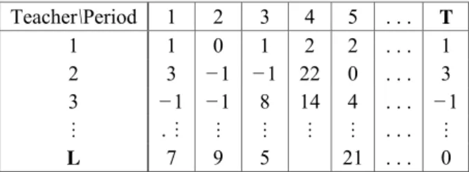
Definition 3. A timetable is a semi feasible solution of type b if it satisfies the restrictions (a) and (c).

In a similar way we represent such a semi feasible solution as a L T× matrix

(Sltb), L=|L|, with values in { 1, 0,1,..., }− J [10]. Entries of the matrix mean subjects for

the teacher l at the time period t if b 0

lt

S > , and free time if b 0

lt

S ≤ . The case b 1

lt

S = −

means that the time period t is unavailable for the teacher l. In Figure 2 we present an example of ( b)

lt

S .

Teacher\Period 1 2 3 4 5 . . . T

1 1 0 1 2 2 . . . 1

2 3 −1 −1 22 0 . . . 3

3 −1 −1 8 14 4 . . . −1

# . # # # # # . . . #

L 7 9 5 21 . . . 0

Figure 2: Semi feasible solution of type b

The advantage of this representation is that it eliminates conflicts for teachers. The occurrence of conflicts in column happens when in a given period t more than one teacher is allocated to a class.

We say that a matrix Sa (a matrix Sb) contains m conflicts if m is a minimal number of its entries which vanishing lead that the restrictions (a) (restrictions (b)) hold. Sure, the restrictions (c) are not satisfied in this case.

Proposition 1. An arbitrary semi feasible solution of type a can be reduced to a semi feasible solution of type b in polynomial time without increasing of the number of conflicts.

Proof: Let m denote the number of conflicts for a solution a

S . We replace m entries in

a

S by 0 in such a way that the restrictions (a) hold and denote the modified matrix by

restriction (c) we identify the lost lessons for each teacher and spread these lessons through 0 entries of the Sb. As a result, the restrictions (c) hold, but the restrictions (b) may be not satisfied. So, the b

S is semi feasible solution of type b. Obviously, the number of conflicts is at most m which complete the proof.

Proposition 2. An arbitrary semi feasible solution of type b can be reduced to a semi feasible solution of type a in polynomial time without increasing of the number of conflicts.

The proof is similar.

It is noticed that an arbitrary feasible solution can be presented as a solution _Sa or Sb, but the inverse statement is not true.

For a semi feasible solution Xlet us introduce the following penalty function:

( ) ( ) lt lta( ) kt ktb( ),

l L t T k K t T

F X F X λ f X µ f X

∈ ∈ ∈ ∈

= +

∑∑

∑ ∑

where min(λ,µ) > max(α, ,) and the functions fa( )X , fb( )X are defined the number of violations of the restrictions (a) and (b) correspondingly. If F X( )=F X( ) then X is a feasible solution. If F X( )=0 then X is optimal solution. But the optimal solution may have a positive value of the penalty function.

4. STARTING SOLUTION

In order to get a starting semi feasible solution for the local search methods we use the well known assignment problem [8]. We apply it for each time period t one by one with adaptation of the problem parameters. As a result we create a semi feasible solution of type b.

Let us introduce auxiliary variables

1, if teacher has a lesson in class in time period , 0, otherwise.

kl

l k t

z =⎧⎨ ⎩

Sure, if the set K l( )={k∈K|∃ ∈j J k j: ( )=k l j, ( )=l} is empty or t∉Tl then we have

to put zkl =0. But if |K l( ) | 1≥ , we have an assignment problem for teachers and classes.

Let b tl( ) denote the total number of lessons which are not included in the starting timetable for teacher l up to the time period t, c tl( ) is the cardinality of the set

\ {1,..., 1}

l

( ) ( ) / ( ), if ( ) ( ), ( ), ,

, if ( ) ( ), ( ), ,

1, if ,

0, otherwise,

l kl l l l l

l l l

t kl

l

b t h t c t b t c t k K l t T

H b t c t k K l t T

H

t T

< ∈ ∈

⎧ ⎪ _{= ∈ ∈} ⎪ =_⎨ − ∉ ⎪ ⎪⎩

where H is large number. Now, the assignment problem for the time period t∈T is the following:

max klt kl

k K l L H z

∈ ∈

∑ ∑

s.t. kl 1, ,

l L

z k K

∈ ≤ ∈

∑

z l L

∈

≤ ∈

∑

{0,1}, , .

kl

z ∈ l∈L k∈K

Let zkl* be the optimal solution of the problem. Define

*

0 *

1, if ,

, if 1, , ( ),

min{ | ( ) 0}, if ( ) ( ), 0 and ,

0 for all other cases.

l

kl l

lt

kl l l k K kl l

t T

k z t T k K l

S

k k h t b t c t _∈ z t T

− ∉ ⎧ ⎪ = ∈ ∈ ⎪ =⎨

= > = = ∈

⎪ ⎪ ⎩

∑

In order to get a semi feasible solution of type b we should define a subject j for each positive entry of the matrix (Slt). By definition of the parameters

t kl

H , the set of appropriated subjects is not empty. We select one of them at random.

5. NEIGHBORHOODS

Now we introduce four families of neighborhoods:

– N Si( a),i≥1, denote swap neighborhoods of a semi feasible solution a

S ,

– ( b), 1

i

N S i≥ , denote swap neighborhoods of a semi feasible solution b

S , – KL Si( a), i>1, denote Kernighan–Lin neighborhoods of

a

S , – KL Si( b),i>1, denote Kernighan–Lin neighborhoods of

b

S . The neighborhood 1( )

a

N S consists of neighboring solutions which are obtained from Sa by swapping two different values of a given row in the matrix (Skta). Each element in this neighborhood is associated with a triplet <k t t, ,′ ′′>, where t′ and t′′ are the time periods, k is the class, and a

kt S ′ and

a kt

S ′′ are the interchanged subjects. For i > 1,

( a) i

triplets {<k t t, ,′ ′′j j>}j i≤, k∈K is fixed. Families ( ) b i

N S are defined in a similar way. Moreover, only non-negative values of the matrix (Sltb) can be interchanged. We note that arbitrary feasible solution can be reached with the use of an appropriate sequence of neighboring solutions for the neighborhoods 1( )

a

N S or 1( ) b N S .

A Kernighan–Lin neighborhood KL Si( a) consists of i elements and can be

described by the following steps [5].

1. Choose a triplet <k t t, ,′ ′′> such that the corresponding neighboring solution

1( )

a

S′ ∈N S is the best even if it is worse than Sa. 2. Put a:

S =S′.

3. Repeat steps 1, 2 i times; if a triplet was used at steps 1 or 2 of previous iterations, it can not be used any more.

The sequence of triplets {<k t t, ,′ ′′j j>}j i≤ defines i neighbors Sj of the solution a

S . We say that a

S is a local minimum with respect to the KLi–neighborhood if

( a) ( j)

F S ≤F S for all j≤i. A local minimum with respect to the KLi– neighborhood

is a local minimum with respect to N1 and is not necessary a local minimum with respect to Ni, i>1. Family ( )

b i

KL S is defined similarly.

Figure 3: Typical PTSR behavior, p = 0.5

6. PROBABILISTIC TABU SEARCH

for short). Let Np denote a random part of the neighborhood N1. Each element of the 1

N is included into the p

N with probability p > 0 independently from other elements. We use this randomized neighborhood on each iteration of the PTSR. If Np= /0 for an iteration of the algorithm we omit it. The tabu list consists of the triplets <k t t, ,′ ′′> or

, , l t t′ ′′

< > according to the solution representations. We change the solution representation for diversification of the search if the best found solution S* is not updated for a long time. The framework of the PTSR is the following:

PTSR Algorithm

1. Compute a starting solution S, put S*:=S and create empty tabu list. 2. Repeat the following sequence until the stopping condition is met:

(a) Find the best nontabu neighbor S′ ∈Np( )S . (b) Put S:=S′, and update the tabu list.

If *

( ) ( )

F S <F S then _S*_:=S.

If F S( )=0 then goto 3.

(c) Change representation of the current solution and put S:=S* if S* is not updated during prescribed number of iterations.

3. Return S*.

Figure 3 shows the typical behavior of the PTSR. By small square we indicate the iterations when the incumbent solution S* is updated. It is easy to identify the iteration 3000 when the solution representation is changed. We return to the best found solution (step 2(c) S:=S*) and get a new type of curve. As a result, new incumbent solutions founded.

7. VARIABLE NEIGHBORHOOD SEARCH

We adjust the framework of the Variable Neighborhood Search (VNS) meta-heuristic [3] for our problem and change not only the neighborhoods but solution representations as well.

VNSR Algorithm

1. Compute a starting solution S and sizes of neighborhood imax, jmax. 2. Repeat the following sequence until the stopping condition is met:

(a) Set i := 1; if F S( )=0 then goto 3. (b) Repeat the following steps until i=imax:

i) Shaking. Generate a solution S′ at random from the N Si( ).

iii) Large neighborhood search. Apply the local descent algorithm with respect to

max

j

KL neighborhood. Denote the obtained local minimum as S′′.

iv) Move or not. If F S( ′′ <) F S( ) then S:=S′′ and go to 2(a); otherwise, set

1

i← +i .

(c) Change the solution representation and go to 2(a). 3. Return S.

Figure 4 shows the typical behavior of the VNSR. The generation of random solution at the step Shaking is shown by dotted lines. One can observe large peaks which correspond to random jumps by i≤imax triplets. The continuous lines show the local descent under the N1 neighborhood. The small dotted lines correspond to the local search

under the KL–neighborhood. Note that the current solution S in this algorithm is actually the incumbent solution. So, additional intensification actions are not required.

8. COMPUTATIONAL RESULTS

The developed software are tested on random benchmarks with real dimensions for the School: K = 44, L = 120, T= × =6 3 18 and J=44 18× =792.

Figure 4: Typical VNSR behavior, imax=5, jmax=30

Each teacher has T/2 available time periods and 20% of them are inconvenient. Each class has T lessons. The penalty coefficients are defined as follows: α = +1 α′,

3

Table 1: Computational results for the first class of benchmarks

PTSR VNS VNSR N

%Opt Aver Worst %Opt Aver Worst %Opt Aver Worst Opt

1 97 92.05 95.0 96 92.04 94.0 93 92.07 93.0 92

2 89 78.16 80.0 81 78.44 83.0 87 78.32 81.0 78

3 100 137.0 137.0 93 137.09 140.0 93 137.11 140.0 137

4 36 97.96 101.0 38 97.9 101.0 52 97.69 103.0 97

5 90 97.16 99.0 83 97.31 100.0 87 97.28 103.0 97

Table 1 shows the optimal values (Opt) for 5 instances and frequency (%Opt) of finding this values by metaheuristics. We solve each instance 100 times and present the average values of the best found solutions (Aver) and the worst values (Worst). Note that the difference between these columns is quite small. So, we have robust local search methods. For all instances we find the optimal solutions by CPLEX software in about 1.5 hours. The metaheuristics discover these solutions in 1.5 min in average. For comparing, we present the result for VNS algorithm without changing representations. For easy instances (all except 4) the both variants VNS and VNSR show the same results. But for the difficult instance 4, where the frequency of finding the optimal solution is small, we observe some advantages of VNSR against VNS. The same effect we can see for another class of test instances. We test the algorithms for benchmarks with the same dimensions but now each teacher has 30% of available time periods and 20% of them are inconvenient for teaching. In other words, the teachers are busier.

Table 2: Computational results for the second class of benchmarks

PTSR VNS VNSR N

%Opt Aver Worst %Opt Aver Worst %Opt Aver Worst Opt

1 18 82.3 86.0 62 80.48 83.0 58 80.54 83 80

2 24 112.38 118 58 110.9 113.0 76 110.56 113.0 110

3 16 139.56 145.0 50 137.7 141.0 40 137.8 140.0 137

4 0 137.16 155.0 0 137.84 153.0 6 132.5 144.0 124

5 28 121.02 125.0 42 121.04 130.0 48 120.58 130.0 119

9. CONCLUSIONS

In this paper we consider the teacher/class timetabling problem and develop local search heuristics based on idea of FSS approach. Two types of solution representations are used in the heuristics and systematically alternate during the search process. We show by computational experiments that idea of two equivalent but not identical solution representations is useful for this timetable problem. We believe that the FSS approach can improve the local search heuristics for other NP-hard problems.

Acknowledgment: This work was partially supported by Russian Foundation of Basic Research, grant 06-01-00075.

REFERENCES

[1] Garey, M.R., and Johnson, D.S., Computers and Intractability: A Guide to the Theory of NP– Completeness, Freeman, San Francisco, CA, 1979.

[2] Glover, F., and Laguna, M., Tabu Search, Kluwer Academic Publishers, Boston–Dordrecht– London, 1997.

[3] Hansen, P., Mladenović, N., "Developments of Variable Neighborhood Search", in: Ribeiro, C.C., Hansen, P. (eds.) Essays and Surveys in Metaheuristics, Kluwer Academic Publishers, 2002, 415-440.

[4] Hertz, A., Plumettaz, M., and Zufferey, N. "Variable space search for graph coloring", GERAD technical report g-2006-81, Montreal 2006 (to appear in Discrete Applied Mathematics).

[5] Kernighan, B.W., and Lin, S., "An efficient heuristic procedure for partitioning graphs", Bell System Technical Journal, 49 (1970) 291-307.

[6] Kochetov, Y., Alekseeva, E., Levanova, T., and Loresh, M., "Large neighborhood local search for the p–median problem", Yugoslav Journal of Operations Research, 15 (1) (2005) 53-63.

[7] Mladenović, N., Plastria, F., and Urošević, D., "Reformulation descent applied to circle packing problems”, Computers and Operations Research, 32 (9) (2005) 2419-2434.

[8] Papadimitriou, C.H., and Steiglitz, K., Combinatorial Optimization: Algorithms and Complexity, Prentice-Hall, Englewood Cliffs, NJ, 1982.

[9] Petrovic, S., and Burke, E., "University timetabling”, in: J.Y-T. Leung (ed.) Handbook of Scheduling: Algorithms, Models, and Performance Analysis, Chapman&Hall/CRC, 2004, 45.1-45.23.