!"#$$ % &'( ( % )
#
* + , - *.,
/ ' 0 1
223"4#5 , - ( ,-( % )
' 6
, -
,-/ ' 0 1
2$53"#5! , - ( ,-( % )
In this work, we introduce an inverse formulation to be applied in the identification of a rheological parameter associated to non-Newtonian fluids. It is built upon a creeping flow through a 4 to 1 axisymmetric abrupt contraction. The fluid is modeled by the Generalized Newtonian Fluid constitutive equation. The viscosity function is based on the one proposed by Souza Mendes et al. (1995). It predicts an extensional elastic behavior, controlled by a rheological parameter θ, which is the parameter determined via the proposed identification procedure. The numerical solution of the forward problem, needed in the iterative procedure introduced by the inverse formulation, is obtained through the finite volume method. A sensitivity analysis is also performed to evaluate the effect of the parameter θ on the dimensionless pressure drop through the contraction. The optimization algorithm is based on an iterative method to find the minimum of the cost function, which is given by the least square difference between numerical and experimental values of the dimensionless pressure drop. The gradient method was used to update the parameter θ, starting from the cost function gradient. The results obtained with the sensitivity analysis validated the adequacy of the proposed cost function, which is a key aspect on the identification formulation. Moreover, it shows that the method provides an attractive alternative for estimation of rheological properties.
Keywords: non-Newtonian fluid, rheological properties, contraction flow, viscoelasticity, inverse analysis, parameters identification
Introduction
1Non-Newtonian fluids are widely used in important industrial
applications, from oil exploitation to food manufacturing, passing through biomedical processes. Therefore, the numerical simulation of processes employing these fluids is a very useful and important tool. However, the non-Newtonian constitutive models are very complex, andusually require a significant amount of experimental data to determine the rheological parameters and, therefore, to calibrate and validate the final model. In the present work, we propose an inverse formulation aiming at estimating rheological properties associated to a nonlinear non-Newtonian fluid model.
Inverse formulations are used to improve a mathematical model of a real system, combining physical principles with experimental data (Banks and Kunish, 1989). The use of such an approach has proven very useful in a wide range of applied fields, from Vibrations (Castello et al., 2008) to Biological systems (Prud’homme and Jasmin, 2006). The main idea is to identify a set of parameters such that, for a desired range of operating conditions, the model outputs matches the actual system outputs, when both are submitted to the same inputs. Due to the lack of available
information and unavoidable measurement errors, system
identification methods can only lead to an approximation of the system’s response.
Important studies regarding optimal conditions and control properties of fluid flows, directly connected to inverse formulations, were developed (Kunish and Marduel, 2000). Different approaches were used to obtain rheological parameters, and this subject still requires lots of attention, especially when complex flows are involved. Within the realm of flow optimization, Fourestey and Moubachir (2005) analyzed the drag reduction of a Newtonian flow through a rotating cylinder, and solved the inverse problem using different algorithms. Kunish and Marduel (2000) used the optimal control formulation and the Phan Thien-Tanner (PTT) model in an abrupt contraction flow to obtain the optimal temperature at the boundary that would give the lowest recirculation zone. Focusing on
Paper accepted November, 2009. Technical Editor: Paulo Eigi Miyagi
estimating rheological parameters, Bernardin and Nouar (1998) used experimental and numerical results of angular torque in a transient Couette flow of an Oldroyd fluid to identify rheological parameters. Sarkar and Gupta (2000) used finite element simulation to obtain results of entrance pressure drop in a contraction flow. Mitsoulis et al. (1998) used the SIMPLEX optimization to improve the value of extensional viscosity parameters, minimizing the difference between the entrance pressure drop predicted numerically, and the ones obtained experimentally with a capillary rheometer. The results showed that the method provides an attractive alternative for estimation of the extensional viscosity. More recently, inverse formulations tailored to non-Newtonian Fluids were developed by Yeow et al. (2005) and by Park et al. (2007 and 2009). Park et al. (2007) employed a method of estimating rheological parameters, using velocity measurements of secondary flows in a square pipe. In a following work, Park et al. (2009) used the same technique in a pulsatile flow through a circular cylinder, and estimated simultaneously five rheological parameters of a differential constitutive equation for viscoelastic fluids. The results obtained were very promising, even when noisy velocity measurements were employed for the parameter identification.
Our inverse formulation builds upon an abrupt 4:1 axisymmetric contraction non-Newtonian flow. The Generalized Newtonian constitutive equation was used, with a viscosity function that takes into account shear and extensional fluid behavior, through a flow classification index and a rheological parameter, namely, θ. The formulation, which can be cast as an optimal control problem, phrases the identification problem as the search for an optimal set of the parameter θ, which minimizes a functional cost relating the experimental and numerical pressure drop through the contraction. A sensitive analysis is performed to evaluate the effectiveness of the pressure drop as the performance index. Moreover, this analysis provides a systematic tool to better understand the complex phenomena involved in the system.
Nomenclature
Cu = Carreau number, dimensionless C = Couette correction
d = Diameter of the capillary tube, m D = Diameter of the upstream tube, m D = rate of strain tensor, s-1
J = cost function
Lent = length of the upstream tube, m Lcap = length of the capillary tube, m Lv = detachment length, m ns = shear power-law index nu = extensional power-law index p = pressure, Pa
R = flow classifier, dimensionless
R' = modified flow classifier, dimensionless
Re = Reynolds number, dimensionless u = axial velocity component, m/s v = radial velocity component, m/s v = velocity vector, W/(m2 K)
We = Weissemberg number, dimensionless W = vorticity vector, s-1
Greek Symbols
∆Pcont = pressure drop through the contraction, Pa γ = rate of strain modulus, s-1
η = fluid viscosity, Pa.s
ηs = shear viscosity, Pa.s ηu = extensional viscosity, Pa.s λs = shear time constant, s λu = extensional time constant, s
θ = rheological parameter, dimensionless ρ = fluid density, kg/m3
Τ = stress tensor, Pa
Flow Modeling: Forward Problem
As mentioned before, the inverse analysis relies upon a mathematical model that describes the nonlinear response of a non-Newtonian fluid, and contains the sought parameters. The resulting mathematical problem, namely the Forward Problem, is usually solved every iteration of an inverse algorithm and, therefore, should be as simple as possible to guarantee the feasibility of the identification process. Here below, the adopted model along with its numerical solution is addressed.
The physical scenario, in which the parameter identification takes place, consists in a contraction flow that mimics the one found in a capillary extrusion rheometer, shown schematically in Fig. 1. The flow geometry leads to the formation of complex recirculation patterns related to the elastic behavior of the fluid and, therefore, prone to provide proper information for the parameters identification. The entrance angle of the capillary tube is taken as 900, in order to increase the pressure drop through the contraction.
The geometry under study is depicted in Fig. 2. The flow is assumed to be laminar, incompressible, steady, and axisymmetric. Moreover, all properties are considered to be temperature-independent.
Taking into consideration the hypothesis above, the mass conservation equation is written as:
divv=0 (1)
where v=ueˆx+veˆr is the velocity vector, and u and v are the velocity components on the axial and radial directions, respectively. The momentum equation is given by:
Figure 1. Scheme of the capillary rheometer.
Figure 2. The geometry.
div ( ) p div
ρ v⊗v = −∇ + τ (2)
where ρ is the density, p is the pressure and τ is the extra-stress tensor, which is related to the flow kinematics by the Generalized Newtonian Liquid constitutive equation (Bird et al., 1987):
2
τ= ηD (3)
In this equation, ≡ ∇ + ∇[ ( ) ] 2T /
D v v is the rate of strain tensor,
and η is the non-Newtonian viscosity function. For simplicity, the only elastic behavior considered here is the extensional (thickening) viscosity, whose contribution is taken into account through the viscosity function given by a weighted average between extensional and shear viscosities:
η = ηs(γ˙ )R
θ
ηu(γ˙ )(1-R
θ)
(4)
This equation was first introduced with θ = 0 in Souza Mendes et al. (1995). The functions ηsand ηu are the shear and extensional
viscosities respectively, and γ˙ =[2tr(D2)]1/2 is the modulus of the strain rate tensor. The quantity R is a flow classifier, taking the value equal to 0 in pure extension and to 1 in shear flows (Thompson et al., 1999). It is defined as:
(
)
( )
2 1
2 2
tr
2
( ) 1
R
R R
tr R
− ′
′ = =
′ +
DW WD
D
(5)
where W=W− Ω is the relative-rate-of-rotation tensor,
[ ( ) ] 2T
= ∇ − ∇ /
to the rate of rotation of D following the motion (Thompson et al.,
1999 and Thompson and Souza Mendes, 2005). θ is a new
rheological parameter, which is proposed here as an attempt to better describe the fluid behavior. The parameter θ defines, along with the flow classifierR, a geometrically weighted average between shear and extensional viscosities. All rheological parameters are supposed to be known a priori, in order to build a suitable model for numerical simulations. Indeed, the motivation of the present work relies on the estimation of those parameters, and a methodology for determining θ is the focus here.
The shear and extensional viscosity functions ηs(γ˙) and ηu(γ˙)
are given by the Carreau equations:
ηs = ηs0 [1+ (λsγ˙ )2]((ns -1)/2) (6)
ηu = ηu0 [1+ (λuγ˙ ) 2
]((nu -1)/2) (7)
where ηs0 and ηu0 are the low strain rate viscosities, λs and λu are the
time constants, ns and nu are the power-law indexes. In order to
simplify the presentation and the assessment of the proposed formulation, these quantities are considered to be previously determined by independent experiments.
Considering the geometry described by Figure 2, the boundary conditions are given by:
• non-slip and impermeability at walls: u = v = 0
• constant inlet velocity: (0 )u ,r =u, v(0,r) = 0 • developed flow at outlet: ∂/∂ =x 0
• symmetry at the centerline (r=0): ∂ /∂ =u r 0, v = 0
The governing dimensionless groups are obtained using the following dimensionless variables1:
2
ˆ ˆ ˆ
u= /u U v= /v U p= /p Uρ (8)
τˆ = τ/ρU2 γ
˙ˆ = γ˙/γ˙c ηˆ = η/ηs0 (9)
In the definitions above, U is the average velocity at the smaller diameter (capillary) tube, γ˙c = 8U(3ns+1)/(4ns d)is the characteristic
strain rate modulus and d is the capillary diameter. The Reynolds number is defined as:
0
s
Ud Re ρ
η
= (10)
The Carreau and Weissenberg numbers are the dimensionless time constants that determine where the transition occurs from the zero-shear-rate plateau to the power-law portion of the shear and extensional viscosity functions. They are respectively defined as:
Cu = λsγ˙c We = λuγ˙c (11)
The Inverse Problem
The present section introduces an inverse problem aiming at the parameter identification associated to the modeling discussed previously. This problem is cast in an optimal control framework, where the vector
Θ
, which contains the sought parameters, plays the role of the control. Indeed, the proposed formulation can be extended to the case where the components of vectorΘ
are functions of the kinematic variables. Roughly speaking, the optimal control problem relates some measured data (like, for instance, the
1 dimensionless quantities are denoted by a hat symbol
ˆ
⋅
, and dimensional variableswithout
pressure drop along the flow) to its model counterpart value. Therefore, the inverse problem consists in finding a minimum of a cost function J p
(
, ,v Θ)
, subjected to constraints provided by the state Eqs. (1), (2) and (3), and by the boundary conditions. This cost function should reflect the mismatch between measured data and modeling output.The appropriate choice of the cost function J plays a crucial role in obtaining the sought parameters, and it is very difficult to have any a priori idea of its optimal form. For instance, Park et al. (2007 and 2009) deals with the identification of rheological parameters by using velocity measurements. The cost function choice should take into consideration the feasibility of the experiments and, at the same time, the good conditioning of the mathematical problem to be solved. Typically, a functional defined as the square of the difference between model and experimental data is taken, leading to a least square constrained problem that might be solved by means of a numerical technique. Indeed, least square formulations are the most often used approach within the realm of inverse problems.
In the present work, the scalar θ (see Eq. (4)) is the sought parameter, and the pressure drop through the contraction is the available data. The cost function J is thus defined as:
(
)
2exp 1 1 ( ) ( ) N i i
J u v p C u v p C
N θ θ =
, , ; =
∑
, , ; − (12)where N stands for the number of measurements and C is a dimensionless pressure drop through the contraction, defined as the Couette correction: cont w cap 2 P C τ , ∆
= (13)
In the equation above, ∆Pcont is the pressure drop through the contraction and
τ
w cap, is the wall shear stress at the developedregion of the small diameter tube. The numerical pressure drop through the contraction is obtained extrapolating the linear pressure drop at the developed regions of the larger and capillary tubes, to the contraction section. In a capillary rheometer, pressure measurements are obtained before the contraction and at the exit of the capillary tube (atmospheric pressure), so that the pressure drop would be also taken using a pressure extrapolation from the capillary tube and the pressure measured before the contraction. It is worth mentioning that this is in fact an approximation of the real pressure drop at the contraction, due to experimental limitations.
The above choice of the cost function reflects two main features of the proposed inverse method. As it is applied to a steady-state flow, no integration over the time span of the analysis is necessary. Indeed, an average produced from similar realizations allows the noise reduction in the experimental data, enhancing the reliability of the formulation. The cost function uses the dimensionless pressure drop, which is a global variable associate to a complex flow. This permits the use of standard experimental procedures. On the other hand, it is not possible to evaluate, by means of simple considerations, the sensitivity of this variable with respect to the parameters to be identified, due to the non-linear relationship between the parameter and the final output. This sensitivity plays a crucial role on the efficiency of the inverse method, and will be addressed later on.
Identification of the Rheological Parameters
typical iteration of a gradient minimization method is presented below:
1
( ) ( 1 )
k k k
TJ k n
θ + θ α ′θ
= − = ,..., (14)
where αT is the step length of the algorithm and J’ stands for the
gradient of the cost function J (Eq. 12). The most delicate aspect of the proposed algorithm is the computation of this gradient. A direct computation would lead to a very troublesome numerical problem involving the sensitivities of the state fields with respect to the sought parameters. Here, this computational procedure is replaced by a scheme based on finite difference approximation of the derivative, which is often used in similar problems (Gunzburger, 2003):
( ) ( )
0 2
J J
J θ θ θ θ θ
θ
′ + ∆ − − ∆
≈ ∆ →
∆
(15)
The computational algorithm is summarized as: Step 0 - Set k = 0 and choose the initial guess θ0
Step 1 - Solve the forward problem and obtain the estimated values for Ck
Step 2 - Compute (J θk)(Eq. 12) and its gradient J′(θk)using
Eq. (15)
Step 3 - Choose a descent step αT
Step 4 - Update the sought parameters by using
1 ( )
k k TJ k
θ θ α ′θ
+ = −
Step 5 - Check convergence. If yes, end. If no, go to step 1. The
convergence was considered satisfactory if| J |≤10−5, since the sought parameter θ0 remains unaffected for
values of tolerance below 10-5.
To obtain a solution for the Forward Problem (Step 1), the mass and momentum conservation equations (Eqs. (1) and (2)), together with the constitutive equation described before (Eq. (3)), were discretized by the Finite Volume Method (Patankar, 1980). Staggered velocity components were employed to avoid unrealistic pressure fields. The pressure-velocity coupling was handled by the SIMPLEC algorithm (Van Doormaal and Raithby, 1984). The resulting algebraic system was solved by the TDMA line-by-line algorithm, coupled with the block correction algorithm (Settari and Aziz, 1973) to increase the convergence rate. The solution was considered converged, when the normalized residue of the conservation equations was less than 10-5. It is worth mentioning that no significant changes on the velocity and pressure fields were observed for lower values of tolerance. Moreover, the step length was taking constant and equal to 1 along all numerical experiments.
In order to investigate the above numerical approach within the conditions engendered by the inverse formulation, a convergence study was carried out. A non-uniform mesh with 280 control volumes in the axial direction and 110 control volumes in the radial direction was used. The mesh was refined near the contraction and near the walls. Some tests were performed to validate the numerical solution. The results for the Couette correction and for the dimensionless detachment length (Lv/D) for a Newtonian fluid were compared to the
ones obtained in the literature. Errors equal to 0.8 % for the Couette correction, and to 4.7 % for the detachment length were found. The velocity profiles were obtained for three different meshes, for Newtonian and non-Newtonian fluids (ns=1,nu=2,θ=1). The
differences between the chosen mesh and a more refined mesh (with 360 control volumes in axial direction and 130 control volumes in radial direction) were below 1%.
Numerical Results
The effectiveness of the proposed formulation is assessed through the axisymmetric abrupt contraction flow, depicted in Fig. 2. This first evaluation of the proposed method uses only synthetic data produced by numerical simulations of the Forward Problem. The motivation for using this geometry is twofold: the reproduction of experimental likely scenarios and the presence of extensional and shear deformation modes along the flow. The geometric parameters are Lent/D = Lcap/D = 2, and D/d = 4. All the situations analyzed
here were obtained for low Reynolds numbers ( 3
10
Re≤ −), in order to avoid inertia effects.
The sensitivity of the measured data with respect to the sought parameters is one of the main issues when developing an inverse method aiming at parameter identification. Here, a sensitivity analysis is performed by analyzing the effect of the rheological parameters on the flow pattern. Particular emphasis is placed on the elastic characteristics of the fluid response and, also, on the role played by the parameter θ.
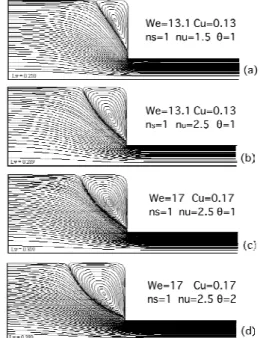
Figures 3 and 4 show the streamlines, the flow classifier (Eq. 5) and the viscosity fields for different set of rheological parameters, in order to evaluate their effects on the flow pattern. These results were obtained for Boger fluids, i.e., constant shear viscosity, ns = 1. It can
be observed the presence of the corner vortex, and how it increases by stimulating the fluid elasticity (increasing We, nu ,θ). Analyzing
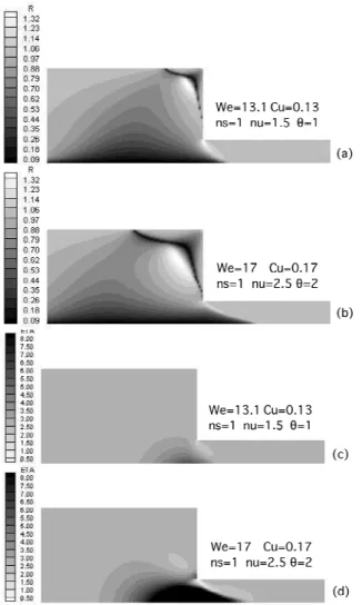
the flow classifier field (Figs. 4(a) and 4(b)), it is noted that shear flow (R = 1) occurs close to the walls, and also everywhere away from the contraction plane. Extensional flow (R = 0, dark region) occurs in a large region located just upstream the contraction plane, and a nearly rigid body motion (R > 1, light region) occurs in the corner vortex. The viscosity fields show a smooth viscosity variation near the contraction region. Away from the contraction, the viscosity is constant and equal to the shear viscosity, since there is no extension. As the fluid approaches the centerline, close to the contraction zone, flow is predominantly extensional, and largest values of viscosity are obtained.
Figure 3. Streamlines for different rheological parameters.
The effect of We and nu on the vortex size and Couette
already mentioned, the vortex size increases with fluid elasticity. This result is in accordance with the literature (Boger et al., 1986; Boger et al., 1992; Boger and Binnington, 1994), and stresses the importance of the extensional behavior on flow pattern. The pressure drop through the contraction also increases monotonically with the Weissenberg number and with the exponent nu. It is worth
mentioning that for a Newtonian fluid, the Couette correction is equal to 0.58.
Figure 4. (a) and (b): Flow classifier field; (c) and (d): viscosity field. Results for different rheological parameters.
Figure 5. Vortex size versus We for ns = 1, θθθθ = 1 and nu = 1.5, 2 and 2.
Figure 6. Couette Correction versus We for ns = 0.5, 0.75 and 1, θθθθ = 1 and nu = 1.5, 2 and 2.
From now on, some results directly related to the parameter identification problem will be presented. The proposed formulation is expected to handle the identification of several different parameters simultaneously. Despite that, here only the new rheological parameter θ is assumed to be unknown. This allows a deeper understanding of the role played by θ, by means of a sensitivity analysis (Guzbunger, 2003). Further, it leads to a simpler numerical problem, which is suitable for assessing and testing the proposed formulation. Fig. 7 presents a sensitivity analysis of the Couette correction with the sought parameter θ. The Couette correction was normalized with the value obtained with θ = 1. It can be observed that the Couette correction can be quite sensitive to the parameter θ, leading to the conclusion that it is a reasonable choice for the variable to be used on the identification procedure. However, it’s worth mentioning that the choice of the Couette correction replacing the dimensional pressure drop adds an uncertainty associated to the wall shear stress, which also needs to be measured experimentally. The impact of this uncertainty on the identification procedure will be assessed later on.
Figure 7. Normalized Couette Correction versus θθθθ for ns = 1, We = 13.1 and nu = 1.5, 2 and 2.
Figures 8 to 10 show the normalized cost function (J∗ J J(θ 1)
= / = )
technique, as described in the previous section. Moreover, the inverse analysis employs a coarser grid than the one used to obtain the synthetic data in order to avoid the so called inverse crime. The results show that the cost function behavior is strongly dependent on the fluid properties and this type of analysis should be used as guide for setting up the experimental conditions. The existence of local minima is a drawback for the identification procedure and, therefore, should be avoided. Figures 8 and 9 show that at the range of θ analyzed, some local minima tend to appear, as the fluid extensional behavior is more pronounced (higher nu). However, the
shear thinning fluid behavior (ns < 1) is favorable to the
identification procedure, since it seems to delay the appearance of a local minimum. Figure 10 shows the effect of Weon the cost function. Once again, it is noted that the increase of elastic effects due to extension (higher We) leads to the disappearance of a local minimum (see case with nu = 2) within the analyzed range.
Figure 8. Normalized cost function versus θθθθ for ns = 1 and different values of nu.
Figure 9. Normalized cost function versus θθθθ for ns = 0.5 and different values of nu.
Figure 10. Normalized cost function versus θθθθ. Effect of We.
Any inverse formulation is subject to two major error sources, namely: measurement noise and uncertainties in the modeling (e.g. boundary conditions, driven forces, etc.). The former is not considered a significant source error for the present situation as long as data is only taken from a steady-state flow, and noise can be reduced by averaging the data. On the other hand, the use of the normalized pressure drop represented by the Couette correction constitutes an additional uncertainty source for the inverse analysis. Its impacts on the estimated value of θ are investigated through a simple strategy: different values of the experimental Couette correction replace the actual one. They are chosen such that the deviation from the correct value reaches 2%, more specifically the value used is given by
exp
(1−δ)C , with − .0 02≤δ≤ .0 02. Figure 11
depicts the variation of the cost minima with regard to the level of uncertainty. Roughly speaking, a deviation of 2% leads to a final error in the parameter identification of almost 5%.
Figure 11. Normalized cost function versus θθθθ. Effect of the uncertainty δδδδ on Couette correction values.
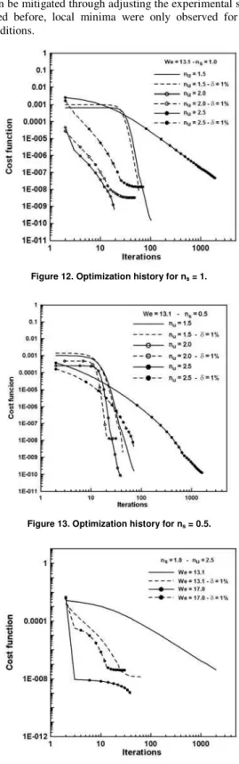
Finally, the conditions for convergence of the iterative process are investigated. Figures 12 to 14 show the number of iterations needed to obtain the parameter θ for different flow conditions. It can
initial guess for θ plays an important role and can lead to errors in
the parameter identification, since the value obtained for θ can converge for a local minimum. This behavior suggests that additional regularization techniques may be necessary to improve the identification procedure. Besides, as the proposed methodology was designed respecting a balance between experimental and numerical feasibilities, this inconvenient dependence on the initial guess can be mitigated through adjusting the experimental setup. As mentioned before, local minima were only observed for specific flow conditions.
Figure 12. Optimization history for ns = 1.
Figure 13. Optimization history for ns = 0.5.
Figure 14. Optimization history for ns = 1 and nu = 2.5.
Final Remarks
The determination of rheological parameters using data obtained through standard viscometric flows opens the possibility of building reliable numerical models, which can be used in the design of complex engineered systems. As long as those experiments are very well established, the main challenge becomes the way experimental data can be explored to be integrated with the numerical model. This can be systematically carried out by inverse formulations.
The present work introduces an inverse formulation aiming at the identification of rheological parameters associated to a nonlinear constitutive equation. Although the formulation has a potential to deal with different parameters, only the determination of θ has been assessed. An extensive sensitivity analysis is performed. The results obtained confirm the adequacy of the proposed cost function involving the pressure drop along the flow, which is a key aspect on the identification formulation. Moreover, an uncertainty analysis is also carried out, investigating the reliability of the inverse formulation, which has proven efficient and useful for more generic constitutive equations. The results for the identification procedure showed that convergence is obtained fast, but the initial guess is important, since some local minima can appear. Testing this formulation with real data, and also identifying other rheological parameters are subjects under study. Uncertainties should be specified for experimental and numerical results.
Acknowledgements
Financial support for the present research was provided by CAPES and CNPq.
References
Banks, H.T. and Kunisch, K., 1989, “Estimation Techniques for Distributed Parameter Systems”, Birkhauser – Systems & Control: Foundations & Applications. Boston.
Bernardin, D. and Nouar, C., 1998, “Transient Couette flows of Oldroyd’s fluids under imposed torques”, Journal of Non-Newtonian Fluid Mechanics, Vol. 77, pp. 201-211.
Boger, D.V., Hur, D.U., Binnington, R.J., 1986, “Further observations of elastic effects in tubular entry flows”, Journal of Non-Newtonian Fluid Mechanics, Vol. 20, pp. 31-49.
Boger, D.V., Crochet, M.J., Keiller, R.A., 1992, “On viscoelastic flows through abrupt contractions”, Journal of Non-Newtonian Fluid Mechanics, Vol. 44, pp. 267-279.
Boger, D. V., Binnington, R. J., 1994, “Experimental removal of the re-entrant corner singularity in tubular entry flows”, Journal of Rheology,Vol. 38, pp. 300-349.
Castello, D.A., Rochinha, F.A., Roitman, N. and Magluta, C., 2008, “Constitutive parameter estimation of a viscoelastic model with internal variables”, Mechanical Systems and Signal Processing, Vol. 22, pp. 1840-1857.
Fourestey, G., Moubachir, M., 2005, “Solving inverse problems involving the Navier&Stokes equations discretized by a Lagrange-Galerkin method”, Computer Methods in Applied Mechanics and Engineering, Vol. 194, pp. 877-906.
Gavrus, A., Massoni, E., Chenot, J.L., 1996, “An inverse analysis using a finite element model for identification of rheological parameters”, Journal of Materials Processing Technology, Vol. 60, pp. 447-454.
Gunzburger, M.D., 2003, “Perspectives in Flow Control and Optimization”, Advances in Design and Control, SIAM Society for Industrial Mathematics.
Knabner, P. and Angermann, L., 2003, “Numerical Methods for Elliptic and Parabolic Partial Differential Equations”, 1st Ed., Ed. Springer, New York.
Kunisch, K. and Marduel, X., 2000, “Optimal control of non-isothermal viscoelastic fluid flow”, Journal of Non-Newtoinan Fluid Mechanics, Vol. 88, pp. 261-301.
Nascimento, S.C.C., 2007, “Uma Formulação de Otimização para Identificação de Parâmetros Reológicos de Fluidos Viscoelásticos”, D.Sc. Thesis, Department of Mechanical Engineering, COPPE/UFRJ.
Park, H.M., Hong, S.M. and Lim, J.Y. , 2007, “Estimation of rheological parameters using velocity measurements”, Chemical Engineering Science, Vol. 62, pp. 6806-6815.
Park, H.M., Shin, K.S. and Choi, Y.J., 2009, “Rheometry using velocity measurements”, Rheologica Acta, Vol. 48, pp. 433-445.
Patankar, S.V., 1980, “Numerical Heat Transfer and Fluid Flow”, Hemisphere Publishing Corporation.
Prud’homme, M. and Jasmin, S., 2006, “Inverse solution for a biochemical heat source in a porous medium in the presence of natural convection”, Chemical Engineering Science, Vol. 61, pp. 1667-1675.
Settari, A. and Aziz, K., 1973, “A generalization of the additive correction methods for the iterative solution of matrix equations”, SIAM J. Num. Anal., Vol. 10, pp. 506-521.
Sarkar, D. and Gupta, M., 2000, “Estimation of elongational viscosity using entrance flow simulation”. In: CAE and Related Innovations for Polymer Processing, ASME, MD, Vol. 90, pp. 309-318.
Thompson, R.L, Souza Mendes, P.R. and Naccache, M.F., 1999, “A new constitutive equation and its performance in contraction flows”, Journal of Non-Newtonian Fluid Mechanics, Vol. 86, pp.375-388.
Thompson, R.L, and Souza Mendes, P.R., 2005, “Persistence of straining and flow classification”, Int. Journal of Engineering Science, Vol. 43, pp.79-105.
Van Doormaal, J.P. and Raithby, G.D., 1984, “Enhancements of the SIMPLE Method for Prediction Incompressible Fluid Flows”, Num. Heat Transfer, Vol. 7, pp. 147-163.
Souza Mendes, P.R., Padmanabhan, M., Scriven, L.E. and Macosko, C.W., 1995, “Inelastic constitutive equations for complex flows”, Rheologica Acta, Vol. 34, pp. 209-214.