CERNE
Historic:
Received 07/03/2018 Accepted 23/08/2018
Keywords: Operational research Artifi cial intelligence Forest management
1 Federal University of Minas Gerais, Montes Claros, Minas Gerais, Brazil 2 State University of Montes Claros, Montes Claros Minas Gerais, Brazil 3 University of London, Guildford, United Kingdom
4 Federal University of Recôncavo da Bahia, Cruz das Almas, Bahia, Brazil 5 Federal University of Viçosa, Viçosa, Minas Gerais, Brazil
+Correspondence: araujocaj@gmail.com
DOI: 10.1590/01047760201824032538
Carlos Alberto Araújo Júnior1+, João Batista Mendes2, Adriana Leandra de Assis1, Christian
Dias Cabacinha1, Jonathan James Stocks3, Liniker Fernandes da Silva4, Helio Garcia Leite5
TUNING OF THE METAHEURISTIC VARIABLE NEIGHBORHOOD SEARCH FOR A FOREST PLANNING PROBLEM
ARAÚJO JÚNIOR, C. A.; MENDES, J. B.; ASSIS, A. L.; CABACINHA, C. D.; STOCKS, J. J.; SILVA, L. F. LEITE, H. G.Tuning of the metaheuristic variable neighborhood search for a forest planning problem. CERNE, v. 24,
n. 3, p. 259-268, 2018.
HIGHLIGHTS
VNS is effi cient to solve a forest planning problem.
Algorithm parameters are important to fi nd a good solution quickly.
ABSTRACT
In forest science it is important evaluate new technologies from computational science. This work aimed to test a different kind of metaheuristic called Variable Neighborhood Search in a forest planning problem. The management total area has 4.210 ha distributed in 120 stands in ages between 1 and 6 years old and site index since 22 m to 31 m. The problem was modelled considering the maximization of the net present value subject to the restrictions: annual cut volume between 140.000 m³ and 160.000 m³, harvester ages equal to 5, 6 or 7 years, and the impossibility of division of the management unity at harvester time. It was evaluated different settings for the Variable Neighborhood Search, varying the quantity of neighbours, the neighbourhood structure and number or generations. 30 repetitions were performed for each setting. The results were compared to the one obtained from integer linear programming and linear programming. The integer linear programming considered the best solution obtained after 1 hour of processing. The best setting to the Variable Neighborhood Search was 100 neighbours, a neighbourhood structure with changes in 1%, 2%, 3% and 4% of prescriptions and 500 iterations. The results shown by the Variable Neighborhood Search was 2,77% worse than one obtained by the integer linear programming with 1 hours of processing, and 2,84% worse than the linear programming. It is possible to conclude that the presented metaheuristic can be used satisfactorily in a resolution of forest scheduling problem when the best parameters are chosen.
INTRODUCTION
Forest planning problems can be considered as complex in function of the amount of decision variables, imposed constraints and difficult to obtain all necessary information to develop work plans, mainly because of intrinsic characteristics of forest activities. In this sense, the effective courses-of-actions determination that maximize the enterprise economic returns or that optimize ecological and social aspects, as mentioned by Kaya et al. (2016), Ezquerro et al. (2016), Dong et al. (2016) and Shan et al. (2009), has been done with use of mathematical programming, like Linear Programming (LP), Integer Linear Programming (IP) and Mixed Integer Linear Programming (MIP) for instance (Troncoso et al., 2016).
Although their wide application, these tools had been replaced by more flexible techniques, mainly when there are more impeditive constraints in the models, like constraints of adjacency and singularity, or when nonlinear aspects are taking in account. It occurs because, with these considerations, the problem complexity is augmented and this can avoid a quick convergence to an optimal global solution in a feasible time when we use exact algorithms like branch-and-bound (B&B).
In these cases, when the problems became as belong to NP class (nondeterministic polynomial time), algorithms that can find a good feasible solution and that cannot require the full compliance with some assumption of classical mathematical programming, like additivity and proportionality (Jin et al., 2016), are indicated. This suggests the development and application of heuristics methods (Yoshimoto et al., 2016; Jin et al., 2016; Shan et al., 2009).
A heuristic is an iterative method that employs logic and rules that guide the search of feasible good solutions to a problem, near to optimal solutions but without ensuring the optimality (Kaya et al., 2016; Hillier and Lieberman, 2013; Jin et al., 2016; Ezquerro et al., 2016). Its application for combinatorial problems has been growing in the last years and already pass the number of scientific publications that consider the development and application of exact algorithms (Ezquerro et al., 2016). This occurs because sometimes the acceptance of a too much good solution obtained in a short time can be more interesting than the optimal solution obtained from a process with high computational efforts and time processing.
Heuristics and metaheuristics have been used in forest sector since 1980 (Jin et al., 2016; Ezquerro et al., 2016). Specifically, in forest management their applications have been highlighted as computational resources have been developed. It allows that new works could be done using these methods, mainly in bigger and complex management plans (Dong et al., 2016). In
terms of forest production planning, Kangas et al. (2008) mentioned that the integer nature of forest planning problems and the use of spatial criteriums are important reasons by the increase of popularity of metaheuristics in these problems.
Among the vast number of already developed metaheuristics it is possible to highlight (Boussaid et al., 2013): Tabu Search (TS), Simulated Annealing (SA), Genetic Algorithm (GA), Ant Colony (AC), GRASP and HERO, Particle Swarm Optimization (PSO), Bee Colony (BC), Multi-Agent Systems (MAS) and Artificial Neural Networks (ANN). SA is the most cited methodology (Ezquerro et al., 2016), but considering the advances in studies about artificial intelligence, new metaheuristics arise and it become possible their evaluation in a wide of operation research applications.
Thus, algorithms relatively simple, as local search ones, had been widely used. However, in too many cases it is interesting that these algorithms can be modified or adapted to a specific problem in order to improve their performance. Among these algorithms, the Variable Neighborhood Search (VNS) has been highlighted by its simplicity, efficiency, and robustness in a wide of NP-Hard problems (Doerner et al., 2007). Its basic idea is to change the neighborhood structure to search a better solution for the problem (Affi et al., 2017; Doerner et al., 2007; Glover and Kochenberger, 2003).
There are some works already published about VNS as Affi et al. (2017) for vehicle routing problem, Amous et al. (2017) for capacitated vehicle routing problem, and Brimberg et al. (2017) for capacitated grouping problem, for instance. Despite that, this algorithm was not evaluated on forest production planning problem. In that case, it is important that studies be done in order to evaluate different set of algorithm’s parameters for specific kind of problem, as suggested by Jin et al. (2016) and Shan et al. (2009), since the heuristic performance is highly dependent on the parameters used (Dong et al., 2016) and of the problem considered.
Thus, we evaluated the behavior of VNS metaheuristic in function of variations in parameters values and its relative efficiency comparing with Linear Programming and Integer Linear Programming in solving a forest planning problem.
MATERIAL AND METHODS
Data
and 6 years-old: 339 ha with 1-year-old; 768 ha with 2-year-old; 1,031 ha with 3-year-old; 601 ha with 4-year-old; 958 ha with 5-year-4-year-old; and 513 ha with 6-year-old. Wood production estimates for each stand in each age was obtained from the equation (1), where Vi is the volume for the stand i, Ii is the age of stand i, and Si is the site index for the stand i. It was developed by the authors considering data from a continuous forest inventory. Values of site index ranged from 22 to 31 m considering an index age equals to six-year-old.
Constraint (3) guarantees that all stand areas receives a determinate prescription. Constraints (4) and (5) limit the annual cutting volume between the minimum and maximum demand. Constraint (6), that is considered only in IP model, imposes a unique management alternative for each stand along the horizon plan.
[1]
Prescriptions for each stand considered harvester in one of three ages 5, 6 and 7-year-old, an immediately planting activity after the cut and a time horizon of the forest plan equals to sixteen years. It resulted in 81 management prescription for each stand totaling 9,720 decision variables for each model. Mathematical formulations for the optimization models were based on Model I mentioned by Jonhson and Scheurman (1977) in order to preserve the physical identity of management unit along the horizon plan. The objective was to maximize the net present value under constraints of annual demand between 140,000 m3 and 160,000 m³.
The annual discount rate used was equals to 8 percent, the price of wood sales equals to R$ 80.00 per cubic meter and harvester cost equals to R$ 30.00 per cubic meter. Silvicultural costs ranged according to the age of each stand and were obtained from Binoti (2010): R$ 4,059.05 ha-1 on first-year; R$ 1,627.81 ha-1 on second-year; R$ 757.95 ha-1 on third-year; e R$ 88.12 ha-1 since on fourth-year of forest growth.
Linear and Linear Integer Programming
LP and IP models were formulated as suggest by Rodrigues et al. (2004). A unique difference between ones is the absence of constraint 6 for the LP model, where: GNPV is the global net present value for all the forest (2), in reais; Cij is NPV for stand i when assigned the prescription j, in reais; Xij is the decision variable and represents the proportion area of stand i that will be managed with prescription j; M is the total number of stands; N is the total number of different prescriptions for each stand; Vij(k) is the total volume of wood for the stand i, when assigned the prescription j, in the period k of planning horizon; Dmink and Dmaxk are minimum and maximum wood demand for the period k of the planning horizon.
[2]
[3]
Vij k Xij D k
j N i M (( )( )) ( ) ( ) ( ) min ≥ = =
∑
∑
1 1 [4] [5] [6]The LP and IP models were solved in CPLEX software version 12.7.1 (IBM Corporation, 2017) considering simplex and branch-and-bound algorithms, respectively. It was done on a computer with Windows 10, 64 bits, processor Intel Core i7 with 2.0 GHz and 8Gb of RAM memory. The LP model was used to test if the optimal solution was an integer solution. If this was true, neither IP nor metaheuristic solutions were necessary for our problem.
Variable Neighborhood Search
VNS is an algorithm based on a local search with different neighborhood structures (Doerner et al., 2007). They define a set of modifications that can be applied to a solution in order to create new solutions (Meignan et al., 2012). According to Mladenovic and Hansen (1997), the basic algorithm can be described as a set of steps that starts by the definition about the amount and types of neighborhood structures that will be considered. Then a random solution is obtained (Figure 1). With that, for each iteration and neighborhood structure, the algorithm executes a local search procedure in order to find a solution better than the considered before. If the algorithm does not find no better solution after n iterations, or after evaluates all neighbors, the structure is changed and the local search is done again. This process repeats until all considered neighborhood structures are used. The algorithm finishes when a stop criterium is reached, like as a number of iterations or time of processing.
(i=1) M (j=1) N (ij) X =1
åå
Vij k Xij D k
This study considered a proposed VNS version with four neighborhood structures evaluated in two sets. This way, considering set 1 of neighborhood structure (S1) and the fi rst local search procedure (LS1), 1% of stands from one solution, randomly chosen, had its prescription modifi ed. Local search procedures LS2, LS3, and LS4 considered modifi cations in 2%, 3% and 4% of stands. Set 2 of neighborhood structure (S2) considered local search procedures that execute modifi cations in 10%, 20%, 30% and 40% of stands at a solution. Each stand modifi cation means to change a stand prescription (adopted for all plan horizon) that are chosen randomly for other prescription, also chosen in a random way.
The VNS algorithm evaluated all individuals from a defi ned neighborhood size in each local search procedure. Thus, to identify the infl uence of the number of neighbors, it was tested different sizes for the neighborhoods. It was considered neighborhoods with 1, 10, 30, 50 and 100 neighbors.
It was considered 30 repetitions and different stop criterium (20, 50, 100, 300 and 500 iterations) in each evaluation (arrangement of a set of neighborhood structure and a number of neighbors). The results were evaluated using the Kruskal-Wallis test (K-W) with 5% of probability. Confi guration with best values for average and maximum fi tness, as a loss value for standard deviation at end of processing, was chosen.
Constraints imposed on LP and IP models also were considered for VNS model. In that case, it was considered a penalty for the objective function in function of every broken constraint. Thus, for each volumetric demand constraint that was broken, objective function was decreased in R$ 100.00 per cubic meter in excess or lack at end of each period in the planning horizon. This method is the same adopted by Rodrigues et al. (2004).
Metaheuristic processing was done using MeP (Metaheuristics for Forest Planning) software. It was developed at Operation Research and Forest Modelling Laboratory at the Federal University of Minas Gerais in java language programming.
RESULTS
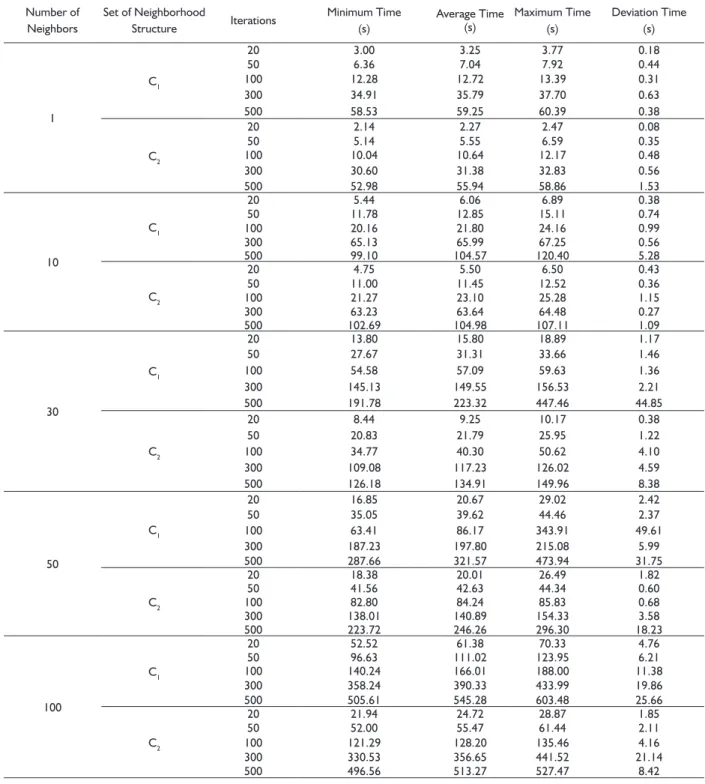
The VNS has its processing interrupted after reach the stop criterium and the processing time ranged according to the parameters values used (Table 1). The smaller processing time was obtained for the confi guration with 1 neighbor, set 2 of neighborhood structure and 20 iterations. The bigger processing time was obtained for 100 neighbors, set 1 of neighborhood structure and 500 iterations.
The parametrization that reached the best results considered a neighborhood with 100 neighbors, set 1 of neighborhood structure and 500 iterations (Table 2). The best solution was 231% superior to the worse solution found (which presented 1 neighbor, set 1 of neighborhood and 20 iterations). In relation to the average and maximum values for fi tness, the worse result was presented for the parametrization with 1 neighbor, set 2 of neighborhood structure and 20 iterations.
The increase in the number of iterations provided improvements on obtained results for all cases analyzed. However, there were not signifi cative differences (p<0.05) between the results obtained for 300 or 500 iterations according to the K-W test. The same occurred when the number of neighbors was increased and, in this case, there weren’t differences between the results found with 50 or 100 neighbors considering the same test (p<0.05). Considering the different sets of neighborhood structure, the increase in the number of solution modifi cations in order to create a new neighbor
TABLE 1 Processing time obtained from evaluations considering different parameters of VNS.
Number of Neighbors
Set of Neighborhood
Structure Iterations
Minimum Time (s)
Average Time (s)
Maximum Time (s)
Deviation Time (s)
1
C1
20 3.00 3.25 3.77 0.18
50 6.36 7.04 7.92 0.44
100 12.28 12.72 13.39 0.31
300 34.91 35.79 37.70 0.63
500 58.53 59.25 60.39 0.38
C2
20 2.14 2.27 2.47 0.08
50 5.14 5.55 6.59 0.35
100 10.04 10.64 12.17 0.48
300 30.60 31.38 32.83 0.56
500 52.98 55.94 58.86 1.53
10
C1
20 5.44 6.06 6.89 0.38
50 11.78 12.85 15.11 0.74
100 20.16 21.80 24.16 0.99
300 65.13 65.99 67.25 0.56
500 99.10 104.57 120.40 5.28
C2
20 4.75 5.50 6.50 0.43
50 11.00 11.45 12.52 0.36
100 21.27 23.10 25.28 1.15
300 63.23 63.64 64.48 0.27
500 102.69 104.98 107.11 1.09
30
C1
20 13.80 15.80 18.89 1.17
50 27.67 31.31 33.66 1.46
100 54.58 57.09 59.63 1.36
300 145.13 149.55 156.53 2.21
500 191.78 223.32 447.46 44.85
C2
20 8.44 9.25 10.17 0.38
50 20.83 21.79 25.95 1.22
100 34.77 40.30 50.62 4.10
300 109.08 117.23 126.02 4.59
500 126.18 134.91 149.96 8.38
50
C1
20 16.85 20.67 29.02 2.42
50 35.05 39.62 44.46 2.37
100 63.41 86.17 343.91 49.61
300 187.23 197.80 215.08 5.99
500 287.66 321.57 473.94 31.75
C2
20 18.38 20.01 26.49 1.82
50 41.56 42.63 44.34 0.60
100 82.80 84.24 85.83 0.68
300 138.01 140.89 154.33 3.58
500 223.72 246.26 296.30 18.23
100
C1
20 52.52 61.38 70.33 4.76
50 96.63 111.02 123.95 6.21
100 140.24 166.01 188.00 11.38
300 358.24 390.33 433.99 19.86
500 505.61 545.28 603.48 25.66
C2
20 21.94 24.72 28.87 1.85
50 52.00 55.47 61.44 2.11
100 121.29 128.20 135.46 4.16
300 330.53 356.65 441.52 21.14
500 496.56 513.27 527.47 8.42
made the results worse and statistically different between the two sets according to the K-W test (p<0.05).
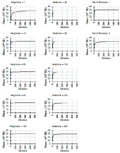
The finding of all test observed that increasing the number of neighbors made the algorithm faster in converge to the best solution with a less number of iterations (Figure 2). The change in the neighborhood structure from type 1 to type 2 decreased the algorithm performance, and it was necessary more iterations in order to reach same results.
The IP model solution was obtained after 1 hour of processing without the algorithm had converged to the global optimal solution. The solution found by the LP model was the global optimal (Table 3). The method that found the best solution was LP followed by the solution obtained by IP model. The best VNS solution was approximately 2.77% inferior to the IP value.
(0.26%). They were divided into 12 from 120 stands and one stand received three different management prescriptions and the other received two prescriptions.
For all methods, the annual harvested volume constraint was reached at best solution found. The period with more or less wood volume production ranged among the methods (Figure 3). Also, there were differences in the total volume produced and
TABLE 2 Processing time obtained from evaluations considering different parameters of VNS.
Number of Neighbors
Set of Neighborhood
Structure Iterations
Minimum Time
(R$)
Average Time (R$)
Maximum Time (R$)
Deviation Time (R$)
1
C1
20 -13,530,547 21,844,848 29,966,401 9,545,235 50 25,612,348 29,301,773 30,300,314 1,042,549 100 29,731,043 30,081,475 30,411,167 181,309 300 29,936,976 30,265,601 30,456,298 137,348 500 30,203,232 30,372,621 30,589,252 112,384
C2
20 -11,626,475 4,169,321 20,560,345 8,787,173 50 6,505,206 15,158,154 27,354,774 5,117,997 100 9,390,474 19,583,982 26,141,177 4,351,402 300 16,363,288 23,162,209 27,682,639 2,432,716 500 21,057,602 26,169,244 29,992,760 1,875,369
10
C1
20 29,967,518 30,221,822 30,510,139 131,327 50 30,060,371 30,342,201 30,636,604 145,786 100 30,184,859 30,460,931 30,692,985 122,702 300 30,413,801 30,632,924 30,872,609 124,340 500 30,468,749 30,696,456 30,933,782 121,521
C2
20 18,617,328 23,361,948 29,735,080 2,819,559 50 21,217,395 25,874,762 29,921,567 2,251,521 100 23,715,073 27,226,132 29,895,782 1,499,920 300 26,561,655 28,812,762 30,151,917 953,241 500 27,050,693 29,471,710 30,244,190 781,815
30
C1
20 30,057,139 30,371,824 30,647,249 128,889 50 30,138,694 30,521,917 30,749,268 134,688 100 30,341,603 30,598,422 30,873,988 126,254 300 30,648,549 30,862,520 31,072,842 112,703 500 30,513,361 30,926,001 31,120,320 143,097
C2
20 20,202,816 26,465,485 29,730,038 2,399,578 50 25,284,828 28,042,636 30,208,252 1,406,012 100 26,882,822 29,323,436 30,271,609 818,677 300 28,530,423 29,677,463 30,231,076 392,551 500 28,760,078 29,811,738 30,186,482 335,134
50
C1
20 30,130,643 30,474,072 30,705,788 133,835 50 30,214,490 30,603,608 30,848,142 123,486 100 30,497,950 30,799,918 31,055,639 121,480 300 30,744,304 30,954,825 31,191,456 104,738 500 30,833,913 31,029,240 31,230,218 104,722
C2
20 24,676,505 27,817,077 30,079,036 1,522,640 50 25,920,450 28,956,130 30,071,751 1,021,629 100 27,277,290 29,509,222 30,255,828 737,163 300 28,553,614 29,776,552 30,268,491 422,628 500 29,569,576 29,989,853 30,249,780 149,766
100
C1
20 30,459,223 30,692,357 30,953,820 132,670 50 30,482,402 30,759,695 31,127,963 161,043 100 30,690,880 30,906,917 31,189,477 122,775 300 30,765,250 31,035,434 31,174,404 95,035 500 30,903,026 31,138,612 31,276,858 83,580
C2
20 25,165,044 28,356,753 30,005,449 1,247,191 50 27,302,327 29,387,876 30,235,022 696,948 100 28,668,223 29,623,710 30,113,655 418,797 300 29,077,888 30,051,969 30,438,647 254,097 500 29,639,339 30,072,797 30,367,423 185,210
TABLE 3 Best solutions results founded by each method and
its proportion in relation to linear programming (LP) and integer linear programming (ILP).
Methods Best solution value % in relation to LP% in relation to ILP (1 h) LP R$ 32,191,790 100.00 100.07
ILP (1 h) R$ 32,168,382 99.93 100.00
FIGURE 2 Evolution of solutions average for each iteration of VNS considering different settings.
in the sequence of harvester between two consecutive years. The total volumes obtained with the best solutions for each method were: 2,265,710 m³ for LP; 2,387,331 m³ for IP (1h); and 2,326,413 m³ for VNS. The minimum and maximum annual harvested volume were: 140,000 m³ and 158,058 m³ for LP; 140,002 m³ and 148,930 m³ for IP (1h); and 140,044 m³ and 157,302 m³ for VNS. The maximum variations in the annual harvested volume from one year to other were: 12.90% for LP; 5.48 % for IP (1h); and 8.81 % for VNS.
DISCUSSION
Metaheuristics are a field of stochastics optimization which is a general class of algorithms and techniques that employ some randomness in order to find very good solutions for complex problems (Luke, 2009). When well designed, a heuristic method can be able to find an optimal solution for the problem. However, there is not a mathematical procedure that guarantee the optimality of any solution (Kaia et al., 2017). It is necessary to define the stopping criteria of any optimization algorithm. In this case, its definition can be done empirically, but this can cause a non-necessary use of computational resources without guarantee a solution significantly better than the one found before.
It is important to highlight that the results obtained in our work demonstrate that the increase in the number of iterations for VNS did not guarantee a significative improvement in relation to the solution that was found. If time is a determinant factor, as discussed by Jin et al. (2016), it is possible to consider 300 iterations instead 500. It will decrease the processing time near to 33%, although the average fitness decreases near to 0,3%.
The neighborhood size evaluated in each VNS algorithm iteration will define how much of the solutions space is verified during its processing. According to Hansen et al. (2017), a big amount of neighbors can increase the chances in find better solutions in the neighborhood. However, in cases where an initial solution is in a low promises region, evaluate too many neighbor solutions could not cause the expected effect. In this way, it is possible to spend computational resources non-necessarily without a big return in terms of fitness value. Considering the analysed problem, the evaluation of a wide of solutions in each iteration cause an increment in the processing time, from 119.99 to 235.23 seconds on average. There wasn’t a statistical difference (p>0,05) between the results obtained with 50 and 100 neighbors. It allows us to indicate a less amount of neighbors. It saves processing time without losses in relation to the
best solution obtained. In another hand, the use of few neighbors, like 1 and 10, can make the algorithm unable to escape from local optima. Indeed, Costa et al. (2017) mentioned that VNS try to explore a solution neighborhood aiming to find a better path to reach the optimal solution for the problem. If this neighborhood is restricted to a few individuals, the search procedure could not offer an expected effect.
The best configuration in terms of processing time is that considers 50 neighbors and 300 iterations. This option resulted in a maximum fitness equals to R$ 30,249,780, which is only 0.27% smaller than the best solution found considering 100 neighbors and 500 iterations.
In terms of neighborhood structure, when it was consider modifications in prescriptions for 10%, 20%, 30% and 40% of 120 stands, the algorithm lost performance. It can be explained by the high rate of changes at each solution, that can create new solutions near to randomness. Thus, the search process can be displaced to regions few interesting of solutions space and finding solutions with lower values for fitness function. Dong et al. (2016) observed an increment in the processing time for the SA when compared a local search procedure with modification of only one prescription for a management unit with the one with changes in two management units. In that case, the second option was 4 times slower the first one.
We already not expect that a deterministic algorithm like B&B was able to solve the problem, in a feasible time, because of its combinatorial aspect. Therefore, the process was interrupted after 1 hour. This procedure also was adopted by Caro et al. (2003) because the B&B algorithm not return an optimal solution in a time smaller than 44 hours. This suggests the necessity of development of search methods that can obtain very good solutions in a feasible time, as the case of the metaheuristics.
The optimal solution found by LP model can be considered only as a reference to the values obtained for the other methods, mainly in relation to the ones obtained by the heuristic method, as mentioned by Dong et al. (2016). This is true because the LP solution didn’t generate binary values for all decision variables. An alternative option to that is round the values obtained for each decision variable, however, Silva et al. (2003) does not recommend it, being necessary the use of an IP model.
The best VNS algorithm parametrization presented average effectiveness equals to 96,80% in relation to the B&B algorithm. This value is superior to one obtained by Rodrigues et al. (2004) in a work with GA (average effectiveness equals to 94.28%) and superior to Rodrigues et al. (2004b) for SA (average effectiveness equals to 95.33%). GA and SA algorithms are the most used metaheuristics in forest planning. Our results demonstrated that VNS has a high applicability potential in forest management problems. This can be explained by the fact that one of advantages of VNS is, in opposite to other metaheuristics, that doesn’t follow a unique way but explore neighborhoods each time more distant, choosing a new solution only if it is better than the last one (Doerner et al., 2007).
CONCLUSION
VNS is efficient to solve a forest planning problem and can generate solutions closer to the one found by exact algorithms in a short processing time. Also, the choice of algorithm parameters is crucial to obtain good solutions with less processing time effort.
ACKNOWLEDGMENT
The authors are grateful to Fundação de Amparo à Pesquisa do Estado de Minas Gerais – FAPEMIG, to Universidade Federal de Minas Gerais - UFMG by technical and financial support, and to CNPq by granting a productivity grant to one of the authors.
REFERENCES
AFFI, M.; DERBEL, H.; JARBOUI, B. Variable neighborhood search algorithm for the green vehicle routing problem. International Journal of Industrial Engineering
Computations, v. 9, n. 1, p. 195-204, 2017.
AMOUS, M.; TOUMI, S.; JARBOUI, B.; EDDALY, M. A variable neighborhood search algorithm for the capacitated vehicle routing problem. Electronic Notes in Discrete
Mathematics, v. 58, n. 1, p. 231-238, 2017.
BINOTI, D. B. Regulatory strategies for even-aged forest
with views of the landscape management. 2010. 145 p.
MSc Dissertation Universidade Federal de Viçosa, Viçosa.
BOUSSAID, I.; LEPAGNOT, J.; SIARRY, P. A survey on optimization metaheuristics. Information Sciences, v. 237, n. 1, p. 82-117, 2013.
BRIMBERG, J.; MLADENOVIC, N.; TODOSIJEVIC, R.; UROSEVIC, D. Solving the capacitated clustering problem with variable neighborhood search. Annals of Operations
Research, p. 1-33, 2017.
CARO, F.; CONSTANTINO, M.; MARTINS, I.; WEINTRAUB, A. A 2- opt tabu search procedures for the multiperiod forest harvesting problem with adjacency, greenup, old growth, and even flow constraints. Forest Science,
Bethesda, v. 49, n. 5, p. 738-751, 2003.
COSTA, L. R.; ALOISE, D.; MLADENOVIC, N. Less is more: basic variable neighborhood search heuristic for balanced minimum sum-of-squares clustering. Information Science, v. 415, n. 1, p. 247-253, 2017.
DOERNER, K. F.; GENDREAU, M.; GREISTORFER, P.; GUTJAHR, W. J.; HARTL, R. F.; REIMANN, M. Metaheuristics: progress in complex systems
optimization. New York: Springer. 2007. 408p.
DONG, L.; BETTINGER, P.; LUI, Z.; QIN, H.; ZHAO, Y. Evaluating the neighborhood, hybrid and reversion search techniques of a simulated annealing algorithm in solving forest spatial harvest scheduling problems. Silva Fennica,
v. 50, n. 4, p. 1-20, 2016.
EZQUERRO, M.; PARDOS, M.; DIAZ-BALTEIRO, L. Operational research techniques used for addressing biodivertity objetives into forest management: an overview. Forests, v. 7, n. 10, p. 229-247, 2016.
GLOVER, F.; KOCHENBERGER, G. A. Handbook of
metaheuristics. New York: Kluwer Academic Publishers,
2003. 557p.
HANSEN, P.; MLADENOVIC, N.; TODOSIJEVIC, R.; HANAFI, S. Variable neighborhood search: basics and variants.
EURO Journal on Computational Optimization, v. 5,
n. 1, p. 423-454, 2017.
HILLIER, F. S.; LIEBERMAN, G. J. Introduction to operations
research. 9ed. Porto Alegre: AMGH. 2013.
IBM Corporation (2017). IBM ILOG CPLEX Interactive Optimizer 12.7.1.
JIN, X.; PUKKALA, T.; LI, F. Fine-tuning heuristic methods for combinatorial optimization in forest planning. European Journal of Forest Research, v. 135, n. 1, p. 765-779, 2016.
JOHNSON, K. N.; SCHEURMAN, H. L. Techniques for prescribing optimal timber harvest and investment under different objectives: discussion and synthesis. Forest Science, v. 23, n. 1, 1977.
KANGAS, A.; KANGAS, J.; KURTTILA, M. Decision support
KAYA, A.; BETTINGER, P.; BOSTON, K.; AKBULUT, R.; UCAR, Z.; SIRY, J.; MERRY, K.; CIESZEWSKI, C. Optimization in Forest Management. Current Forestry Reports, v. 2, n. 1, p. 1-17, 2016.
MEIGNAN, D.; FRAYRET, J. M.; PESANT, G.; BLOUIN, M. A heuristic approach to automated forest road location.
Canadian Journal of Forest Research, v. 42, n. 1, p.
2130-2141, 2012.
MLADENOVIC, N.; HANSEN, P. Variable neighborhood search. Computers & Operations Research, v. 24, n. 11, p. 1097-1100, 1997.
RODRIGUES, F. L.; LEITE, H. G.; SANTOS, H. N.; SOUZA, A. L.; SILVA, G. F. Genetic algorithm metaheuristic to solve forest planning problem with integer constraints. Revista Árvore, v. 28, n. 2, p. 233-245, 2004 a.
RODRIGUES, F. L.; LEITE, H. G.; SANTOS, H. N.; SOUZA, A. L.; RIBEIRO, C. A. A. S. Simulated annealing metaheuristic to solve forest planning problem with integer constraints. Revista Árvore, v. 28, n. 2, p. 247-256, 2004 b.
SHAN, Y.; BETTINGER, P.; CIESZEWSKI, C. J.; LI, R. T. Trends in spatial forest planning. Mathematical and Computational Forestry & Natural-Resource Sciences, v. 1, n. 2, p. 86-112, 2009.
SILVA, G. F., LEITE, H. G.; SILVA, M. L.; RODRIGUES, F. L.; SANTOS, H. N. Problems using linear programming with a post rounding out of the optimal solution in forest regulation. Revista Árvore, v. 27, n. 5, p. 677-688, 2003.
TRONCOSO, J. J.; WEINTRAUB A.; MARTELL, D. L. Development of a threat index to manage timber production on flammable forest landscapes subject to spatial harvest constraints. Information Systems and
Operational Research, v. 54, n. 3, p. 262-281, 2016.