Assessment of ionospheric Joule heating by GUMICS-4 MHD simulation, AMIE, and satellite-based statistics: towards a synthesis

SRef-ID: 1432-0576/ag/2005-23-2051 © European Geosciences Union 2005

Annales

Geophysicae

Assessment of ionospheric Joule heating by GUMICS-4 MHD

simulation, AMIE, and satellite-based statistics: towards a synthesis

M. Palmroth1, P. Janhunen1, T. I. Pulkkinen1, A. Aksnes2, G. Lu3, N. Østgaard2, J. Watermann4, G. D. Reeves5, and G. A. Germany6

1_{Finnish Meteorological Institute, Space Research Division, Helsinki, Finland} 2_{University of Bergen, Department of Physics and Technology, Bergen, Norway}

3_{High Latitude Observatory, National Center for Atmospheric Research, Boulder, CO, USA} 4_{Danish Meteorological Institute, Atmosphere Space Research Division, Farum, Denmark} 5_{Los Alamos National Laboratory, Los Alamos, NM, USA}

6_{Center for Space Plasma and Aeronomy Research, University of Alabama in Huntsville, Huntsville, AL, USA} Received: 5 November 2004 – Revised: 18 March 2005 – Accepted: 1 June 2005 – Published: 15 September 2005

Abstract. We investigate the Northern Hemisphere Joule heating from several observational and computational sources with the purpose of calibrating a previously identi-fied functional dependence between solar wind parameters and ionospheric total energy consumption computed from a global magnetohydrodynamic (MHD) simulation (Grand Unified Magnetosphere Ionosphere Coupling Simulation, GUMICS-4). In this paper, the calibration focuses on de-termining the amount and temporal characteristics of North-ern Hemisphere Joule heating. Joule heating during a sub-storm is estimated from global observations, including elec-tric fields provided by Super Dual Auroral Network (Super-DARN) and Pedersen conductances given by the ultraviolet (UV) and X-ray imagers on board the Polar satellite. Fur-thermore, Joule heating is assessed from several activity in-dex proxies, large statistical surveys, assimilative data meth-ods (AMIE), and the global MHD simulation GUMICS-4. We show that the temporal and spatial variation of the Joule heating computed from the GUMICS-4 simulation is consis-tent with observational and statistical methods. However, the different observational methods do not give a consistent esti-mate for the magnitude of the global Joule heating. We sug-gest that multiplying the GUMICS-4 total Joule heating by a factor of 10 approximates the observed Joule heating reason-ably well. The lesser amount of Joule heating in GUMICS-4 is essentially caused by weaker Region 2 currents and polar cap potentials. We also show by theoretical arguments that multiplying independent measurements of averaged electric fields and Pedersen conductances yields an overestimation of Joule heating.

Correspondence to:M. Palmroth (Minna.Palmroth@fmi.fi)

Keywords. Ionosphere (Auroral ionosphere; Modeling and forecasting; Electric fields and currents)

1 Introduction

Joule heating, calculated as the scalar product of the current and electric field, is a term used to describe the Ohmic pro-duction of heat that occurs as the charged particles drifting in the direction of the electric field collide with the neutral particles of the resistive medium. In the ionosphere, the net charge due to the electron precipitation from the magneto-sphere creates an electric field that pulls ions. Thus, the ions close the field-aligned currents (FACs) horizontally and in the process they undergo collisions with atmospheric neu-tral particles, which are usually in motion due to thermo-spheric winds. The electric field in the frame of the neu-trals isEU=E+U×B, whereEis electric field imposed on

the ionosphere,Uis the velocity of the thermospheric wind andBis the magnetic field. Therefore, the ionospheric Joule heatingPJ H is computed as

PJ H=J·EU=J·E−U·(J×B), (1)

whereJis the electric current.

Since it is difficult to obtain global measurements of the neutral winds, the Joule heating estimates are carried out typ-ically by assumingU=0 and measuring the electric field and the height-integrated Pedersen conductivity6P, from which

theJ·Eterm in Eq. (1) can be calculated as6PE2. 6P and

(e.g. Ahn et al., 1983). Joule heating can also be assessed by field-aligned Poynting flux measurements (e.g. Gary et al., 1994, 1995; Waters et al., 2004). For many purposes this is advantageous as the Poynting flux is the total elec-tromagnetic energy that includes both the energy dissipation due to Joule heating and the mechanical energy consumed by the neutral winds. This can be seen in the Poynting theorem (µ−₀1∇·(E×B)=−J·E).

To date, the most comprehensive statistical study on Joule heating was published by Foster et al. (1983), who used data from about 25,000 Atmospheric Explorer (AE)-C satellite passes over the ionosphere and binned the data according to season and magnetic activity. They showed that the largest amount of Joule heating occurs at the oval near dawn and dusk. This was later confirmed with different measuring methods (e.g. Gary et al., 1995; Fujii et al., 1999; Waters et al., 2004; Olsson et al., 2004), indicating that the closure of Region 1 and Region 2 currents to each other plays a ma-jor role in the Joule heat production rate. Furthermore, both Foster et al. (1983) and Gary et al. (1995) emphasized the role of the dayside in producing Joule heat, since there the conductances are never small due to ionization caused by so-lar illumination. In fact, Foster et al. (1983) described that statistically the Joule heating pattern represents a horseshoe opening towards a minimum in the nightside.

Over the course of a few decades, the importance of Joule heating as a major sink of magnetospheric energy has be-come evident. Early studies of energy coupling between the solar wind and the magnetosphere and ionosphere (Akasofu, 1981) assumed that energy related to Joule heating is only a fraction of the ring current energy injection rate. When mea-surements of ionospheric properties yielded Joule heating es-timates, as characterized by AE (e.g. Ahn et al., 1983) orKp

(Foster et al., 1983) indices, it was realized that the iono-spheric Joule heating has a more pronounced role in consum-ing energy associated with the solar wind–magnetosphere coupling. Presently, it is estimated that 50–60% of the es-timated input energy is consumed in the Joule heating pro-cesses during isolated and storm-time substorms on both hemispheres (Østgaard and Tanskanen, 2003), whereas over 50% of total stormtime energy consumed by the ionosphere and ring current is consumed by Joule heating (e.g. Lu et al., 1998; Knipp et al., 1998; Pulkkinen et al., 2002). Esti-mates of the amount of Joule heating in the ionosphere are important, for example, for the space weather community, as the expansion of the atmosphere due to Joule heating in-creases satellite drag at low-altitude orbits. Furthermore, the amount of ionospheric Joule heating affects global thermo-spheric dynamics, and hence the quantitative assessment of high-latitude global Joule heating is of crucial importance to ionospheric physics, ranging from low to high latitudes.

Several attempts have been made to incorporate global models in the effort to estimate the amount of iono-spheric Joule heating. Thayer et al. (1995) investi-gated the relationship between the electromagnetic energy, Joule heating, and the mechanical energy, using a model based on the National Center for Atmospheric Research’s

thermosphere-ionosphere general circulation model. Lu et al. (1998) and Knipp et al. (1998) have estimated the Joule heating using the assimilative mapping of the ionospheric electrodynamics (AMIE) procedure (Richmond and Kamide, 1988; Richmond, 1992). Slinker et al. (1999) computed the Joule heating using a global MHD simulation and compared the result with the AMIE output. Palmroth et al. (2004a), also using a global MHD simulation, computed the amount of Joule heating along with the energy associated with the particle precipitation in the ionosphere. However, there are several difficulties in computing ionospheric Joule heating rates using global models. The amount of Joule heating de-pends quadratically on the electric field, and is thus highly sensitive to the accuracy of the polar cap potential structure. The limited amount of ionospheric processes implemented in the ionospheric descriptions of the global MHD simula-tions naturally affects the ability of the simulation to assess the total Joule heating rate. Although attempts have been made to include thermospheric physics to global MHD sim-ulations (Raeder et al., 2001; Ridley et al., 2003; Wiltberger et al., 2004), the neutral winds are not usually considered in MHD simulations, and therefore the Joule heating associated with the ionospheric circulation set up by the neutral winds is not modeled. Along with the neutral winds, the discrete arc physics may not be properly modeled with global MHD sim-ulations, as the scale size of discrete arcs is smaller than the spatial resolution of the ionospheric simulation, and hence the Joule heating associated with discrete arcs may not be correctly taken into account in the total Joule heating esti-mates.

Palmroth et al. (2004a) used the GUMICS-4 MHD sim-ulation (Janhunen, 1996) to estimate the total storm-time and substorm-time ionospheric energy consumption includ-ing the two largest ionospheric energy sinks: the Joule heat-ing and particle precipitation. The temporal variation of Joule heating computed from the GUMICS-4 simulation compared well with an AE-based Joule heating proxy (Ahn et al., 1983), although the amount of energy in the GUMICS-4 ionosphere appeared to be less than that predicted by the Ahn et al. (1983) proxy; similar conclusions applied to the energy associated with the precipitating particles. Later, con-sistent results were obtained in simulations of other events (Palmroth et al., 2004b). Palmroth et al. (2004a, b) gave a mathematical expression describing the GUMICS-4 iono-spheric power consumption,

Pionosphere=C _ρ

ρ0 a_v

v0 b"

exp _pBz,I MF 2µ0pdyn

!#d , (2)

where Pionosphere is the summed power associated with the Joule heating and precipitation in the GUMICS-4 simulation, andρis solar wind density,vis velocity,Bz,I MF is the IMF

zcomponent, andpdynis the solar wind dynamic pressure.

Scaling parametersρ0=mp·7.3·106m−3=1.22·10−20kgm−3

in a temporal agreement with AE-proxies, and, on the other hand,P_ionospherecorrelates with the right-hand side of Eq. (2) with more than 80% of the correlation coefficients in all the simulated events, the right-hand side of Eq. (2) can roughly predict the temporal behavior of ionospheric power dissipa-tion as determined by the AE-proxies. It was also argued that if one scaled the GUMICS-computed total ionospheric power consumption to correspond with observational values, i.e. if Eq. (2) was “calibrated” by increasingC, it could pre-dict the ionospheric power consumption correctly, both tem-porally and magnitudewise, then the power law could be used even for space weather forecasting. Notice that Eq. (2) de-scribes a directly-driven system, and therefore a time delay must be taken into account before it can be applied to real events.

The purpose of this paper is to give a realistic scaling for Eq. (2) as far as Joule heating is concerned; the calibration associated with the particle precipitation energy is the subject of further study. The calibration is broken downinto two as-pects: 1) estimating the difference of the total Joule heating power in the GUMICS-4 ionosphere as compared to obser-vational methods, and 2) determining if this difference stays constant in time. Hence, we aim to compare both the magni-tude and the temporal variation of the total GUMICS-4 Joule heating with several observational methods. Furthermore, it is clear that any instantaneous model, such as the GUMICS-4 global MHD simulation, giving the Joule heating rate should be consistent with large statistical surveys. Therefore, in one case study, we compare the Joule heating in the GUMICS-4 global MHD simulation with the results of large statistical surveys (Foster et al., 1983; Olsson et al., 2004), commonly used proxies by Ahn et al. (1983), the AMIE procedure, and data from SuperDARN radars and and the UV and X-ray imagers on board the Polar satellite. Furthermore, we dis-cuss the most important factors that affect the accuracy of the Joule heat estimates in the various methods.

2 28–29 March 1998: event description 2.1 Solar wind observations

The Wind spacecraft, located at (230,−22,−6)RE in

geo-centric solar ecliptic (GSE) coordinate system, recorded a southward turning of the interplanetary magnetic field (IMF) at 22:27 UT after several hours of northward orientation (Fig. 1a). The IMF Bz rotated relatively smoothly from

north to south, reaching about−8 nT at∼23:00 UT, while the northward orientation was attained at 00:27 UT. Another southward turning at 02:15 UT was followed by a northward turning an hour later, at 03:14 UT. The IMF By (Fig. 1b)

fluctuated between 0 and−10 nT during the two southward IMF periods. The solar wind velocity (Fig. 1c) was between 450 and 500 km/s throughout the time interval of interest, whereas the solar wind density (Fig. 1d) remained in between 3 and 5 cm−3_{. The solar wind dynamic pressure (Fig. 1e)} fluctuated between 1 and 2 nPa. The bottom panel shows

-10 0

10 22:27UT 02:15UT (a)

IMF z [nT]

-10 -5 0 5 (b)

IMF y [nT]

400 450 500 550

(c)

Velocity [km/s]

2 4 6

(d)

1 2 (e)

Pressure [nPa]

20 21 22 23 00 01 02 03 04 05 0

500 1000

(f) Epsilon (GSM) [GW]

UT Time of 28-29 March, 1998 [hrs]

Density [1/cm3]

Fig. 1. (a)IMFBzcomponent as recorded by the Wind spacecraft

(in GSE coordinate system),(b)IMFBy,(c)solar wind velocity, (d)solar wind density,(e)solar wind dynamic pressure,(f) Aka-sofu’s epsilon parameter characterizing the input of energy to the magnetosphere (in GSM coordinate system).

the epsilon (ǫ) parameter (Akasofu, 1981) which is used as a proxy of the energy input to the magnetosphere in the geocentric solar magnetospheric (GSM) coordinate system. Concurrent with periods of southward IMF, the epsilon pa-rameter shows two intervals of enhanced energy input, both of which exceed the energy input level that typically leads to a magnetospheric substorm (100 GW, Akasofu, 1981). The time delay between the WindXGSEposition and the

magne-topause is∼49 min using the average solar wind velocity in theXGSEdirection (∼475 km/s).

2.2 Substorm evolution

The Nuuk (GHB) magnetometer station, located at a mag-netic latitude of 70.5◦ _{at the west coast of Greenland ,}

22 00 02 04 06

H-COMPONENT

1000 nT

20 second averages

8028

UMQ

8879

ATU

10441

GHB

12622

NAQ

0 200 400 600 800 1000 1200

AE index [nT]

time of March 28-29, 1998 [hrs]

(a)

(b) 23:45 UT 04:00 UT

Fig. 2. (a)Ground magnetic fieldHcomponent of the magnetome-ter stations UMQ (northernmost in this plot), ATU, GHB, and NAQ (southernmost) on the west coast of Greenland .(b)AE-index.

Uummannaq (UMQ), Attu (ATU), and Narsarsuaq (NAQ). The magnetic activity subsided at 02:30 UT. Another clear northward propagating negative bay in theHcomponent was later recorded at∼04:00 UT (∼02:00 MLT) by the NAQ sta-tion (magnetic latitude of 66.3◦_{). Figure 2b shows the AE}

index obtained from the WDC-2 in Kyoto. As character-ized by the AE index, the first intensification reached almost 1000 nT, whereas the second was ∼500 nT in magnitude. Throughout the night after 00:00 UT the Kilpisj¨arvi (KIL) all-sky camera recorded auroral forms (not shown). Since the magnetic local time of KIL is dawnward of Greenland and the main activity location, a clear onset time of the au-roral breakup could not be identified from the ground optical data.

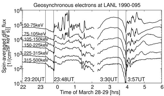
The Los Alamos geostationary spacecraft 1990-095 tra-versed the pre-midnight region (∼21:00 MLT) at the time of the first activation onset. Figure 3 shows the electron data from the spacecraft 1990-095. The electron fluxes started to decrease at 23:20 UT, which coincides with the time of the southward IMF arrival at the magnetopause. At 23:48 UT a

sharp increase in the electron fluxes was recorded, consistent with the timing of the negative bay onset in the ground mag-netometer data (23:45 UT). The geostationary electron data support the global picture of a substorm sequence: At the time of the arrival of the southward IMF the tail field started to stretch in the nightside, as evidenced by the decrease in the electron flux at geostationary orbit near midnight. The injection marked the onset of the substorm expansion phase, consistent with the ground magnetometer recordings.

At 03:30 UT, the spacecraft 1990-095, now traversing near the midnight meridian (∼01:00 MLT), again recorded a de-crease in the electron fluxes. At 03:57 UT, another sharp increase in the electron fluxes occurred. The data presented suggest that the 04:00 UT event is consistent with the pic-ture of a magnetospheric substorm, as evidenced by a flux decrease that indicates tail stretching, and geostationary in-jection and northward propagation of the negative bay on the ground that indicates dipolarization of the tail magnetic field. 2.3 Global ionospheric observations

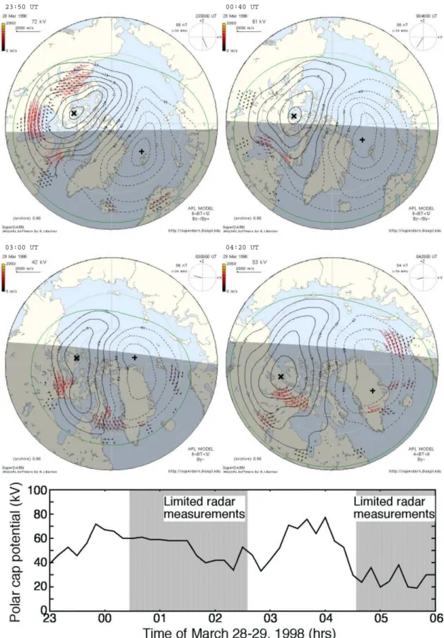
Figure 4 presents the Northern Hemisphere instantaneous convection patterns as measured by the SuperDARN radars (Greenwald et al., 1985). The convection patterns are shown at the onset (23:50 UT) and maximum of the first substorm (00:40 UT), during the activity minimum between the sub-storms (03:00 UT), and close to the maximum of the second substorm (04:20 UT). The bottom panel of Fig. 4 gives the polar cap potential determined from SuperDARN measure-ments. At 23:50 UT the dusk convection cell is well-defined by the SuperDARN radar measurements, whereas the dawn cell has insufficient data coverage. The polar cap potential inferred from the radar measurements is 72 kV. At the max-imum of the first substorm, 00:40 UT, both dusk and dawn cells have insufficient data coverage, although some convec-tion features are fairly well-defined by measurements. There-fore, the polar cap potential (61 kV) at 00:40 UT is deter-mined by a statistical model (e.g. Ruohoniemi and Baker, 1998 and references therein), which tends to underestimate the instantaneous potential (M. Ruohoniemi, private com-munication, 2004). At the minimum between the substorms (03:00 UT), and near the maximum of the second substorm (04:20 UT) the SuperDARN radars define the convection pat-tern again fairly well. The polar cap potentials were 42 kV and 53 kV, respectively. In conclusion, except for the max-imum of the first substorm (00:40 UT), the convection pat-tern and the polar cap potential determined from the Super-DARN radars are quite reliable during the time period shown in Fig. 4.

22

23

0

1

2

3

4

5

6

10

10

10

10

10

10

50-75keV

75-105keV 105-150keV 150-225keV 225-315keV 315-500keV

23:20UT

23:48UT

3:30UT

3:57UT

Time of March 28-29 [hrs]

Geosynchronous electrons at LANL 1990-095

Spin-averaged dif

f. flux

[1/(cm

2

sr keV s)]

Fig. 3.Geostationary electron observations.

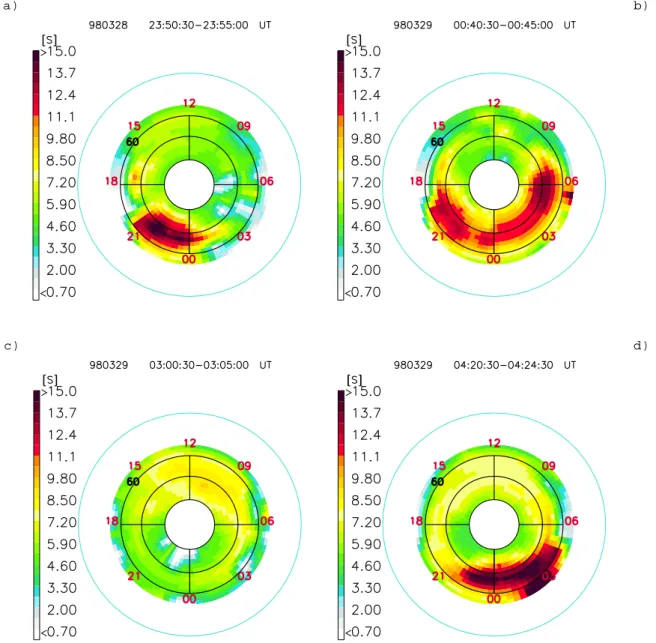
substorm (Fig. 5a) the pre-midnight sector shows enhanced Pedersen conductance, verifying that the onset timing deter-mined from the ground magnetometer data (Fig. 2) is correct, because the GHB station is located below the enhanced con-ductance region. At maximum, the Pedersen concon-ductance, using the Aksnes et al. (2002) method, is more than 15 S, while on average the conductance is 4–10 S along the oval. Figure 5b indicates that at the maximum of the first substorm the enhanced conductance extends over the nightside, while the average Pedersen conductance is∼10 S. In between the two substorms (Fig. 5c) the nightside conductance has de-creased to∼4–6 S. The second substorm took place in the post-midnight sector, as indicated by the locations of the Ped-ersen conductance maxima (Fig. 5d). This confirms the tim-ing of the second substorm ustim-ing the ground magnetometers located in the dawn sector (Fig. 2). At maximum activity, the Pedersen conductance is over 15 S, although variable be-tween 6–10 S along the nightside oval.

3 Joule heating from different methods 3.1 Spatial variation

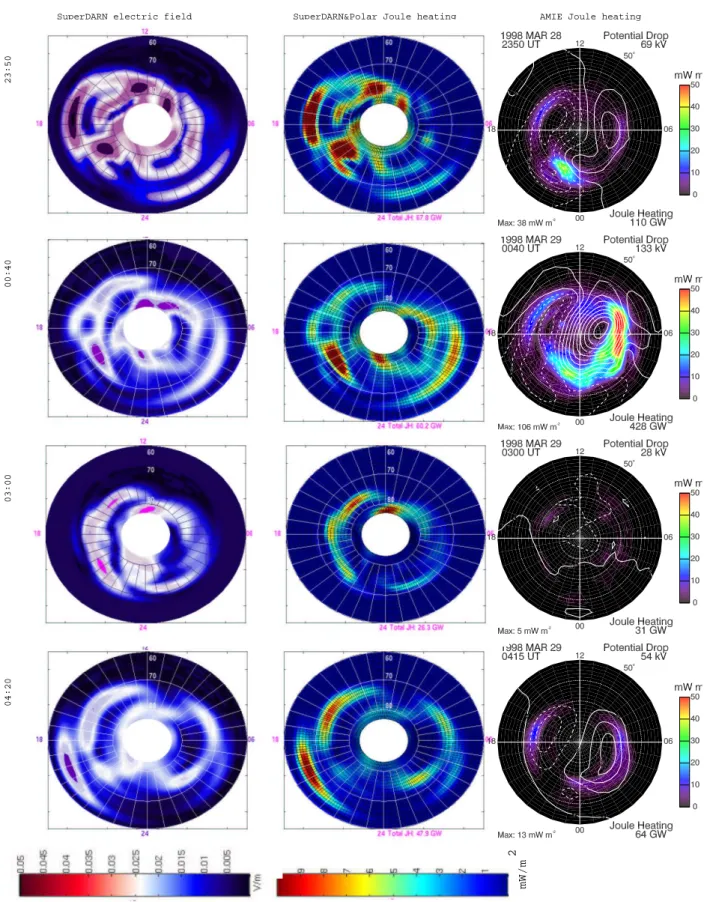
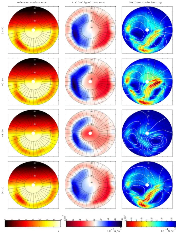
Figure 6 shows data from the onset and maximum of the first substorm (23:50 and 00:40 UT, first two rows), mini-mum in between the substorms (03:00 UT, third row), and near the maximum of the second substorm (04:20 UT, last row). In each plot, 12:00 MLT is up, 24:00 MLT is down and 18:00 (06:00) MLT is to the left (right); white grid lines indicate the magnetic latitude. The first column presents the global electric fields as measured by the SuperDARN radars. These electric fields may include large errors during insuf-ficient radar data coverage. Furthermore, as the potentials

are fitted to the radar data using a spherical harmonic fitting procedure, a residual potential sometimes appears equator-ward of the zero potential line. To avoid overestimating the Joule heating due to the residual electric field, we have forced the electric field to be zero equatorward of the zero potential line. The second column gives maps of Joule heating, com-puted by taking the electric field from the SuperDARN radars and the Pedersen conductance from the Polar measurements (Fig. 5), which are first interpolated to have the spatial reso-lution of the SuperDARN electric fields. Hereafter, this Joule heating is termed “the observed Joule heating”. The last col-umn gives the instantaneous Joule heating as computed from the AMIE procedure. The polar cap potential is overlaid on the AMIE Joule heating maps as white contours.

23:50 UT

04:20 UT 03:00 UT

00:40 UT

a) b)

c) d)

Fig. 5.Pedersen conductance maps derived from measurements by the UV and X-ray imagers on board the Polar satellite for the time periods of(a)23:50–23:55 UT,(b)00:40–00:45 UT,(c)03:00–03:05 UT, and(d)04:20–04:25 UT.

At the maximum of the first substorm, at 00:40 UT, the AMIE polar cap potential is 132 kV, while SuperDARN sug-gests 61 kV. The latter is probably an underestimation due to insufficient data coverage (see Fig. 4b). Statistically, forKp

4.7 at 00:40 UT the polar cap potential is∼90 kV, as sug-gested by the empirical polar cap potential proxy of Boyle et al. (1997). The SuperDARN and Polar measurements show a maximum at∼20:00 MLT (17 mWm−2). However, on av-erage the observed Joule heating is∼2 mWm−2throughout the Northern Hemisphere. On the other hand, the AMIE re-sults show that the Joule heating is largely concentrated on the dawnside Region 1 and Region 2 current closure region, although some Joule heating also appears on the nightside. The AMIE maximum is 106 mWm−2_.

In between the two substorms, at 03:00 UT, the AMIE po-lar cap potential has decreased to 27 kV, while SuperDARN radars suggest 42 kV. The observed Joule heating is now 10 mWm−2_{at maximum (dayside poleward edge), while on} average the Joule heating is∼1 mWm−2_{throughout the oval.} The observed Joule heating is enhanced on the dusk oval. On the other hand, the AMIE procedure yields virtually no Joule heating (maximum∼5 mWm−2). Near the maximum of the second substorm, at 04:20 UT, the polar cap potential is 54 kV in AMIE, while SuperDARN radars obtain 53 kV. Generally, the spatial variation of the observed Joule heat-ing agrees with the AMIE results, as both show enhanced Joule heating at the vicinity of 70◦ _{on virtually all MLTs.}

SuperDARN electric field SuperDARN&Polar Joule heating AMIE Joule heating

00:40

03:00

04:20

23:50

mW/m

2

at∼20:00 MLT. The maximum of the observed Joule heat-ing is now 11 mWm−2, but on the average∼1 mWm−2. The AMIE maximum during that period is 12 mWm−2.

3.2 Total integrated Joule heating

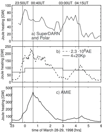
Figure 7 presents the total Joule heating integrated over the Northern Hemisphere computed using various methods dur-ing the 28–29 March 1998 event. In Fig. 7a, Joule heatdur-ing is computed by taking the global electric field from Super-DARN radars (Fig. 6), while the Pedersen conductance is taken from the Polar global imagers (Fig. 5). Thus, Fig. 7a presents the integration of the observed Joule heating in Fig. 6; the 10-min spatial resolution is due to the integration of UVI and PIXIE instruments used in deriving the Peder-sen conductance. Figure 7b gives estimates of the integrated Joule heating rate based on AE (Ahn et al., 1983) andKp

indices (Foster et al., 1983), while Fig. 7c gives the total Joule heating as computed by the AMIE procedure. Ahn et al. (1983) used radar and ground magnetic field measure-ments to develop global conductance distributions, which were then used to compute the electric field distributions with the method introduced by Kamide et al. (1981). Sep-arate equations were given for the standard AE index (based on 12 magnetometers) and for an AE index derived from a larger number of magnetometers. Figure 7 shows the Ahn et al. (1983) proxy for the standard AE index. Regardless of the poor temporal resolution, the Foster et al. (1983) proxy PJ H(GW )=4+20Kp at equinoxes gives an estimate of the

level of Joule heating based on the most comprehensive sta-tistical study published up to date. The vertical lines cor-respond to Fig. 4, Fig. 5, and to instantaneous global maps presented in Fig. 6.

As indicated in Fig. 4, the SuperDARN radars have insuf-ficient data coverage during 00:30–02:30 UT, and therefore both the temporal variation and the magnitude of the Joule heating in Fig. 7a during this period include large uncertain-ties. Compared to the AE-proxy in Fig. 7b, the onset of the second substorm occurs slightly earlier (later) in the observed Joule heating (AMIE), indicating that the various methods do not have a one-to-one correspondence in terms of temporal evolution. In terms of magnitude of the total Joule heating, the best correspondence is obtained during the second sub-storm, when the observed Joule heating, the AE-proxy, and the AMIE results are in quantitative agreement, given that the error estimate of the Ahn et al. (1983) proxy is±50%. Dur-ing the first substorm, the Joule heatDur-ing from the different methods are far from a quantitative agreement: The AMIE results show twice as large values as compared to the AE-proxy, which shows twice as large values as compared to the Kp-proxy and the observed Joule heating.

4 GUMICS-4 global MHD simulation

GUMICS-4 (Janhunen, 1996) is a computer simula-tion designed specifically for solving the coupled solar

0 100 200 300 400 500

Joule heating [GW]

c) AMIE

23 0 1 2 3 4 5 6

time of March 28-29, 1998 [hrs] 0

50 100 150 200 250

Joule heating [GW]

23:50UT 00:40UT 04:15UT

b) 2.3 .108AE 4+20Kp

03:00UT

0 20 40 60 80 100

a) SuperDARN and Polar

Joule heating [GW]

Fig. 7.Global integrated Joule heating in the Northern Hemsiphere as given by(a)SuperDARN and Polar measurements(b)AE- and Kp-based proxies, and(c)AMIE procedure during 28–29 March

1998. Vertical lines correspond to Fig. 6.

wind-magnetosphere-ionosphere system. The code consists of two computational domains: The MHD domain includ-ing the solar wind, and the magnetosphere and the electro-static domain including the ionosphere. The fully conserva-tive MHD equations are solved in a simulation box extending from 32REto−224RE in theXGSEdirection and±64RE

in theYGSE direction andZGSE direction. Near the Earth

the MHD simulation box reaches a spherical shell with a ra-dius of 3.7RE, which maps along the dipole field to

approxi-mately 60◦_{in magnetic latitude. The grid in the MHD}

simu-lation box is a Cartesian octogrid, and it is adaptive, meaning that whenever the code detects large spatial gradients, the grid is refined. Furthermore, in order to save computation time, the code uses subcycling (Janhunen et al., 1996), in which the time step varies with the local travel time of the fast magnetosonic wave across a grid cell. Solar wind den-sityρ, temperatureT, velocity v and magnetic fieldBare treated as boundary conditions along the sunward wall of the simulation box; outflow conditions are applied on the other walls of the simulation box.

A/m 2

S

GUMICS-4 Joule heating Field-aligned currents

Pedersen conductance

23:50

00:40

03:00

04:20

10-8 10-4W/m

2

Fig. 8. Northern Hemispheric GUMICS-4 Pedersen conductance, field-aligned currents, and Joule heating (white contours are polar cap potential isocontours) at 23:50 UT, 00:40 UT, 03:00 UT, and 04:20 UT.

magnetosphere using dipole field lines. The region between the ionosphere and the 3.7RE shell is a passive medium,

which only transmits electromagnetic effects, and where no currents flow perpendicular to the magnetic field. A triangu-lar finite element grid of the ionosphere is fixed in time, al-though refined to∼100 km spacing in the auroral oval region. The ionosphere-magnetosphere feedback loop includes the

recombination rates in 20 nonuniform height levels ranging from 64 km to 194 km. The electron densities are used in the calculation of the Pedersen and Hall conductivities, which are height-integrated to give the conductances at 110 km altitude. The dayside conductances are computed from F10.7 flux according to the empirical formulas of Moen and Brekke (1993), and 0.5 S is assumed to be the background conduc-tance originating from ion precipitation, galactic UV and X-rays, energetic neutral atoms, and UV and X-rays reflected from the Moon. The MSIS (Hedin, 1991) model is used for the thermospheric model, giving for example, the collision frequencies needed in the computation of the conductances. The ionospheric potential is solved by using the field-aligned currents as a source for the horizontal ionospheric currents, which in turn are defined by the height-integrated Ohm’s law in the ionosphere. The ionospheric potential is then mapped to the inner shell of the magnetosphere, where it is used as a boundary condition for the MHD equations. More infor-mation on the ionospheric computation can be found in Jan-hunen and Huuskonen (1993).

The 28–29 March 1998 event was simulated using Wind observations as an input to the code. The IMFBx was set

to zero to ensure a divergenceless input magnetic field. The smallest grid size in the simulation was set to 0.25RE. As

the neutral winds are not modeled in the simulation, the GUMICS-4 Joule heatingPJ H Gis calculated as

PJ H G=

Z 90

0

6PE2dS, (3)

where the electric field and the Pedersen conductances are determined in the ionosphere;dSis the area element of the ionosphere and the integration is carried out over the North-ern Hemisphere (between 0◦_{and 90}◦ _{in magnetic latitude),}

although usually the Joule heating in GUMICS-4 is concen-trated poleward of∼50◦_.

Figure 8 presents global maps of the GUMICS-4 Peder-sen conductance, field-aligned currents, and Joule heating at 23:50 UT, 00:40 UT, 03:00 UT, and 04:20 UT; in each plot the orientation is as in Fig. 6, and the latitude grid is indicated as black contours. The onset is characterized as enhanced Pedersen conductance in the 21:00 MLT sector, consistent with the measurements made by the Polar global imagers (cf. Fig. 5). However, the magnitude of the GUMICS-4 Pedersen conductance at the oval (∼5 S) is lower than what is observed (∼12 S, Fig. 5). Region 1 currents are enhanced, whereas the Region 2 currents are weak in the dusk and dawn sectors. The polar cap potential pattern is similar to the observed pattern in Fig. 4, as the convection cells are tilted towards the dawn. Furthermore, the GUMICS-4 Joule heating pattern has simi-larities with the observed Joule heating in Fig. 6, as the oval ranging from the dusk to postmidnight, and the polar cap in between the convection cells show enhanced heating. The magnitude of GUMICS-4 Joule heating is much lower than the observations show in Fig. 6.

Near the maximum of the first substorm, at 00:40 UT, the GUMICS-4 Pedersen conductance has remained essentially

23

0 5 10

24 01 02 03 04 05 060

50 100

GUMICS-4

Joule heating [GW]

observed

Joule heating [GW]

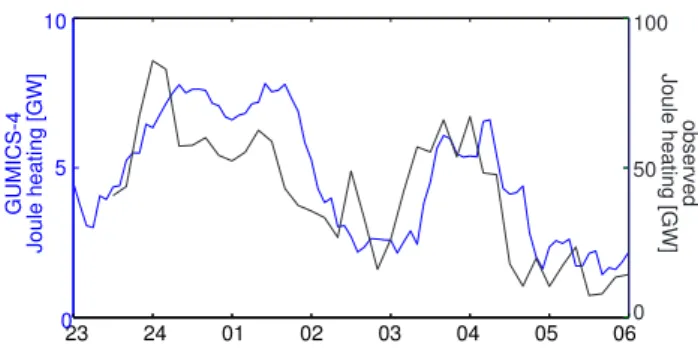
Fig. 9. (left axis, on blue) Total integrated Northern Hemispheric Joule heating in the GUMICS-4 simulation. (right axis, on black) Total integration of Joule heating computed from SuperDARN elec-tric fields and Polar measurements of Pedersen conductance.

similar as during the onset, whereas the Region 1 currents have intensified. Joule heating is also enhanced compared to the onset conditions; however, the heating occurs essen-tially in the same regions (oval and polar cap in between the convection cells) as during the onset. Also, the observed Joule heating in Fig. 6 shows this behavior, as both the oval and the polar cap show enhanced heating. At the minimum between the substorms, at 03:00 UT, the Pedersen conduc-tance, field-aligned currents and Joule heating have all de-creased. Although at 03:00 UT the IMFzcomponent is posi-tive, the NBZ current system is not fully developed, possibly because of a simultaneous considerable IMF y component that moves the reconnection regions towards lower latitudes (Kallio and Koskinen, 2000). A fully developed NBZ cur-rent system, where a negative field-aligned curcur-rent is gen-erated in the dawnside high latitudes, is observed later in the GUMICS-4 results as the IMF clock angle is more purely ori-ented northward. Joule heating, however, continues to show the same morphology as before: the faint maxima of heating occur at the oval and in between the convection cells, con-sistent with the observed Joule heating in Fig. 6. Near the maximum of the second substorm, at 04:20 UT, the obser-vations show that the Pedersen conductance is enhanced in the post-midnight region (Fig. 5), whereas the GUMICS-4 results show the enhanced Pedersen conductance in the pre-midnight region. Nevertheless, the field-aligned currents and the Joule heating are again enhanced, and again consistent with the observed Joule heating; the heating occurs at the oval and in between the convection cells where the electric field is increased.

Table 1.Estimates of total Joule heating for the 28–29 March 1998 event using different techniques.

23:50 00:40 03:00 04:20

UT UT UT UT

J HAhn[GW] 142 175 31 103

J HAMI E[GW] 110 428 31 68

< J Hobs >[GW] 68 60* 26 48

J HGU MI CS[GW] 5.5 7.6 3 6.6

*Affected by insufficient radar data coverage

show a somewhat simultaneous increase and decrease dur-ing the first substorm. The second substorm onset in the GUMICS-4 results occurs slightly later than in the observed Joule heating; however, the second onset is simultaneous in the GUMICS-4, AE-proxy and AMIE results, although the GUMICS-4 (AMIE) Joule heating increases faster (slower) than the AE-proxy (Fig. 7). Figure 7 shows that the first substorm has two intensifications; this double-peak property of the total Joule heating is also captured by the GUMICS-4 simulation. The relative amplitude of the GUMICS-GUMICS-4 in-tensifications is similar to those in the AE-proxy: the Joule heating level during the second substorm is about two-thirds of the first substorm. Figure 9 clearly suggests that the mag-nitude of GUMICS-4 Joule heating is quite consistently a factor of 10 smaller than the observed Joule heating. This is also in accordance with the magnitude of the Foster et al. (1983) proxy.

Table 1 presents the summary of Joule heating estimates from the Ahn et al. (1983) proxy, AMIE, SuperDARN and Polar measurements, and GUMICS-4, respectively. The ob-served Joule heating at 00:40 UT is most probably underes-timated since the statistical method used to derive the con-vection pattern underestimates the polar cap potential during insufficient data coverage of the SuperDARN radars. The most distinctive feature of Table 1 is that the different Joule heating estimates are relatively closer together towards the end of the substorm period, and that the relative differences among the various estimates during the maximum of the first substorm is large.

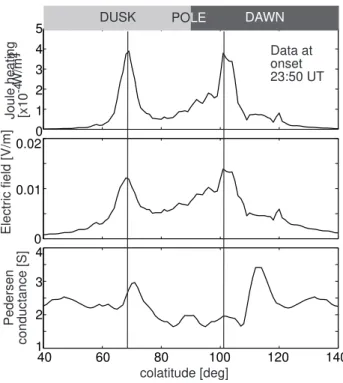
5 Theoretical aspects on estimating Joule heating In general, conductance and electric field are spatially anti-correlated, such that electric fields tend to circumvent regions of high conductance (e.g. Evans et al., 1977; Mallinckrodt and Carlson, 1985). In the case of perfect spatial anticor-relation of electric fields and conductance, no Joule heating would be produced, since no charge carriers would carry electric current along the electric field. In the ionosphere, however, the global convection electric field and ionization due to precipitation and EUV radiation ensure that generally electric fields and regions of high conductance overlap spa-tially. Therefore, in the large scale the electric fields and

0 1 2 3 4 5

0 0.01 0.02

1 2 3 4

Joule heating [x10

-4

W/m

2]

Electric field [V/m]

Pedersen

conductance [S]

colatitude [deg]

DUSK POLE DAWN

Data at onset 23:50 UT

40 60 80 100 120 140

Fig. 10.GUMICS-4 Joule heating, electric field and Pedersen con-ductance along the terminator at 23:50 UT.

conductance are correlated in the sense that both exist glob-ally in the ionosphere.

In smaller scales, the average of the global electric field and conductance may overestimate the true Joule heating in regions where electric fields and conductances are spatially anticorrelated. In fact, it can be shown (see Appendix A) that under the anticorrelation assumption

AiσiEi2>

Z

Ai

σ (x)E(x)2d2x, (4) where the right-hand-side of Eq. (4) denotes the true Joule heating in areaAi, and the left-hand-side denotes the Joule

heating obtained from independent averaged measurements of the electric field Ei and conductance σi. The relation

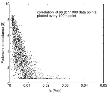
in the simulation is not only a property of the one time in-stant plotted in Fig. 10, Fig. 11 presents the electric field and Pedersen conductance data pairs taken at random loca-tions over the Northern Hemisphere poleward of 60◦during 23:30–06:00 UT, such that each data point corresponds to a location and time in the simulation ionosphere. Since the whole data set contains over 277 000 values, we plot only every 100th datapoint. Clearly, Fig. 11 suggests that in the simulation the Pedersen conductance is on average low on locations where the electric field is high, and vice versa. The correlation coefficient is −0.66 in both the plotted subset and the large data set (277 000 data points). Notice that in Fig. 11 the lowest conductance values (0.5) result from the background conductance.

Theoretically, the overestimation of Joule heating due to independent measurements of the electric field and conduc-tance may be infinite. For example, elementAi may include

piecewise defined asynchronous step functions of the elec-tric field and conductance such that, for example,Ei varies

between 0 and 2 mV/m, while conductance varies between 2 and 0 S. Therefore the averages of the electric field and con-ductance yield 1 mW/m2 _{for Joule heating inA}

i, although

the true Joule heating would be 0 mW/m2_{. Assessment of} the overestimation of Joule heating (Pcorr) due to spatial

an-ticorrelation ofEand6P can be computed using the

corre-lation coefficient and standard deviations ofE2and6P (see

Appendix A) as

Pcorr=|Corri|ST DσST DE2, (5) where Corri ∈ [−1,0]andST Dσ andST DE2 are standard

deviations of Pedersen conductance and the square of the electric field, respectively, in an area elementAi. A global

estimate of the correction to Joule heating due to spatial an-ticorrelation would therefore require measurements ofEand 6P with high spatial resolution over the Northern

Hemi-sphere.

One possible situation where the above arguments (Joule heating is overestimated due to spatial anticorrelation of E and 6P) are not valid is related to the so-called

Cowling channel (e.g. Bostr¨om, 1974) of the polarization electric field. Namely, if a primary (convection) electric field is aligned with a slab of higher conductance (such as an auro-ral arc), a secondary electric field driving secondary currents appears at the ends of the slab. These secondary currents carry Joule heating, and the higher the conductance in the slab, the higher the secondary current and hence the higher the Joule heating. Thus, in this case the electric field and conductance are correlated, which increases the Joule heat-ing. However, the convection electric field is parallel to the auroral arc generally only in the nightside. On the other hand, for example, Marklund et al. (2001a) found that in the auro-ral bulge the secondary electric field is efficiently closed by local field-aligned currents, thus making the Cowling chan-nel model inadequate to describe the phenomena related to the substorm current wedge.

0 0.01 0.02 0.03 0.04 0.05 0

2 4 6 8 10

E (V/m)

Pedersen conductance (S)

correlation -0.66 (277 000 data points) plotted every 100th point

Fig. 11. Electric field versus Pedersen conductance over the time period of 23:30–06:00 UT in the GUMICS-4 simulation. Each point correspond to a time and location above 60◦; locations are obtained randomly over all MLT’s. Correlation coefficient is−0.66. To re-duce data in the plot, only every 100th point is plotted (for those points, correlation is also−0.66).

6 Discussion and conclusions

In this paper we have estimated the Northern Hemisphere Joule heating with various techniques during a substorm event of 28–29 March 1998, aiming to quantitatively esti-mate the ability of GUMICS-4 global MHD simulation to predict ionospheric Joule heating. The purpose of this work is to calibrate the total ionospheric power consumption equa-tion (Palmroth et al., 2004a) given by Eq. (2). As was men-tioned earlier, Palmroth et al. (2004a) showed that Eq. (2) was able to predict the ionospheric total power consump-tion in the simulaconsump-tion from solar wind parameters with more than an 80% correlation coefficient. Since in the simula-tion both the Joule heating and precipitasimula-tion were in tem-poral agreement with the AE index, it was argued that the right-hand side of Eq. (2) could roughly predict the temporal behavior of ionospheric power dissipation as determined by the AE-proxies. Although the components ofPionosphere in

Eq. (2) yielded lower ionospheric power dissipation as com-pared to the AE proxies, Palmroth et al. (2004a) speculated that Eq. (2) could still be used to predict ionospheric power dissipation if the constantCin Eq. (2) was scaled to account for the “missing” ionospheric power in the GUMICS-4 sim-ulation.

energy fluxρv3multiplied by a term characterizing the IMF zeffect, i.e. reconnection. The approximateρv3behavior of Eq. (2) is supported by a statistical survey carried out by Ols-son et al. (2004), who found that total ionospheric Joule heat-ing is highly correlated with solar wind kinetic energy flux ρv3. This agreement between the instantaneous GUMICS-4 results and the statistical results by Olsson et al. (200GUMICS-4) suggests that GUMICS-4 Joule heating is in accordance with the system behavior over longer time periods. We now focus on the scaling ofC in the following way: First, we evalu-ate whether GUMICS-4 Joule heating follows temporally the Joule heating occurring in the ionosphere during this event. Second, we estimate roughly the correct magnitude of Joule heating during the event. Third, we discuss the physical problems associated with the scaling and whether the scaling of GUMICS-4 results leads to a reasonable estimate of global Joule heating. Finally, we discuss whether the calibration of Eq. (2) is successful as far as Joule heating is concerned. A similar calibration of the precipitation power will be carried out in a future investigation.

Although at global scales the Pedersen conductance is al-most constant in time due to the large contribution of the day-side EUV radiation, Fig. 5 shows that at auroral latitudes the precipitation governs the spatial distribution of Pedersen con-ductance. However, Joule heating depends quadratically on the electric field. Therefore, the temporal variation of the to-tal hemispheric Joule heating most probably follows the tem-poral variation of the global electric field, and consequently the polar cap potential. The polar cap potential difference has been found to be linearly proportional to the AE index (Ahn et al., 1984; Weimer et al., 1990), and therefore the temporal variation of the polar cap potential should follow that of the AE index (Fig. 2). Hence, the temporal variation of the AE proxy presented in Fig. 7 gives most probably also the tempo-ral variation of the total integrated Joule heating. As was seen from Fig. 9, the temporal evolution of the GUMICS-4 Joule heating is well-correlated with that of the AE index. This is not a new result: in all events simulated with GUMICS-4 to date, the total integrated Joule heating follows the temporal variation of the AE index. It is thus likely that the temporal evolution of the global integrated Joule heating in the North-ern Hemisphere is well reproduced by the GUMICS-4 global MHD simulation. However, the level of Joule heating in all the simulated events, the present event included, appears to be less than suggested by, for example, the AE-proxies.

Although the Foster et al. (1983) statistics were binned us-ing theKpindex, which has a poor temporal resolution, the

results are based on the most comprehensive statistical sur-vey published to date, in which the data are gathered from direct measurements on board the AE-C spacecraft. Fur-thermore, to our knowledge, the Foster et al. (1983) paper is the only statistical study using measurements of6P and

E in which the spatial anticorrelation of the electric field and Pedersen conductance is taken into account, as Foster et al. (1983) measure the two parameters simultaneously using the same satellite recordings. Therefore, the magnitude of global Joule heating may not be overestimated in the original

database, although theirKp-proxy may sometimes

underes-timate the Joule heating due to the poor temporal resolution of theKp. Olsson et al. (2004) carried out another statistical

survey on the Northern Hemisphere field-aligned Poynting flux using the Astrid-2 satellite electric and magnetic record-ings on∼3000 orbits. They found a rather good agreement with the Foster et al. (1983) results, although strictly speak-ing the Poyntspeak-ing flux includes the energy drivspeak-ing both Joule heating and neutral winds, whereas the Foster et al. (1983) results deal with6PE2only. Nevertheless, the agreement is

worth noticing, particularly because the direct Poynting flux measurements naturally do not include any overestimations due to multiplication of the averaged electric fields and Ped-ersen conductances from different sources. Furthermore, the two statistical surveys are carried out using satellite record-ings utilizing different types of instruments (double probes on board Astrid-2, and electric field and ion drift meter on board AE-C), and the time resolutions are different (1 s for Astrid data and 15 s for AE-C data). Therefore, the Olsson et al. (2004) results are to be taken as strong evidence that the much larger data set of Foster et al. (1983) gives the6PE2

more or less correctly. On the other hand, the Olsson et al. (2004) results are also in accordance with theρv3behavior of Eq. (2).

For the present event, theKpproxy of Foster et al. (1983)

suggest Joule heating values below 100 GW for the Northern Hemisphere. The global observations during this event sug-gest∼70 GW of Joule heating during the first onset, whereas the value during the first maximum (60 GW) is most likely to be an underestimation due to the lower radar data cov-erage. The Ahn et al. (1983) Joule heating proxy suggests

∼200 GW at the peak of the first substorm, while AMIE sug-gests∼400 GW. Evidently, the large scatter among the differ-ent Joule heating estimates adds confusion as to what value should be used when quantitatively calibrating the power law of Eq. (2). However, Figure 7 and Table 1 suggested that the different estimates of Joule heating agree quantitatively towards the end of the substorm sequence. Figure 9 sug-gests that during the second substorm the GUMICS-4 result multiplied by 10 is in quantitative agreement with the ob-served Joule heating, which does not suffer from poor radar data coverage at that time period. With a factor of 10 lower, the GUMICS-4 Joule heating result is also consistent with the AMIE Joule heating from 02:30 UT onwards, although during the maximum of the first substorm the AMIE results show quite large Joule heating rates. Given that the error es-timate of the Ahn et al. (1983) proxy is ±50%, the lower limit of the AE-proxy is also consistent with the lower than 100-GW estimate. Hence, three of the four estimates for Joule heating presented in this paper essentially agree with each other during the course of the event, while all estimates agree with each other during the latter part of the simulated period. This leads us to conclude that the “true” hemispheric Joule heating during the 28–29 March 1998 substorm is be-low 100 GW at maximum, and the temporal variation folbe-lows that of the AE index.

seem disturbing prima facie, particularly when considering that the global MHD simulations do not generally include the neutral winds, and GUMICS-4 does not include the discrete arc physics as the parallel potential drop is set to zero in the current version. However, for example, Lu et al. (1995) esti-mate that the neutral winds take up to 6% of the electromag-netic energy. This is further supported by the quantitative agreement of the Foster et al. (1983) and Olsson et al. (2004) results, where the energy of neutral winds are excluded in the former but included in the latter. The fact that the two statis-tical surveys are in quantitative agreement indicates that the neutral winds do not consume large portions of the electro-magnetic energy statistically, although they may be impor-tant during individual events (Thayer, 1998). Furthermore, Wiltberger et al. (2004) showed that the Joule heating stays essentially the same whether or not it was calculated from a global MHD simulation coupled to a simulation modeling the thermospheric neutral winds. Therefore, it is likely that the lack of neutral winds in GUMICS-4 is not a severe draw-back as far as the total integrated Joule heating is concerned. It is not clear, however, how the discrete arc physics would affect the global Joule heating. Namely, if the current associ-ated with discrete arcs closes primarily locally, the potential difference over which the current closes would be small. In this case the global Joule heating may remain unaffected or decrease. On the other hand, if the return current region ad-jacent to the discrete arc has a very small conductivity due to escaping electrons (Marklund et al., 2001b), the Joule heat-ing associated with the global horizontal current would in-crease. Therefore, since the effect of the discrete arcs to global Joule heating is not resolved, it is unclear what their effect is on the GUMICS-4 results. Essentially, the scaling of GUMICS-4 results by a constant factor can be justified by the good reproduction of the global electric field. This can be seen in Fig. 12, which shows that the polar cap poten-tial is well-reproduced temporally in the GUMICS-4 simu-lation, given that there are also uncertainties in the temporal variation of the SuperDARN measurements due to the oc-casinal lower data coverage. As the magnitude difference between the GUMICS-4 polar cap potential with the Super-DARN measurements during good data coverage is always quite close to what is observed in Fig. 12, we have reason to believe that the scaling factor is also similar in other events.

We conclude that the GUMICS-4 Joule heating multi-plied by a factor 10 to achieve an agreement with obser-vational methods also asserts that the obserobser-vational meth-ods may overestimate Joule heating during the maximum of the first substorm. As can be seen in Table 1, the scaling of the GUMICS-4 results by a factor of 10 yields an es-timate that agrees with the observational methods only to-wards the end of the simulated period. During the onset and the first maximum, even the scaled GUMICS-4 results are lower than the observational methods suggest. The rea-son for this may be that the observational methods do not take into account the anticorrelation effect, which is intrin-sically taken into account in the ionospheric computation of GUMICS-4 (Figs. 10 and 11). Equation (5) indicates that

23 24 01 02 03 04 05 06 20

25 30 35 40 45 50 55

GUMICS-4

PC potential [kV]

time of March 28-29, 1998 [hrs] 10 20 30 40 50 60 70 80

GUMICS-4 SuperDARN

SuperDARN

PC potential [kV]

Fig. 12. GUMICS-4 (SuperDARN) polar cap potential on the left (right) axis. Due to insufficient radar data coverage, the Super-DARN may underestimate the polar cap potential during the first substorm.

the overestimation made by estimating the Joule heating us-ing independent average measurements of6P andEdepends

on the standard deviations of these two variables. Sugino et al. (2002) presented 10 years worth of European Incoherent Scatter Radar (EISCAT) data for the electric fields and con-ductances. Among other issues, the Sugino et al. (2002) data set shows clearly that the larger the intensities of the electric fields and conductances are, the larger their standard devi-ations. It is clear that the magnitudes of the electric fields and Pedersen conductances are positively correlated with in-creasing magnetic activity. Therefore, Eq. (5) suggests that the overestimation of Joule heating due to spatial anticorrela-tion ofEand6P increases with increasing magnetic activity,

both in absolute and relative terms. In practice, this would in-dicate that Joule heating during intense substorms and storms would be overestimated, while during less intense times the observational methods would give better predictions of the Joule heating. Naturally this does not apply to the Foster et al. (1983) results that do take the anticorrelation effect into account (to the extent that their 15-s temporal resolution al-lows); however the poor temporal resolution of the Kp

in-dex may sometimes lead to situations where the Foster et al. (1983) proxy yields ambiguous Joule heating values.

The overestimation made by taking independent averages of electric field and Pedersen conductances over regions where the two parameters are spatially anticorrelated can be assessed quantitatively. Matsuo et al. (2003) estimated the electric field variability statistically at high latitudes using DE-2 satellite measurements. They found that near equinox the standard deviation of the electric field over high lati-tudes is rather steadily∼30 mV/m above 60◦_{MLAT, while}

one assumes that ST D_E2=(ST DE)2, over the area

cov-ered in Matsuo et al. (2003), one obtains approximately 2 S·(0.03 V/m)2·1012m2 ≈1.8–4.5 GW in the case of per-fect anticorrelation (Corri=−1). If this value remains steady

over the high latitudes, over the ionosphere above 60◦_MLAT

(containing∼35 area elements of the size 1012_m2_{), the} to-tal value sums up to 63–153 GW, depending on the choice of the standard deviation of the Pedersen conductance (2 S or 5 S, respectively). For example, correlation coefficient of

−0.7 the above estimate would yield 44–107 GW. Therefore, the error made in estimating the total Joule heating by using independent averages of electric fields and conductances can become as large as the estimate itself.

Naturally the overestimation of total Joule heating due to spatial anticorrelation of6P andEapplies only over those

regions in the ionosphere where the electric field and conduc-tance are anticorrelated. As shown by Foster et al. (1983), this condition holds generally in the nightside, while there are regions adjacent to the cusp, where the electric field and conductance are spatially correlated. In the case of spatial correlation of the electric field and conductance, the Joule heating would actually be underestimated while ignoring the standard deviations of the two quantities. The total value of the overestimation or underestimation is affected not only by the values of the standard deviations, but also the total areas over which the quantities are spatially anticorrelated or cor-related, respectively. According to Foster et al. (1983), the region of spatial correlation of6P andEis generally smaller

than the area of spatial anticorrelation. Therefore, while in-tegrating over the whole Northern Hemisphere, ignoring the standard deviation would most probably still yield an over-estimation of the Joule heating. Note that this also applies to our estimate of the Joule heating based on global obser-vations: we took averages of the Pedersen conductance and the electric field from different sources, and therefore by def-inition this method yields an overestimation of Joule heating elsewhere except in the cusp region.

In conclusion we find that at any given time the GUMICS-4 estimate of the Joule heating during the 28–29 March 1999 event is 10 times less than the “true” Joule heating. The lesser amount of Joule heating in the GUMICS-4 global MHD sim-ulation is essentially caused by lower polar cap potentials and weaker Region 2 currents. As the closure of Region 1 and Region 2 currents to each other at the oval is the strongest source of Joule heating in the polar ionosphere (e.g. Gary et al., 1994; Olsson et al., 2004), the weaker Region 2 cur-rents in the MHD simulations lead to a situation in which smaller amounts of current close over the oval, decreasing the Joule heating associated with the Region 1 and Region 2 field-aligned current closure. The temporal evolution of Joule heating in GUMICS-4 is, on the other hand, consistent with the “true” Joule heating. To calibrate the power formula of Eq. (2), we find that as far as Joule heating is concerned, the constantCin Eq. (2) should be multiplied by a factor of 10. From the physics point of view, multiplying the simu-lated Joule heating by a constant is of course not satisfactory, but it helps us to obtain an estimate of the Joule heating in

cases where observational data are not available, for space weather prediction purposes, or in other cases where an esti-mate of the Joule heating is required.

Appendix A

Correlation and Joule heating in the averaging process Let σ (x) and E(x)2 be the conductance and square of the electric field in some domain A, respectively, and let P=R

Ad2xσ (x)E(x)2denote the corresponding Joule

heat-ing power. Consider idealised measurements of σ and E2 that amount to spatial averaging over small subdo-mains (grid cells)Ai of A, yielding the discrete quantities

σi≡(1/Ai)

R

Aiσ (x)d

2_{x and E}2

i ≡ (1/Ai)

R

AiE(x)

2_d2_x, i=1...N. We want to show that the Joule heating computed from the measurement data{σi, E2i},P˜≡

P

iAiσiE2i always

overestimates the true Joule heatingP ifσ andE2are anti-correlated in a subgrid scale, i.e. if

Corri≡

R

Aid

2_{x (σ (x)−σ}

i) E(x)2−E_i2

q R

Aidx (σ (x)−σi)

2qR

Aidx E(x)

2_−E2 i

2

<0 (A1)

in each grid celli=1...N. From Eq. (A1) it follows that 0>

Z

Ai

(σ (x)−σi)

E(x)2−E2_id2x

=

Z

Ai

σ (x)E(x)2−σ (x)E_i2−σiE(x)2+σiEi2

d2x

=

Z

Ai

σ (x)E(x)2d2x−E2_i Z

Ai

σ (x)d2x

−σi

Z

Ai

E(x)2d2x+AiσiEi2

=

Z

Ai

σ (x)E(x)2d2x−E2_iAiσi−σiAiEi2+AiσiEi2

=

Z

Ai

σ (x)E(x)2d2x−AiσiEi2 (A2)

from which it follows that AiσiEi2>

Z

Ai

σ (x)E(x)2d2x. (A3) Summing overiand using the definitions ofP andP˜ we ob-tainP >P˜ , i.e. that the Joule heatingP˜computed from aver-aged data yields an overestimation of the true Joule heating P if σ andE2 are anticorrelated in a subgrid scale in the sense of Eq. (A1).

We can solve the magnitude of the Joule heating overes-timation due to spatial anticorrelation ofEand6P. Using

Eq. (A2), Eq. (A1) can be written as Z

Ai

σ (x)E(x)2d2x=AiσiEi2

+Corri

s Z

Ai

dx (σ (x)−σi)2

s Z

Ai

As the square root terms on the right-hand side are essentially standard deviations ofσandE2, the magnitude of Joule heat-ing overestimationPcorrin areaAiis therefore calculated as

Pcorr=CorriST DσST DE2, (A5) where Corri ∈ [−1,0]andST Dσ andST DE2 are standard deviations ofσandE2, respectively, in areaAi.

Acknowledgements. The simulation input data were obtained through CDAWeb maintained by NSSDC. We are grateful to the WIND PI’s R. Lepping and K. Ogilvie who have agreed to distribute their data through CDAWeb. The SuperDARN data are summary data, which were obtained from the SuperDARN Data Archive lo-cated at http://superdarn.jhuapl.edu/index.html. We thank M. Ruo-honiemi and R. J. Barnes for making the SuperDARN data avail-able in the Internet. The work of M. Palmroth and P. Janhunen is supported by the Academy of Finland. The work of A. Aksnes is supported by the Research Council of Norway (NFR). We thank H. E. J. Koskinen for numerous fruitful discussions about the na-ture of Joule heating.

Topical Editor M. Lester thanks two referees for their help in evaluating this paper.

References

Ahn, B.-H. J., Akasofu, S.-I., and Kamide, Y.: The Joule heat pro-duction rate and the particle energy injection rate as function of the geomagnetic indices AE and AL, J. Geophys. Res., 88, 6275– 6287, 1983.

Ahn, B.-H. J., Akasofu, S.-I., Kamide, Y., and King, J. H.: Cross-polar cap potential drop and the energy coupling function, J. Geophys. Res., 89, 11028–11032, 1984.

Akasofu, S.-I.: Energy coupling between the solar wind and the magnetosphere, Space Sci. Rev., 28, 121–190, 1981.

Aksnes, A., Stadsnes, J., Bjordal, J., Østgaard, N., Vondrak, R. R., Detrick, D. L., Rosenberg, T. J., Germany, G. A., and Chenette, D.: Instantaneous ionospheric global conductivity maps during an isolated substorm, Ann. Geophys., 20, 1181–1191, 2002,

SRef-ID: 1432-0576/ag/2002-20-1181.

Bostr¨om, R.: Electrodynamics of the ionosphere, in: Cosmical Geo-physics, edited by: Egeland, A., Holter, Ø., and Omholt, A., Scandinavian University Books, Copenhagen, Denmark, 1974. Boyle, C. B., Reiff, P. H., and Hairston, M. R.: Empirical polar cap

potentials, J. Geophys. Res., 102, 111–125, 1997.

Evans, D. S., Maynard, N. C., Troim, J., Jacobsen, T., and Ege-land, A.: Auroral vector electric field and particle comparisons, 2, Electrodynamics of an arc, J. Geophys. Res., 82, 2235–2249, 1977.

Foster, J. C., St.-Maurice, J.-P., and Abreu, V. J.: Joule heating at high altitudes, J. Geophys. Res., 88, 4885–4896, 1983.

Fujii, R., Nozawa, S., Buchert, S. C., and Brekke, A.: Statistical characteristics of electromagnetic energy transfer between the magnetosphere, the ionosphere, and the thermosphere, J. Geo-phys. Res., 104, 2357–2365, 1999.

Gary, J. B., Heelis, R. A., Hanson, W. B., and Slavin, J. A.: Field-aligned Poynting flux observations in the high-latitude iono-sphere, J. Geophys. Res., 99, 11 417–11 427, 1994.

Gary, J. B., Heelis, R. A., and Thayer, J. P.: Summary of field-aligned Poynting flux observations from DE 2, Geo-phys. Res. Lett., 22, 1861–1864, 1995.

Greenwald, R. A., Baker, K. B., Hutchins, R. A., and Hanuise, C.: An HF phased array radar for studying small-scale structure in the high-latitude ionosphere, Radio Sci., 20, 63–79, 1985. Hedin, A. E., Extension of the MSIS tehermosphere model into the

middle and lower atmosphere, J. Geophys. Res., 96, 1159–1172, 1991.

Heelis, R. A. and Coley, W. R.: Global and local Joule heating ef-fects seen by DE 2, J. Geophys. Res., 93, 7551–7557, 1988. Janhunen, P.: GUMICS-3: A global ionosphere-magnetosphere

coupling simulation with high ionospheric resolution, in: Pro-ceedings of Environmental Modelling for Space-Based Applica-tions, Sept. 18–20, 1996, Eur. Space Agency Spec. Publ., ESA SP-392, 233–239, 1996.

Janhunen, P. and Huuskonen, A.: A numerical ionosphere-magnetosphere coupling model with variable conductivities, J. Geophys. Res., 98, 9519–9530, 1993.

Janhunen, P., Koskinen, H. E. J., and Pulkkinen, T. I.: A new global ionosphere-magnetosphere coupling simulation utilizing locally varying time step, in: Proceedings of Third International Con-ference on Substorms (ICS 3), Versailles, France, May 12–17, Eur. Space Agency Spec. Publ., ESA SP-389, 205–210, 1996. Kallio, E. J. and Koskinen, H. E. J.: A semiempirical

magne-tosheath model to analyze the solar wind-magnetosphere inter-action, J. Geophys. Res., 105, 27 469–27 479, 2000.

Kamide, Y., Richmond, A. D., and Matsushita, S.: Estimation of ionospheric electric field, ionospheric currents, and field-aligned currents from ground magnetic records, J. Geophys. Res., 86, 801–813, 1981.

Knipp, D. J., Emery, B. A., Engebretson, M., Li, X., McAllister, A. H., Mukai, T., Kakubun, S., Reeves, G. D., Evans, D., Obara, T., Pi, X., Rosenberg, T., Weatherwax, A., McHarg, M. G., Chun, F., Mosely, K., Codrescu, M., Lanzerotti, L., Rich, F. J., Sharber, J., and Wilkinson, P.: An overview of the early November 1993 geomagnetic storm, J. Geophys. Res., 103, 26 197–26 220, 1998. Lu, G., Richmond, A. D., Emery, B. A., and Roble, R. G.: Magnetosphere-ionosphere-thermosphere coupling: Effect of neutral winds on energy transfer and field-aligned current, J. Geophys. Res., 100, 19 643–19 660, 1995.

Lu, G., Baker, D. N., McPherron, R. L., Farrugia, C. J., Lum-merzheim, D., Ruohoniemi, J. M., Rich, F. J., Evans, D. S., Lepping, R. P., Brittnacher, M., Li, X., Greenwald, R., Sofko, G., Villain, J., Lester, M., Thayer, J., Moretto, T., Milling, D., Troshichev, O., Zaitzev, A., Odintzov, V., Makarov, G., and Hayashi, K.: Global energy deposition during the January 1997 magnetic cloud event, J. Geophys. Res., 103, 11 685–11 694, 1998.

Mallinckrodt, A. J. and Carlson, C. W.: On the anticorrelation of the electric field and peak electron energy within an auroral arc, J. Geophys. Res., 90, 399–408, 1985.

Marklund, G. T., Karlsson, T., Eglitis, P., and Opgenoorth, H. J.: Astrid-2 and ground-based observations of the auroral bulge in the middle of the nightside convection throat, Ann. Geophys., 19, 633–641, 2001a,

SRef-ID: 1432-0576/ag/2001-19-633.

Marklund, G. T., Ivchenko, N., Karlsson, T., Fazakerley, A., Dun-lop, M., Lindqvist, P.-A., Buchert, S., Owen, C., Taylor, M., Vaivads, A., Carter, P., Andr´e, M., and Balogh, A.: Tempo-ral Evolution of the Electric Field Accelerating Electrons Away From the Auroral Ionosphere, Nature, 414, 724–727, 2001b. Moen, J. and Brekke, A.: The solar flux influence on quiet time

Matsuo, T., Richmond, A. D., and Hensel, K.: High-latitude ionospheric electric field variability and electric potential de-rived from DE-2 plasma drift measurements: Dependence on IMF and dipole tilt, J. Geophys. Res., 108, (A1), 1005, doi:10.1029/2002JA009429, 2003.

Olsson, A., Janhunen, P., Karlsson, T., Blomberg, L. G., and Ivchenko, N.: Statistics of Joule heating in the auroral zone and polar cap using Astrid-2 satellite Poynting flux, Ann. Geophys., 22, 4133–4142, 2004,

SRef-ID: 1432-0576/ag/2004-22-4133.

Østgaard, N. and Tanskanen, E. I.: Energetics of isolated and stormtime substorms, in: Disturbances in Geospace: The Storm-Substorm Relationship, edited by: Surjalal Sharma, A., Kamide, Y., and Lakhina, G. S., Geophysical Monograph, 142, doi:10.1029/142GM14, 2003.

Palmroth, M., Janhunen, P., Pulkkinen, T. I., and Koskinen, H. E. J.: Ionospheric energy input as a function of solar wind parameters: global MHD simulation results, Ann. Geophys., 22, 549–566, 2004a,

SRef-ID: 1432-0576/ag/2004-22-549.

Palmroth, M., Pulkkinen, T. I., Janhunen, P., and Koskinen, H. E. J.: Ionospheric power consumption in global MHD simulation pre-dicted from solar wind measurements, IEEE Trans. on Plasma Sci., 32, 1511–1518, 2004b.

Palmroth, M., Pulkkinen, T. I., Janhunen, P., McComas, D. J., Smith, C., and Koskinen, H. E. J.: Role of solar wind dynamic pressure in driving ionospheric Joule heating, in press, J. Geo-phys. Res., 109, (A1), 1302, doi:10.1029/2004JA010529, 2004c. Pulkkinen, T. I., Ganushkina, N. Yu., Tanskanen, E. I., Lu, G., Baker, D. N., Turner, N. E., Fritz, T. A., Fennel, J. F., and Roeder, J.: Energy dissipation during a geomagnetic storm: May 1998, Adv. Space Res., 30, 2231–2240, 2002.

Raeder, J., Wang, Y., and Fuller-Rowell, T. J.: Geomagnetic storm simulation with a coupled magnetosphere-ionosphere-thermosphere model, in: Space Weather, edited by: Song, P., Singer, H. J., and Siscoe, G. L., Geophysical Monograph Series, 125, 377–384, 2001.

Richmond, A. D. and Kamide, Y.: Mapping electrodynamic fea-tures of the high-latitude ionosphere from localized observations – Technique, J. Geophys. Res., 93, 5741–5759, 1988.

Richmond, A. D.: Assimilative mapping of ionospheric electrody-namics, Adv. Space. Res., 12, 9–68, 1992.

Ridley, A. J., Richmond, A. D., Gombosi, T. I., De Zeeuw, D. L., and Clauer, C. R.: Ionospheric control of the magnetospheric configuration: Thermospheric neutral winds, J. Geophys. Res., 108, (A8), 1328, doi:10.1029/2002JA009464, 2003.

Ruohoniemi, J. M. and Baker, K. B.: Large-scale imaging of high-latitude convection with Super Dual Auroral Radar Network HF radar observations, J. Geophys. Res., 103, 20 797–20 811, 1998. Slinker, S. P., Fedder, J. A., Emery, B. A., Baker, K. B., Lum-merzheim, D., Lyon, J. G., and Rich, F. J.: Comparison of global MHD simulations with AMIE simulations for the events of May 19–20, 1996, J. Geophys. Res., 104, 28 379–28 395, 1999. Sugino, M., Fujii, R., Nozawa, S., Buchert, S. C., Opgenoorth, H. J.,

and Brekke, A.: Relative contribution of ionospheric conductiv-ity and electric field to ionospheric current, J. Geophys. Res., 107, (A10), 1330, doi:10.1029/2001JA007545, 2002.

Thayer, J. P., Vickrey, J. F., Heelis, R. A., and Gary, J. B.: Interpre-tation and modeling of the high-latitude electromagnetic energy flux, J. Geophys. Res., 100, 19 715–19 728, 1995.

Thayer, J. P.: Height-resolved Joule heating rates in the high-latitude E region and the influence of neutral winds, J. Geo-phys. Res., 103, 471–487, 1998.

Waters, C. L., Anderson, B. J., Greenwald, R. A., Barnes, R. J., Ruohoniemi, J. M.: High-latitude poynting flux from combined Iridium and SuperDARN data, Ann. Geophys., 22, 2861-2875, 2004,

SRef-ID: 1432-0576/ag/2004-22-2861.

Weimer, D. R., Maynard, N. C., Burke, W. J., and Liebrecht, C., Polar cap potentials and the auroral electrojet indices, Planet. Space Sci., 38, 1207–1222, 1990.