Co-movement between two processes with local persistence

｣ｾ＠

movement between two Processes with

Local Persistence

Luiz Renato Lima*

S

llmm

_er,

2001

Abstract

This paper introduces a residual based test where the null hypoth-esis of c:&InOvement between two processes with local ｰ･ｲｳｩｳｴ･ｮ｣ｾ＠ can

be tested, even under the presence of an endogenous regressor. It, therefore, fills in an existing lacuna in econometrics, in which long-run relationships can also be tested if the dependent and independent variables do not have a unit root, but do exhibit local persistence.

1

Introduction

According to Phillips et al

(2001),

a local persistence process exhibits a form of persistence in which shocks affect a variable for a long time but not forever. In particular, the effects of a shock may be highly persistent over a certain range, but may tend to disappear outside this range. Variables with local persistence have autoregressive coefficients near unity but are much more general than a a near-integrated process.!

Phillips (1986) proves that, in the presence of unit-root processes, infer-ence based on the t-statistic and F -statistic will be highly misleading. As

(1979, 1981)) and Phillips-Perron (Phillips and Perron (1988)) unit-root type of tests were largely used to test the null hypothesis of a unit root, whereas the KPSS (Kwiatkowski et al, (1992)),and Xiao (Xiao (1999)) unit-root type of tests offer a manner of testing stationarity (short-memory persistence) against the unit-root altemative. Hence, the decision on whether a time series is stationary or not was made based on tests whose null hypothesis corresponds to stationarity as we11 as on tests whose null corresponds to unit root. For example, if someone rejects the null hypothesis in the ADF test, but cannot reject it in the Xiao test, then the final conclusion would be that the time series is a stationary processo At the same way, one would believe that a time series would have a unit root if the null was rejected in the Xiao test and not rejected in the ADF testo However, although the literature on testing stationarity against a unit-root alternative (or vice versa) is relatively useful to deal with the 1(1)/1(0) dichotomy, it does seem to be useless to cap-ture the underlying dynamic of more complex time series. In fact, rejecting the null in both tests (ADF and Xiao) would lead us to an inconclusive re-sult. Another problem regarding unit-root tests is its low power over a range of processes with a root near unity (Elliot et al.,1996). H the time series has almost a unit root, then its degree of persistence will be high implying that one would hardly reject the null hypotheis of an exact unit root in the ADF test even if the economic variable had a root near unity but not necessary equal to one. In sum, conventional unit root test does not te11 much because the rejection of the unit root does not necessarily imply that the process is stationary and the non-rejection (or rejection of stationarity by the Xiao and KPSS tests) does not necessarily imply that the process is unit root.

of long-run equilibrium if there are variables with root near unity but not necessary equal to one.

Therefore, it turns out to be important to study comovement between variables with root near unity. In particular, the class of processes with local persistence introduced by Phillips et alo (2001) seems to be ideal for this purpose because ｬｯ｣｡ｬＭｴｾｵｮｩｴｹ＠ autoregressive coefficients are present in

the definition of local-persistence processes. Deriving a mechanism to test comovement between variables with local persistence will also be relevant because, as we will show later, spurious effects on the t-statistic will also arise if the variables display local persistence.

This paper seeks to derive a statistical test, through which the null hy-pothesis of stationarity may be tested consistently against the altemative hypothesis of local persistence. When applied to residual process of a linear regression, such test may be used to verify the validity of the null hypothesis of comovement between two processes with local persistence, even under the presence of a endogenous regressor. Limiting distribution of the test is de-rived under both the null and altemative, critical values are provided based on simulation experiments, and size and power of this test in a finite sample are also examined. We also show that local persistence yields spurious effects on the t-statistic, which implies that inference based on it will be misleading.

In order to illustrate the applicability of the test proposed in this paper, we consider two empirical applications. The first one investigates the validity of the hypothesis of forward exchange market unbiasedness, which states that the forward exchange rate is the best predictor of future spot exchange rate. The second application investigate the Fisher hypothesis on interest rate.

The paper is organized as follows: Section 2 presents the stochastic block local to unit process, developed by Phillips et al (2001). Section 3 re-exams the presence of spurious regression in time series with locall persis-tence. Section 4 introduces a residual based ｾｭｯｶ･ｭ･ｮｴ＠ test, and derives its asymptotic distribution under the null and altemative hypothesis.

Sec-tion 5 presents the results of the Monte Carlo experiment, secSec-tion 6 shows the empirical applications and section 7 concludes.

respectively, as the sample size, n, goes to infinite.

2

Stochastic Block Local To Unity Processes

2.1

Stochastic Block Local to Unity Process Without

Drift.

Consider the following block local to unity model first introduced by Phillips et al (2001) and represented by the system below

Yk,t - aYk,t-l

+

Uk,t,

tE

rm;k E

KK

(2.1)

Yk,l - Yk-l,m

c C

a

-

em '" 1

+ -,

c

<

O.

m

where

r

m

=

{l, ...

,m},

KK

=

{-K,-K

+

1, ... ,0,1, ... ,M}

with

K

>

O.

We have functionalized M and m on the sample size n, that is, m = nd

and M = n1_-d _with

°

_<

_d

<

_{1. Thus this system is characterized by a}

sequence of blocks with m observations in each block. We only observe

k

= 1, ... ,

M

blocks and, therefore, the observable time series correspond to

Yk,t with

t

E

r

m and k = 1, ... , M. The total sample is set equal to Mm = n

and, therefore, for any t and k, Yk,t equals to Y(k-l)m+t = Yi, i E In = (1, ... , n).

We have assumed that the localizing parameter is less than zero, c

<

0, which is supposed to be the same across blocks.

Given a fixed value of c

<

°

and a finite sample n, the intensity of persistence wi1l be completely determined by the magnitude of the parameter

d. Thus, the greater the value of d, the more persistent the autoregressive process 'Ui wi1l be inside each block. Also, notice that this model capture the whole evolution of a single time series Yi by setting the initial condition in

each block equal to the final observation in the previous one.

In each block of the system (2.1), the sequence of errors Uk,t follows a

linear process whose coeHicients satisfy the summability conditions with finite fourth moments. The specific structure of error generating mechanism is given by the assumption 1.

(a) ｻ￪ｴｽｾＭｯｯ＠ is a sequence of iid (0,1) variates with

E

lêtlP

<

00 for some p

>

4.

00

(b) Uk,t

=

Lbjêk,t-;, where êk,t

=

é(k-l)m+t. j=O

00

(c) LjGbj

<

00, for some a ｾ＠ 1,

j=O

(d) Let

w"

=

Ｈｾ｢［ｲ＠

and assume that infw"

>

O. (e) /bJ. =

w

2 and J.L4 =

w

4 existo

The imporlance of each condition above is as follows: The moment condi-tion in (a) and the summability condicondi-tion (c) guarantee that fourth moments of Uk,t are finite. Condition (c) also ensures the validity of a BN decompo-sition for Uk,t, for each k. ( see Phillips and Solo, 1992). The parameters /bJ. and J.L4 are long-run variance and square of the long-run variance.

Following Phillips et alo (2001) , one can show that:

The most imporlant results that stands out from this model and relevant for our purpose are the following:

(i/)

Local Stationarity

(d

= 1) : In this case n-!Yk,[mrJ

*

.Jl(r),

where

.Jl(r)

is the Ornstein Uhlenbeck processo H d

=

1, then Yi will asymptotically behave as a unit-root process and Yi = Op(n1/2_{), implying that the process} diverge as n ｾ＠ 00, at rate n1/2• In other words, when d

=

1, there is just one block, M

=

nO = 1, with m

=

n observations (the total sample) within that block. Thus, the entire time series, {Yà:=l' will asymptotically behave as a unit-root processo In finite sample,however, Yi will be stationary with autoregressive coefficient equal to a = 1

+

c/no Asymptotic theory for this kind of process was first introduced by Phillips (1987).2

(ii/)

Local Persistence (O

<

d

<

1) : In this case ｮＭｾｙｫＬＨｭｲｬ＠

*

m,c,

where

m,c

is a linear combination of independent difIusion processes as defined in Phillips et al (2001). In the presence of local persistence Yi will exhibit persistence inside each block k for a finite sample n, but it will ultimately diverge at rate nd/ 2 as n ｾ＠ 00. There are more than one block, that is M

=

n1_-d

>

_{1, with m}

=

_nd _{observations within each block. The partial}

2This process is more known by the name of near-integrated process or, more

sums inside each block will have nonstationary asymptotic behavior because a -+ 1 as n -+ 00, but partial sums over blocks still behave asymptotically like

a stationary system. In finite sample, however, Yi will be not only stationary but will also diplay persistency within many blocks.

(iii') (Standard) Stationarity (d

=

O). In this case Yi is

1(0),

that is,

n n-I

/2

E

Yi:::} B,,(r), where the limiting process B,,(r) is a Brownian motion

i=l

with variance ｷｾ＠ and Yi will be bounded even when

n

-+ 00. In other words,

when d = O, there will be M = n blocks (the total sample), with m =

nO = 1 observation within each block

(each

observation is a block itself). The coefficient "a" is, as in all cases, the same across blocks but never approach unity as it will in the local-persistence or local-stationary cases.

This is just a standard stationary case, in which the process is stationary both in finite and infinite samples.

Therefore, the first case

(d

= 1) corresponds to the local stationary pro-cess (or near-integrated propro-cesses) while the third case

(d

=

O) corresponds to the standard stationary processo The second case (O

<

d

<

1) is called

"local persistence" .

2.2

Stochastic Block Local to Unity Processes With

Drift.

Consider the following block local to unity model below

T

Yk,t - Tk,t

+

Yk,t, t E

r

m; k E KK (2.2)

Tk,t

-

ＧｐｾｔｫＬｴＬ＠ T k,t=(l,(k-l)m+t)'

Yk,t

-c c

aYk,t-1 + Uk,t, Yk,l

=

Yk-l,m, a

=

em '" 1

+

m' where c

<

O

Notice that the deterministic component, Tk,t, contains both a linear trend

t,

and a block specific component km, which guarantees the continuity of trend across blocks.The stochastic part represented by Eq. (2.7) corresponds to system (2.1), that is, it is a stochastic block local to unity processo

We estimate Yk,t from the residuals of the following regression

.,. -,.IT ｾ＠

where

CPll

is given by the following pooled regression formula

ｾ＠

m

]-1

ｾ＠

m ]

<P1I =

L

LT

k,t T'k,t

L L

T

ｫＬｴｙｾｴ＠

-1 t=1 1 t=1

(2.4)

Again, following Phillips et alo (2001), one can show that:

(i) Local Stationarity with drift:

H

d

=

1, then

Y

i

=

Op(n1/2), implying that the process

ih

diverge as

n

ｾ＠ 00, at rate

n

1/2•

(ii) Local Persistence with drift: H O

<

d

<

1, then

Yi

will exhibit persistence inside each block k for a finite sample n, but it will ultimately diverge at rate nd/ 2 as n ｾ＠ 00.

(iii) (Standard) Stationarity: H d =

O,

then

ih

is

1(0),

that is,

ih

=

Op(l),

implying that

Yi

will be bounded even when n ｾ＠ 00.

Therefore, the detrending does not affect the asymptotic behavior of the detrended time series

Yi

as compared. with the process with no drift Yi.

3

Consistent Estimator ofthe Local-Persistence

Parameter.

According to the block local to unity model, the intensity of local persistence is given by the magnitude of the parameter d. In fact, Given a fixed value for c

<

O and a finite sample n, the degree of persistence will be completely determined by the value of d. In other words, the greater the value of d, the more persistent the process Yi will be inside each block k. Therefore, it tums out to be imporlant to estimate the parameter d in order to identify the degree of local persistence of the stochastic processo In order to do so, we need to standardize our model by assuming that the localizing parameter is equal to -1

(c

= -1). In few words, we have to set:

Thus

1 Yk t , = o.Yk , t-l

+

Uk , t, o.

=

1 - -d _n

and after taking the logarithm , one obtains

(3.1)

d = _

ln(l- a)

ln(n)

(3.3)

Following Phillips et

aI

(2001), we have showed that the OLS estimator of ais given by:

ní+i(li - a)

ｾ＠

ç

=

N(0,2),

if

c

= -1

(3.4)

Notice that a = 1 -

;d'

and, therefore, we can write

(3.5)

The equation above implies that nd

_(l

-

_â)

_is

_ní-i

_{consistent estimator}

for unity, meaning that

d.

Hence, one can propose the following estimator for d :

d -

ln(l-

li)

ln(n)

ln[n

d

_{(l -}

_{li)] - dln(n)}

ln(n)

_ d _ ln[nd_{(l - li)]}

ln(n)

- d

+

op(l)

ｾ＠

d

(3.6)

(3.7)

4

Spurious Regression Within the Class of

Processes with Local Persistence

3

Theorem 1. Let Yi and Xi be two linearly independent block local to unity processes. Then, if we define the residual process JLi = Yi - (3iXi and assume that it is also a block local to unity process, then the following will be true as

(m,

M ----t

00)

seq'

(a)

ＨｾＭ

(3)

=

Op(nd_/2_{- 1/ 2)j} (b)

ｾ＠

=

ｾ＠ Ｇｅｩｦｬｾ＠

=

Op(nd)j

(c)

Vãr(fi)

=

ｾＨｌｫ＠

ｌｴｘｾＬｴｴＱ＠

=

Op(n-

1

)j

(d) R2

=

_Op(nd_-1_{) j}

(e)

tfi

= ｏｰＨｮｾＩ＠ j

From the above results, we can conclude the following:

(i)

In

the presence of local persistence, O

<

d

<

1,

fi

will converge to zero as in the case of no spurious regression, but the convergence occurs at a rate nd / 2- 1/ 2 , which is lower than the usual rate of convergence n -1/2.

The usual rate of convergence, however, is obtained when d = O. When d = 1, one obtains back the well-known result of the unit-root literature, i.e.,

(fi -

(3)

= Op(l).

(ii) In presence of local persistence,

R

2 _{also converges to zero as in the} case of no spurious regression, but the convergence occurs at rate nd_{- 1 , which} is lower than the usual rate of convergence n -1 . H d = O, then the usual

rate of convergence is obtained and if d = 1, then R2 _{= Op(l) just like in the} presence of unit root.

(iii) In

presence of local persistence, O

<

d

<

1,

tfi will diverge at a

rate nd/2 and spurious regression will arise as a result of this divergence.

Notice once more that there is no spurious effects on the t-statistic when the processes are stationary, Le., d = O. The result onbtained in the unit-root literature is found when d

=

1. For this case, one has tfi

=

Op(nl) and therefore tfi ----t

00

at a rate

n

1/2•

3 AlI the asymptotics used in tbic; paper were derived by using the concept of sequential

asymptotics, in which the number of obaervations within each block, m, goes to infinity

Thus, the results in the theorem 1 show that the class of block local to unity processes encompass stationary and unit root as special cases, and comprises a general process called "local persistence" .

5

Testing the Null Hypothesis of Co-Movement

Between Two Processes with Local

Persis-tence.

5.1

The Model Without Deterministic Components

We will test the null hypothesis of co-movement directly looking at the Huc-tuation of least square residual process

A

= Ji,(k-l)m+t. The measurement of Huctuation used in this section is the one suggested by Ploberger et al

(1986),

that is:

Max 1 1 v v n

- - 2:JLs - - 2:JLs

1

<

v ｾ＠ n

.jii

ｷｾ＠ i=l n i=l

(5.1)

q

Ihl

ｾ＠ ｾ＠ 1 n-h ｾ＠ｾ＠

L

(1-

-)'y(h)

,

,(h)

= -

L

J1.iJLHh

h=-q q n i=l

where úP

-We consider two processes with local persistence Yi and Xi.

The least square residual is collected from the following linear regression Regression 1: Yi = fiXi

+

íli,

i E

In

= (1, ... , n).

(5.2)

H

Xi and Yi are co-moving in the long run, then J1.i will display short-1 [nr)

memory persistency and, consequently, r,;;

L

J1.i

=>

ｂｾＨｲＩ＠

=

BM(w!).

yni=l

U nder the null hypothesis that Xi and Yi are co-moving, the least square estimator of {3,

fi,

will be n!+1-consistent. Moreover, we also assume that

1

1 li

ｾ＠

:iM

Cf

H:,c

dB: (r»

+

ｾｺＢＮＮ＠

n"2+"2

({3 - {3)

=

0

-1

-kCf

H: c(r)2dr). o '

(5.3)

Where ｾｚｬＧ＠ is the one-sided long run covariance parameter. Byapplying

1

a suitable law of large numbers to M1

Cf

H: c (r)2dr) and a suitable central o '

1

limit theorem to

J;;(l

H:,cdB!c)

+

ｾｚｬＧ＠ as M - 00, it can be verified that

1 li ｾ＠

n2_+'2({3 -

{3)

will have an asymptotic normal distribution. However, due to

1 li ｾ＠

presence of ｾｚｬＢ＠ n"2+'2

({3 - {3)

will no longer converge to a normal distribution

with mean zero.

Despite the fact that

'fi

display simultaneous equation bias, one can show that, under the null hypothesis, the partial sum of the least square residuals,

1 [nr]

r.;;

L

Jii

will not be affected by the nuisance parameter ｾｺＢＮＮ＠ In others words,

yni=l

1 [nr]

-L:Jii

_vfn

i=1

(5.4)

Where WI'(r) is a standard Brownian motion, wl' is a nuisance parameter and O

<

d

<

1. Notice that if d = 1, the second component of Eq. (4.2) is no longer Dp(l). Throughout this paper we only consider the case of local persistence where O

<

d

<

1 and, therefore, least square estimator may be

used to estimate

íli.

We divide the test statistic Qn by

wl'

in order to guarantee that its limiting distribution is free of any nuisance parameters under the null hypothesis. The next theorem introduces the limiting distribution of Qn under Ho.

errors), the following will hold as (m, M - OO)8eq.

Max

1 1 tJ V n

Qn - - -

LP·

- -

L:íli

1

< v

< n

y'ii

w

p i=1 I n i=1

(5.5)

sup (

=>

O

<

r

<

1

IWp

r) -

rWp

(l)1

Where Wp(r)

-

rWp(l) is a standard Brawnian bridge

5.2

The Model With Deterrninistic Components

In many cases,

Yi

and

Xi

are unobservable since the deterministic component

<(iTi is unknown. In other words, one observes

T

'T

Yi

= 'P

y i

+

Yi

(5.6)

(5.7)

We assume that there is a matrix Dn

=

diag[l,

n], such that D;;lT[nr)

-T(r). The test statistic is based on residual series collected from the following regression:

regression 2:

y[

= {}o

+

{}li

+

j3x[

+

ili,

i E

In

= (1, ... ,

n).

(5.8)

Notice that

íli

can equivalently be estimated from the regression below

regression 3

Yi

=

j3Xi

+

Jli,

i E

In

= (1, ... ,

n)

(5.9)

with

f3 -

[t

ｘｾ｝Ｍｬ＠

[t

XiYi]

t=1 =1

where

Yi

and

Xi

are estimates of Yi and

Xi,

that is, detrended from

y[

- _'Pｾｔ＠

_{y i}

+

ｾ＠

Yi

(5.10)

and

X:

""'T ｾ＠

with $!I and

$x

defined as follows

(5.11)

Under the null hypothesis that Xi and Yí are co-moving, the least square

estimator of ｻＳＬｾＬ＠ will be nt+f-consistent with second order bias. As a result, one can show that

Notice that just like in the model without deterministic trend, the limiting 1 [nr)

distribution of r,;;

L

jii is a Brownian motion with nuisance parameter Ww yni=l

We use our asymptotic results to derive the following theorem.

Theorem 3: fi

y[

and

xi

are two local-persistence processes with drift,

then under

Ho

and assumption 1, as

(m,M

-

oo)..eq the following will hold

(5.13)

where the residual series jií is estimated through regression 3.

estimation for O

<

d

<

1, we obtain the same results as that of the theorem 2, even under the presence of deterministic components.

Theorems 2 and 3 state that the limiting distribution of Qn behaves as a Brownian bridge. As showed in Billingsley

(1968),

the corresponding distribution function of this limiting variate, ｏｾｬ＠ IW,,(r) - rW,,(I)I, has the well-known Kolmogoroff form, that is,

-F

(x) _{- Pr{O ｾ＠} sup _{r ｾ＠ 1 IW,,(r) - rW,,(I)1 ｾ＠ x}} (5.14) - 1

+

2

f (

-1)j

exp( -

2j2x2_{) for x}

>

_O

j=l

and

F(x) = O

lar

x

<

O.

Consequently, we can derive the critical values for Qn directly from equa-tion above. Table 4.1 gives criticaI values for the test statistic Qn.

Table 4.1

Upper Tail Critical Values for Qn LeveI of Significance 0.1 0.05 0.01 CriticaI value 1.22 1.36 1.63

5.3

Consistency

It is crucial that a statistical test be able to differentiate the null hypothesis from the altemative one in a large sample.

Consider the equations below

(5.15)

Under the altemative hypothesis, /li will display local persistence.

Con-sequently:

Moreover,

(fi -

(3)

- Op(nd/2-1/2) (5.17) 1 [nr)

-l-Lxi

- Op(l)

n"2+d i=l

Thus,

(5.18)

Hence, based on asymptotics above, one can derive the following theorem.

Theorem

4. Under the alternative hypothesis that /Li displays local per-sistency and assuming that the bandwidth parameter q = op(nd_{), then as}

(m,M - oo)seq, the following will hold.

. 1 1 [nr) ｾ＠ nd

(t)

ｾ＠

_w,..

_{v n}

ｾ＠

_i=l

E

/Li

=

Op( _Vq

ín!q

).,

(ii)

Qn -

00, indicating that under the alternative

hypothe-sis, the test statistic will reject the null with probability one.

The result above is valid no matter whether the dependent and indepen-dent variables are local-persistence processes with linear trend or noto

5.4 Monte-Carlo Results

replications. For the Kemel function, following Kwiatkowski et alo (1992), we used the Bartlet window

k(x)

= 1-lxl , so that the nonnegativity of

W!

was guaranteed. All the experiments assumed that the regressor Xi is

endoge-nous and this endogenity arises by assuming that the disturbance sequences of the data generate process of the regressor and residual are correlated with correlation coeflicient equal to 0.7. The initial conditions for both regressor and residual were set equal to zero, Le., Xo = O and 1'0 = O and the depen-dent variable was generated by setting Yi = Xi

+

J.Li. In each replication, we

estimated the sample residual

fi.i

and calculated the test statistic Qn. The size and power of test were calculated by using the 5% leveI of significance. Our final results are laid down below:'

5.4.1 Power of the Test

Under the alternative hypothesis the residual displays local persistence. The theorem 4 predicts that we will reject the null hypothesis with probality one when the sample size goes to infinity and

H

1 is true. For various values of

the local-persistence parameter d, the tables below confirm what the theory predicts, that is, for any O

<

d

<

1, the probability of rejecting Ho increases

toward unity as the sample size increases. In particular, the test exhibits low power when the residual is near stationary, that is, when d is small (d = 0.1 or d = 0.2). However, the power of the test increases significantly whenever the presence of local persistence becomes more evident (i.e., when d increases). One can also see that the power is reduced as the bandwidth parameter q

increases because, as showed by theorem 4, the power of our test depends upon

n

d _{/ q. Overall, the theorem 4 pred.icts that a large q will reduce the}

power, whereas a large n and a large d will increase the power. All this is confirmed by the Monte-Carlo results presented below.

q ql=

1

n d=O.l d=0.2 d=0.3

d=OA

d=0.5 d=0.6 d=0.7 d=0.8 200 0.1551 0.3618 0.5960 0.7695 0.8619 0.8982 0.9095 0.9158 300 0.1799 0.4361 0.6954 0.8615 0.9347 0.9568 0.9629 0.9654 400 0.2025 0.4822 0.7595 0.9124 0.9707 0.9837 0.9814 0.9804 700 0.2394 0.5914 0.8603 0.9705 0.9961 0.9983 0.9975 0.9952 "We conside:red the model specification without drift. Results for the specification with

drift ia available under request.

n d=0.1 d=O.2 d=0.3 d=OA d=O.5 d=0.6 d=0.7 d=0.8 200 0.0949 0.2237 004040 0.5946 0.7232 0.7878 0.8136 0.8285 300 0.1156 0.2806 0.5056 0.7101 0.8379 0.8934 0.9095 0.9167 400 0.1282 0.3202 0.5765 0.7885 0.9022 0.9439 0.9535 0.9532 700 0.1555 004119 0.7094 0.9008 0.9743 0.9909 0.9913 0.9882

q--=q3

n d=O.l d=0.2 d=0.3 d=OA d=O.5 d=0.6 d=0.7 d=0.8 200 0.0431 0.0834 0.1655 0.2795 0.3992 0.4934 0.5448 0 .. 5744 300 0.0564 0.1161 0.2321 0.3930 0.5474 0.6552 0.7094 0.7321 400 0.0567 0.1130 0.2315 0.4016 0.5829 0.6978 0.7593 0.7817 700 0.0637 0.1278 0.2786 0.5076 0.7134 0.8349 0.8829 0.8915

q--=q4

n d=O.l d=0.2 d=0.3 d=OA d=0.5 d=0.6 d=0.7 d=0.8 200 0.0226 0.0306 0.0538 0.0937 0.1559 0.2209 0.2682 0.3019 300 0.0346 0.0447 0.0781 0.1437 0.2401 0.3353 0.3975 0.4366 400 0.0382 0.0545 0.1022 0.1995 0.3290 0.4491 0.5219 0.5652 700 0.0454 0.0677 0.1284 0.2671 0.4541 0.6150 0.6977 0.7301

5.4.2 Size of the Test

Under the null hypothesis, the residual /Li is stationary but may exhibit

serial correlation. H /Li is serially correlated, then we define it as been a autoregressive process of first order, Le., /Li = a/Li-l +êi, where êi is normally

distributed and correlated with the disturbance sequence of the regressor with correlation coefficient, as already mentioned, equal to 0.7. In this model, the AR coefficient a is a convenient nuisance parameter to be investigated. . According to the theory laid down in this paper, the presence of serial correlation implies that we need the bandwidth parameter q to increase with n to estimate the long-run variance. Thus, one could expect that for the cases of small serial correlation the size distortion would be smaller if a small and fixed bandwidth parameter is used whereas we expect to observe a small size distortion in the presence of high serial correlation if a large and sample-dependent bandwidth parameter is used.

We examined the empirical rejection rates for the cases a = 0.0, 0.2, 0.5, and 0.7. In each a value, the dependent and independent variables display local perisistence with common local-persistence parameter d either equal to

0.50r 0.9. Once more, the Monte-Carlo results confirm the theoryj a small size distortion occurs when a is small (large) and we employ a small (large) bandwidth parameter. On the other hand, the problem of over-rejection is severe when a is large and a small q is employed. This occurs because, according to the asymptotic theory, the validity of the test requires q to increase with n when a is large.

d

:0.5

a n ql _fJ2 q3 q4.

0.0 200 0.0187 0.0181 0.0171 0.0131 300 0.0197 0.0189 0.0181 0.0174 400 0.0240 0.0228 0.0216 0.0200 700 0.0263 0.0262 0.0268 0.0260

0.2 200 0.0459 0.0321 0.0207 0.0138 300 0.0523 0.0390 0.0247 0.0196 400 0.0557 0.0493 0.0274 0.0225 700 0.0677 0.0495 0.0319 0.0288

0.5 200 0.1846 0.1031 0.0371 0.0168 300 0.1980 0.1181 0.0485 0.0233 400 0.2140 0.128 0.0459 0.0281 700 0.2399 0.1466 0.0511 0.0352

d =0.9

a n ql _'l2 q3 q4

0.0 200 0.0233 0.0228 0.0189 0.0136 300 0.0252 0.0241 0.0210 0.0184 400 0.0312 0.0308 0.0282 0.0255 700 0.0326 0.0323 0.0299 0.0284 0.2 200 0.0561 0.0390 0.0253 0.0156 300 0.0600 0.0422 0.0292 0.0201 400 0.0676 0.0523 0.0345 0.0287 700 0.0699 0.0529 0.0346 0.0297 0.5 200 0.1987 0.1134 0.0436 0.0200 300 0.2252 0.1332 0.0518 0.0242 400 0.2332 0.1375 0.0534 0.0349 700 0.2498 0.1488 0.0524 0.0345 0.7 200 0.4494 0.2749 0.0919 0.0299 300 0.4865 0.3149 0.1142 0.0356 400 0.5068 0.3275 0.1015 0.0437 700 0.5408 0.3561 0.0970 0.0494

6

Empirical Applications

6.1

Forward Exchange Market Umbiasedness: The

Mexican Peso Since 1995.

6.1.1 The Model

two investments (Le., investment in the foreign country and in the USA).

In

other words, the k-month FX forward is de:6ned by the following expression:

R =S-*

ｉＫｒｆｸＪｾ＠

I,k I 1

+R

k

USD

*

360

where

Fi,k = k - month forward exchange rate of the currency con-tracted at time i for delivery at time i

+

k.

Si = spot exchange rate of the US dollar in terms of foreign currency at time i.

RFX = annualized k - month foreign interest rate at time i. RuSA = annualized k - month US interest rate at time i

(6.1)

The forward market unbiasedness hypothesis states that the k - month forward rate

(Fi,k)

is the best predictor for the spot exchange rate k months ahead (Si+k).

In

this paper, we propose to test this hypothesis by using the following model:

Si+k - a

+

ｳｾＫｫ＠ (6.2)

fi,k

-

a

+

ft;.

,

13ft;.

+

/Li Si+k

-where Si+k and /i,k, are the logarithm of the spot exchange rate k -manJ,hs ahead and ofthe k-month FX forward, respectively. Eqs (6.2) says that 8i+k and fi,k have a common intercept, a, plus a stochastic component,

ｳｾＫｫ＠ and /t,k' which are calculated by demeaning 8i+k and Ak from their common intercepto According to the hypothesis of forward exchange market unbiasedness, there must be an one-to-one relationship betvreen Bi+k and ft,k and, moreover, the coefficient 13 in Eq (6.2) is assumed to be equal to one, Le., f3

=

1. If Bi+k and ft,k are short-memory processes, then the relationship between them may be tested by simply looking at the t-statistic. If they have a stochastic trend, then Phillips (1986) showed that inference based on t-statistic can be highly misleading and cointegration should be used to test whether the FX forward unbiasedness hypothesis holds in the long run or noto Finally, if they exhibit local persistence, then, from the results presented in this paper, the t-test will also have spurious efIects and the

proposed hypothesis should now be tested by using the residual based test proposed in the section 5 of this paper. Therefore, it is crucial that one identmes correctly the underlying dynamics of the processes si+k and

li"

before checking the validity of the hypothesis of forward exchange market unbiasedness.

6.1.2 Main Results

The present application is to weekly exchange rate data for the Mexican Peso in the period that ranges from 01/05/95 through 4/12/01, totalizing 327 weekly observations. After the speculative attack on the December ＲｾＬ＠ 1994, the Mexican currency was allowed to float freely and, consequently, transactions involving MXN forward became an attracting altemative of in-vestment for Mexican and American dealers. We use the 3-month

US

interest rate and the 3-month Mexican interest rate to calculate the logarithm of the 3-month Mexican forward (MXN forward) pointS,Ji,3.5 _{The sample mean of}

1i,3

and Si+3 is equal to 2.17 and 2.13, respectively, and one can show (by

implementing a bootstrap analysis) that they can be equal to each other with positive probability. This justmes the specmcation of the model represented by Eq. (6.2) through (6.1.4). Figure 1 plots 1t,3 and Si+3' The series seem to fluctuate around a zero mean, but they also indicate that, once they have moved away from mean, they take a long time to come back.

Table 6.1.1 reports the least square estimate of the Eq. (6.1.4). A look at the t-statistic will teU us that there is no evidence against the one-to-one relationship between si+3 and

Ih.

Nevertheless, Phillips (1986) pointed out that the presence of stochastic trend can become inferences based on t-test highly misleading.

5The 3-month Mexican interest rate is represented by the inte!'est rate paid by the 91-day Cetes. Data on 91-day Cetes and on Mexican exchange rate are available on-tine at http://www.banxioo.org.mxj.

Forward & Ixchlnal RItu

ｾ＠ 6 _:..

e

e

_ｾ＠

-

p p p p

o

-

IV c..> ｾ＠

1/!5I1995 I

ｾＧＨ＠

oW/1995

":tj -.;.1

71511995 t

l'

ＭＮｾ＠

101511995 "''''' ... : .. ＱｾﾷﾷＧ｜＠ ｾ＠

ｾ＠ 11511996

'I- ..

I

ｾＬ＠

":tj oW/1996 ｾＢ｜＠

ｾＮ＠ J..'

I

i

71511996 f _...

101511996

I

ｾ＠ _11511997

ｾ＠ 41511997

i

l

71511997

I

ｾ＠ 101511997

ｾ＠

R

r

11511998

i

4P.!I1998

00 _71511998

'tl

a

101e11998

(

<f L ..., ... _

ｾ＠

11511999 I ' ｾ＠

-:.

CJ

oW/1999

!

.(

ｾ＠

71511999

t

!

ｾＺＬＮ＠

101511999

;:

ｾ＠

1l512000

ｾ＠

9l

4l512OOO

f

Table 6.1.1

Estimates of the Equation 6.1.4 (standard errors in parenthesis) Si+k = f3 ft,k

+

Jti

11

3

Months 11

ｾￔｾｧＳＩ＠

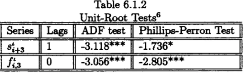
29.99 11

Table 6.1.2 reports the results of the unit root tests. We performed two unit-root types of tests: The Augmented Dickey-Fuller (ADF, Dickeyand Fuller (1979, 1981» and the Phillips-Perron (Phillips and Perron (1988». The results of the latter are specially relevant, since it corrects the test statistic for the presence of heterokedasticity. Regardless of the test type, the results in the table 1 do not support the hypothesis of one unit root for Si+3 and

ft.a·

II

Series Lags

11 Si+3 1

II

fi.3

110

Table 6.1.2 ＱｊｮｩｴＭｾｴ＠ Tests6

ADF test

II

Phillips-Perron Test -3.118*** ｾ＠ -1.736*

II

-3.056***

II

-2.805***

_II

Phillips (1986) pointed out that spurious effects on the t-test distribution can only be caused by the lack of stationarity or ergodicity in the variables. We have showed, however, that spurious effects on the t-test appears as a result of the presence of local persistence in the data. Consequently, even if the data do not support the hypothesis of a unit root, we still need to check whether they support or not the hypothesis of stationarity

(d

= O) against the altemative of local persistence

6The nu.mber of lags only apply to ADF testo The final choice W8S made based on the

t-test of significance of the 1ast first..difference ooefficient. The lag-truncation parameter used in Phillips-Perron test W8S equal to 5, which oorresponds to value suggest by

Newey-West. Since ＸｾＫＳ＠ and

It,3

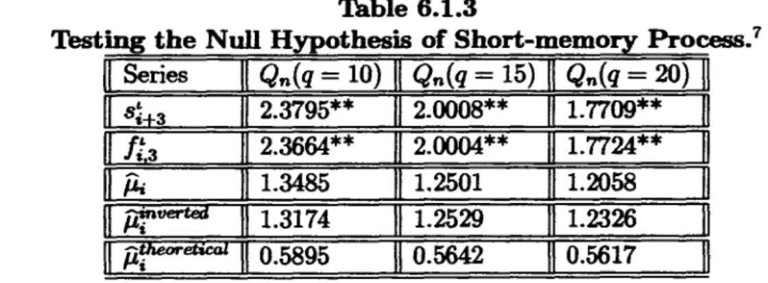
are demeaned processes, we used the non-intercept specification. The symbol (***) indicates rejection of the null at 10%,5% and 1% levei of significance, respectively. The symbol (*) indicates rejection at 10% leveI of significance. The criticaI

Table 6.1.3 presents the results for the test of the null hypothesis of sta-tionarity, which was introduced by this paper in the section 5. It is clear from table 6.1.3 that the test statistic decline monotonically as q increases. However, these series are supposed to be temporally dependent, and such a serial dependence should be taken into account when we estimate the long-run variance. For bandwidth choices q

=

10,15, and 20. We find that the data do not support the null hypothesis of stationarity

(d

=

O)

for

Si+3

and

1:,3'

This result implies that si+3 and

1:,3

may comove if the residual process

is stationary.

On

the other hand, the altemative hypothesis implies that the residual process exhibit local persistence, which means that si+3 and

1t,3

do not comove.

We have used three measures of the residual processo The first measure is the one suggested by the Eq. (6.1.4), that is, one first regresses

Si+3

onto

_1:3

and then calculate the residual

f4.

The second measure,

ílftJel'ted,

is calculated by regressing

1:,3

onto

Si+3'

Finally, the last measure is calculated in line with what is predicted by the underlying theory, that is, ￭ｩｾ･ｴｩ｣ｯｬ＠

=

Si+3

-

1t,3'

Regardless the measure used, one cannot reject the null hypothesis that the residual process exhibit short-memory persistence for all the three suggested values of the truncation parameter. This means that there is co-movement between

It,3

and si+3 and that,in particular, they can co-move with comove-ment vector equal to (1, -l),which corresponds to the theoretical vector. Since li,3 and

Si+3

may statistically have the same mean, the co-movement

between their stochastic components,

1t,3

and

Si+3'

with comovement vector equal to (1, -1), implies to say that the data do support the hypothesis of forward exchange market unbiasedness.

Table 6.1.3

Testing the Null Hypothesis of Short-memory Process.7

Series II Qn(q = 10) II Qn(q = 15) Qn(q = 20) II

Si+3

II 2.3795** 11 2.0008** 1. 7709** I

ft.3

li

2.3664** 2.0004** 1.7724**

íli 111.3485 1.2501 1.2058

I

jlfiJêrtéti 111.3174 1.2529 1.2326

I

II

íiF

êtlêâl II 0.5895 0.5642 0.5617 "

In conclusion, this empirical example seems to illustrate very well the imporlance of the test we have proposed here. In particular, each variable does not have a unit root but still exhibits local persistence. Since local persistence causes spurious effects on the t-statistic, one should not rely on the results based on a t-test. Hence, the residual based test introduced in this paper

fills

in an imporlant gap in econometrics, and enable us to check the validity of the hypothesis of co-movement between two processes with local persistence, even under the presence of simultaneous equation bias.

We now turn to another imporlant puzzle in macroeconomics, which is the validity of the Fisher EHects.

6.2 Testing For Long-Run Fisher Effects.

6.2.1 The Model.

The Fisher hypothesis has been one of the most studied topics in economics. It states that there must exist an one-to-one relationship between nominal interest rate and expected infiation. This relationship is summarized by Eq. (6.2.1) below

ｩｾ＠ = Om

+

.l3mE[7r:']

+

ｵｾ＠

(6.3)

where

E[.]

is the expectation conditional on all information available at time i

E

i

[1If]

= m-period expected inflation rate from time i to i + m,

ｩｾ＠ = m-period nominal interest rate known at time i.

Expected inflation is hardly observed. Instead, one observes the ex-post inflation rate

(6.4)

Consequently, the relationship expressed by Eq (6.2.1) can be rewritten in the following formo

ｩｾ＠ = Om

+

.13m

7r:'

+

ｦｉｾ＠

(6.5)

even under the presence of endogenous regressors, i.e.,

E[7rfl1i]

=I

O. In

order to do so, we will assume the following model:

nf2

-

C-,r

+

1r;

ii

2

- Ci

+

ir

fI -

Ãn1r; +

/ii,

where

Jí,i

=

1(0)

underHo.

(6.6)

where

'Ir[

and

i[

are demeaned versions of the 12-month ex-post infiation and nominal interest rate

(al!

of them are observed monthly). Eqs (6.6), therefore, tells us that future inflation and nominal interest rate can be mod-elled as a deterministic component plus a stochastic termo

6.2.2 Main

Results

The data are showed in the figure ｾＮ＠ The timing of the data is as follows: A January interest rate uses the end-of-January 12-month bill rate data. A January observation of the twe1ve-month inflation rate in the year i is calculated from the January

CPI

data in the year i to the January

CPI

data in the year i

+

1. Figure 2 indicates that inflation as well as interest rate seem to have mean reversion, but it also shows that the mean-reverting speed is pretty low.

Table 6.2.1 contains the estimates of Eq. (6.2.3) for horizons of twelve months by assuming that interest rate and inflation are short-memory pro-cesses. The t-statistic reveals that the null hypothesis

13m

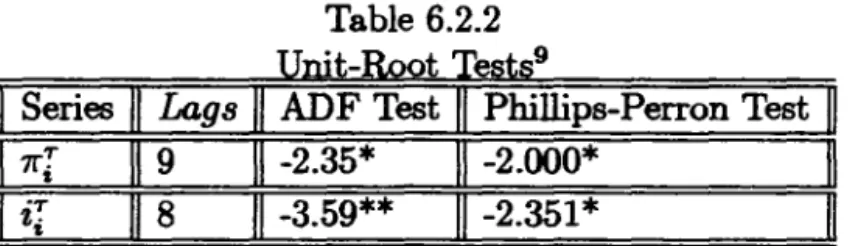
= O cannot be accepted, which would imply that one should accept the hypothesis of Fisher effects. However, inference with t-distributions can be highly misleading if

the variables in the Eq. (6.2.3) contains stochastic trends. The test of a unit root in the series of ex-post inflation and nominal interest rate is presented by table 6.2.2.

8cpI: We have used CPI data-all urbana and non-seasonally adjusted index - collected from Board of Governors of the Federal R.eJerve System, http://www.stJs.frb.orgffrOO/

12 10 8 6

4

!

2

O -2 -4 -6

12-month Demeaned Future Inflantion and Demeaned Nominallntere.t Rate

Oemeaned Future Inflation

Oemeaned Nominalln1erest

RAtA

'\

..

:.

Ｚｾｉ＠

ＺＺｾ＠ ::

,. ...,.

ｾＬＮ＠ :

Table 6.2.1

Estimates

or

the Equation 6.5

(standard

errors in parenthesis)

'm a...m m

'ti = Ckm

+

}Jmlli

+

TJi

One can see that, regardless of the test type, the results in the table 6.2.2 do not support one unit root for demeaned future inflation and demeaned nominal interest rate.

Table 6.2.2 Unit-Root Tests9

11 Series " Lags 11 ADF Test " Phillips-Perron Test 11 11 1[[ II 9 II -2.35* 1\ -2.000* II

" ir "

8 " -3.59** " -2.351* 11

We have showed that spurious eHects on the t-test distribution also ap-pears as a result of the presence of regional persistence in the data. Conse-quently, we must still check whether the data support or not the hypothesis of short-memory persistence, even if they do not support the hypothesis of an unit root.

In the table 6.2.3 We test the null hypothesis that

ir

and

1fT

are sta-tionary (d = O) against local persistence (O

<

d

<

1). Once again, the test statistic declines monotonically as q increases. Since these variables presents temporally dependence, we need to calculate the long-run variance by taking into account such a serial dependence. For q = 5,10 and 15, the results indicate that one cannot accept the null hypothesis that future infiation and nominal interest are stationary processes. Consequently, the results reported in the table 6.2.1 may be highly misleading because local persistence may

9The number or lags only apply to ADF testo The final choice was IDade based on the t-test or significance or the last first-djffereooe coeffi.cient. The lag-truncation parameter

used in Phillips-Perron test was equal to 5, which corresponds to value suggest by Newey-West. Since 7r[ and i[ are demeaned processes, we used the non-intercept specification. The symbol (**) indicates rejection or null at 5% and 1% levei. The symbol (*) indicates rejection at 5% leveI of significance. The criticaI values are, -1.94, and -2.57 for 5% and

generate spurious effects on the t-test. Although the hypothesis of Fisher effect cannot be tested by using the t-test, one still can verify the validity of such hypothesis by investigating whether the residual process exhibit short-memory persistence (stationarity) or noto Notice, however, that

1[J

seems to be less persistent than

iJ,

since we can no longer reject the null hypothesis at

1%

leveI of signif1cance for ff[ when q =

15,

whereas we can still do so for

ir

when q

=

15.

Consequently, one expects that the Fisher hypothesis will never be accepted because

it

and ff[ display different levels of local persis-tence, which implies that the residual process will also display local persistent behavior. In order to see the validity of this conjecture, we have chosen two measures of the residual processo The first one is calculated by using the Eq.

(6.2.6),

and the second one,

iir

verted_{, is calculated by regressing ff[ onto}

ir.

Regardless the measure of residual process used, table

6.2.3

indicates that the data do not support the hypothesis of stationarity in the residual processo Consequent1y, unlike what is concluded when we use the t-test, we cannot accept the null hypothesis of long-run Fisher effects.

Table 6.2.3

Co-movement Between Inflation and Nominal Interest Rate.lO

II

Variable

II

Qn

(q

=

5) I1

Qn

(q

=

10) 11

Qn

(q

=

15) I1

I1 1[[

I1 2.34**

111.76**

111.48*

11

'T

ｾｩ＠

2.90**

2.18**

1.83**

Jl.i

3.04**

2.30**

1.95**

11

iir

verted

_{11 2.36**}

_111.78**

_111.524**

11

7. Conclusion

We proved that when one regresses a process with local persistence onto another one that also exhibit local persistence, then spurious effects on the t-statistic will appear. We, therefore, derived a residual based test, through which the null hypothesis of co-movement between two processes with local persistence can be tested consistently, even under the presence of a endoge-nous regressor. Asymptotic distributions of this test are derived under both the null hypothesis and the alternative hypothesis of local persistence. The lOThe symbol (**) indicates that the oull is rejected at the 5% and 1% levei of

signifi-caore.

limiting distribution under the null is a function of Brownian motions, involv-ing the ｾ｣｡ｬｬ･､＠ Brownian bridges. The limiting distribution under the null

is also free of nuisance parameters, meaning that we do not need to employ fully-modified estimation. Tables of criticaI values are provided based. on the asymptotic null distributions. The test statistic diverges under

H1'

and the divergence rate depends on the bandwidth parameter. A Monte Carlo experiment was conducted to examine the finite sample performance of the teso In particular, finite sample size and power were studied. Finally, this test was employed to verify the validity of two important hypothesis in eco-nomics: the forward exchange rate unbiasedness and the Fisher hypothesis. The data used in this paper support the null hypothesis of forward exchange rate unbiasedness but do not support the Fisher hypothesis.

APPENDIX: PROOFS

Proof of Theorem 1.

(a)

(fi

-

(3)

=

Op(n

d/

2- I/2).

Proof: Following Phillips et al(2001), we know that

M m 1

(i)

it

k"fI

n!2

ｾ＠

(Xk,t)2

--t

E(l H:,c(r)2dr).

Using the same procedure, it is easy to show that:

M m

(ii)

Tu

L

n!2

L (Xk,tUk,t)

=? Normal

DistrilJUtian

=

Op(l).

k=I

t=1

Therefore

n

1/

2-

d/

2

_(fi

-

(3)

=

Op(l),

which implies that

(P -

(3)

= Op(n

d

/

2-

1/

2).

(b)

ｾ＠

=

Lk

Jm

ｌｴｪｌｾＬｴ＠

= Op(m)

--t 00.

M

Proof: Noticethat 1.. _m ｌｴｊｩＬｾｴ＠ _,

= Op(m).

Therefore,

Lk MIm LtJi,L =

_,

M

I L Op(m)

_k=I =

Op(m)

(c)

Vãr(P) = ｾＨｌｫｌｴｾＬｴＩＭｉ＠ =

Op(n-

1).

Proof: We have already proved that ｾ＠ =

Op(m).

Notice n-om result (i)

m M

that

L (Xk,t)2

= Op(m2).

Hence,

L Op(m2) = Op(Mm2).

This

implies that

t=1

k=I

-(f.i)

Op(m) O

((M

)-1) O ( -1)

var fJ

=

O,,{Mm2)

=

p m

=

p n .

fi

(d)

t-p

=

Op(n2)

and therefore

tfi

--t 00.

From (b), ＨｾＭ

(3)

=

Op(n

d

/

2- 1/2).

From (c), Ｈｖ｡ｲＨｾﾻＱＯＲ＠

=

Op(n-1/2).

Therefore

o

(nd/ 2- 1/ 2 )

ｴ ｾ＠ - p -

o

(nd/ 2)

(3 -

Op(n-1/2)

-

p .

(e)

R

2 _{-+ O.}

Given that

Xk,t

and

Yk,t

are two stochastic block local to unity processes

M m

ｾ＠

I:

ｉＺｾＬｴ＠ M m

with mean zero, then

R 2

= ｛ＱｬｾＱｴＺＱ＠ . Notice that

I: I:

ｘｾＬｴ＠ =

Op(Mm2)

ｾ＠ ｾｾ＠ k=lt=1 L..J L..J Io,t

10=1 t=1

M m

M m

I:

ｉＺｾＬｴ＠

and

I: I:

ｾＬｴ＠ =

Op(Mm2).

Therefore ｾＱｴ］［ＬＬｴ＠

k=1t=1 ｾ＠ ｾ＠ 2

L..J L..J 1IIo,t

10=1 t=1

fi2

=

ap(l),

it follows that

R

2 _{-+ O.}

Proof of Theorem

2. By definition

Maz

1

tJ

11

tJ ｾ＠ 1 n ｾ＠

I

Qn = l<tJ<n ｔｮｾ＠

;;

ｾ＠ Jl.i - ｾ＠

.I:

/Ji

- - ,. ｾＱ＠ ｾＱ＠

_ Maz 1 1

ｾｬ＠ ｾ＠

.l!!!:l(

1

ｾ＠ ｾ＠

)1

- O<r<l _{- - , .} ｾ＠ n1 /2 .L..J Jl.i - n n1/2.L..J Jl.i

ｾＱ＠ ｾＱ＠

=

Op(l)

and, given that

1 [nrJ

We have already showed that

vfii

ｾ＠

íli

=>

ｂｾＨｲＩ＠ = ｷｾｗｾＨｲＩＬ＠ with O

<

d

<

l.

Thus, by the fact that ｾ＠ -+ r and the continuous mapping theorem,

[nrl n 1

ｯｾｲｾｬ＠

t

n;72

ｾ＠

íli

-

ｾＨｮＺＯＲ＠

I1

Pi)

=>

ｏｾｬ＠

ｉｗｾＨｲＩ＠

-

ｲｗｾＨｬＩｬﾷ＠

Where ｗｾＨｲＩ＠ - ｲｗｾＨｬＩ＠ is a standard Brownian bridge.

Proof of Theorem

3.

Theorem

3 : H

YI

and

xi

are two stochastic block local to unity processes

with d.rift and O

<

d

<

1, then under Ho and assumption 1, the following

wi11 hold as (m, M -+ OO)Beq

Qn =

ｬｾｾｮ＠

**

IE

Pi

-;;

Êí

ílil :::}

ＰＤｾＱ＠

ｉｗｾＨｲＩ＠

-

ｲｗｾＨｬＩＱ＠

where the residual series

Pi

is collected from the regression 3.

In order to derive a proof for the theorem 3 above, we need to derive first the asymptotic behavior of ｾＱＱ＠ and ｾｺＮ＠ Following Phillips et al (2001), let Dn be the standardized matrix so that

D;

1 _{T (nr)}

_=>

_{T( r) = (1, r)', the limiting}

(i)

n1/2-dn

(in

-

(n ) =

ＨｾＩ＠

[1

ｾ＠ ｄＭＱｔＮｔｾｄＭＱ｝ＭＱ＠

ｾ＠

D-1T. Yi

n TY TY -c n 4- n ' , n 4- n ' ! + d

, ' n 2

ｾ＠

[IT(r)T(r)'drr [IT(r)dTJl'(r)]

where

UY(r)

:= ｂｍＨｷｾＩ＠

-1 ｾ＠

(ii)

n1/2- dDn( épx- C(Jx)

=

｛ｾｾｄ［［ｉｔｩｔｾｄ［［ｉ｝＠

ｾｄ［［ｉｔｩ＠

ｾＺ､＠

, ' n2

ｾ＠

(!J

[IT(r)T(r)'df

[IT(r)dU"(r)]

where

UX(r)

:= ｂｍＨｷｾＩ＠

Notice that the scaling matrix above

n1/2- d Dn

=

.jiim-1 Dn

=

diag[ni m - 1,

ni

MJ.

This matrix indicates that consistent estimation of intercept and of slope of linear trend is possible when c

<

O provided that

v'fim-

1 _{--+ 00 or,}

equiva-lently, :: --+ 00.

Now, remember that

ｾ＠ T ｾｔ＠ Ｈｾ＠

)'T

Yi

= Yi

-

C(Jy

i

= Yi

-

C(Jy

-

C(Jy

i

and

Xi

=

xi

-

ép'x

Ti

=

xi

-

(épz

-

C(Jz)'T

i

Therefore, one can show that

[nr] [nr] 1 [nr]

(1)

i+tl.I:

Xi

=

i+tl

ｾ＠

Xi

-

[n

2 -

d Dn(épz

-

C(Jz)]'

.L

n-1 D;;IT

i

n 1=1 n 1=1 1=1

ｾ＠

Normal Distribution-

[j

T(

8

)T(

8)' ds

r

[j

T(

8

)dU"(

8)

r

j

T,(

8 )ds =

Op(l)

Recall that the residual,

'A,

is estimated from regression

fA -

fixi

=

'A,

M m ti

_ I: I:(z",tU",t)

L

(z,íii) where f3

=

ｉ］ｾｴ］ＡＮ＠

=

］［ｾｦＭＱ＠

-I: -I:(i'",t)2 I:(z.)2

1=1 t=l i=1

Thus, from Phillips et ali (2001), one can show that:

M m

_ *'

L

ｾ＠

L

(i'",t;;",t)

(lI)

../Mm(/3

- /3)

=

"';,,1 t=!.

=>

N(O, 1)

ｾ＠

L

ｾ＠ I:(z",t)2

"=1 t=1

This implies that

fi

is a ｮｩＫｾ＠ -consistent estimator of

/3.

One can also show that limit distribution of

../Mm(fi-

/3)

is the same as that of

Now we use (I)

+

(lI) to show that

1 [nr] 1 [nr]

!+! _

[nr]

-

_.;n

L

iii

= -

L

I-'i - ｾＨｦＳ＠

-

13)

/+<1

L

Xi .

i=l

.;n

i=l n -r n i=l

Since O

<

d

<

1, it turns out that the second term will vanish, implying that

1 [nr] 1 [nr]

-

_.;n

L

ii.

= -

L

/L.

+

Op(1)

i=l

vIn

i=1

Thus,

ｾ＠ ｛ｾ｝＠

ii.

=>

B,,(r)

=

w"W,,(r),

where

'fí.i

isnowestimatedfromregression

yni=1

2, i.e.,

'fí.i

=

fi.

-

f3x •.

Lastly, theorem 2 can be used to prove that

Qn

=

ｉｾｾｮ＠

7,;*

IE'fí.i - ;;

E

'fí.il

=>

ｾｓＺｾｬ＠

IW,,(r)

-

rW,,(1)1·

Proof of Theorem 4.

Theorem 4. Under the alternative hypothesis that I-'i display local per-sistence and assuming that the bandwidth parameter q

=

Op(n

d

), then the

following will hold as

(m,

M ｾ＠

oo)seq.

1 [nr]

vnf

(i)

1 -

L

j4 = Op( nd).

'!Dp.

Vn

i=l q

(ii) Qn ｾ＠ 00, indicating that, under the alternative hypothesis, the test

statistic will reject the null with probabilily one

The result above is valid no matter whether the dependent and indepen-dent variables are stochastic block local to unity processes with linear trend or noto

Proof:

For the estimation of

w",

we consider the estimator

iiP

=

t

(1 -

1M ):y(h)

"h=-q q

n-Ihl ｾ＠

where :y(h) = 1.

L

j4íii+h, j4 = Yi -

f3x •.

It is well known that under

n i=I

HI' :y(h) =

Op(m)

and consequently

w!

=

Op(mq). Under HI, it can verified 1 [nr]

that ｾ＠

L

i4

=

Op(m). yn i=l

Thus, 1 [nr]

t

ｾ＠ ｾ＠

i4

=

Op(

ｾＩ＠ =

Op(

ｾＩＮ＠ Given that q

=

Op(n

d), we get a

p. y n 1=1

v...

V

q

References

[1] Chan, N.H., and Wei, C. Z. (1987). "Asymptotic Inference for NearIy Nonstationary AR(I) Processes, Annals of Statistics, 15, 1050-1063. [2] Dickey, D.A., Fuller, W.A.(1979).Distribution ofthe estimators for

auto-regressive time series with a unit root. Journal of the American Statis-tical Association, 74 (366), 427-43l.

[3] Dickey, D.A., Fuller, W. A. (1981). Likelihood Ratio Statistics for Auto-regressive TIlDe Series with a Unit Root. Econometrica 49 (4), 1057-1072.

[4] Elliot, G. (1995). On the Robustness of Cointegration Methods When Regressors Almost have Unit Roots, UCSD Discussion Paper 95-98. [5] Feller, W. (1951): "The Asymptotic Distribution of the Range of Sums

of Independent Random VariabIes," Annals of Mathematical Statistics, 22,427-432.

[6] Kwiatkowski, D., Phillips, P. C., Schmidt, P., and Shin, Y. (1992). Test-ing the null hypothesis of stationarity against the alterna tive of a unit root: how sure are we that economic time series have a unit root? Jour-nal of Econometrics. 54, 159-78.

[7] Phillips, P.C.B. (1986): "Understanding Spurious Regression in Econo-metrics," Journal of Econometrics 33, 311-340.

[8] , Perron, P. (1988). Testing for a unit root in time series re-gression. Biometrika 75, 335-346.

[9] , (1998): Econometric Analysis of Fisher's Equation. Depart-ment of Economics, Yale University.

[10] , and Hansen, B.E. (1990): "Statistical Inference with 1(1) Pro-cess" Review of Economic Studies, 53, 473-496.

[11] , Moon, H.R., and Xiao, Z. (2001): How To Estimate Autore-gressive Roots Near Unity. Working paper, Yale University.

Non-[13] , Solo, V., (1992): "Asymptotics for Linear Processes" , Annals of Statistics 20, 971-100l.

[14] Protter, P. (1990), Stochastic Integration and Differential Equation, Springer, New York.

[15] Xiao, Z. (1999): "A Residual Based Test for the Null Hypothesis of Cointegration," Economics Letters, 64, 133-141.

FUNDAÇÃO GETULIO VARGAS BIBLIOTECA

ESTE VOLUME DEVE SER DEVOLVIDO À BIBLIOTECA NA ÚLTIMA DATA MARCADA

35

B\6L10TECA MAIõtO ｈｅｎｒｉｾｕｉ＠ S1MONSEN

G

-'>.

ｾＩ［＠ I ',...

-f

_ _ _ J ｾＭｾＮ＠

BIBLIOTECA MARIO HENRIQUE ｾｉｍｏｎｓｅｎ＠

N.Cham. PIEPGE SPE L 732c

Autor: Lima, Luiz Renato