Extending Ripley's K-Function to Quantify Aggregation in 2-D Grayscale Images.

Extending Ripley

_’

s K-Function to Quantify

Aggregation in 2-D Grayscale Images

Mohamed Amgad1,2*, Anri Itoh1, Marco Man Kin Tsui1*

1Okinawa Institute of Science and Technology (OIST) Graduate University, Okinawa, Japan,2Faculty of Medicine, Cairo University, Cairo, Egypt

*mohamed-amgad1@hotmail.com(MA);marco.tsui@oist.jp(MMKT)

Abstract

In this work, we describe the extension of Ripley’s K-function to allow for overlapping events at very high event densities. We show that problematic edge effects introduce sig-nificant bias to the function at very high densities and small radii, and propose a simple cor-rection method that successfully restores the function’s centralization. Using simulations of homogeneous Poisson distributions of events, as well as simulations of event clustering under different conditions, we investigate various aspects of the function, including its shape-dependence and correspondence between true cluster radius and radius at which the K-function is maximized. Furthermore, we validate the utility of the function in quantify-ing clusterquantify-ing in 2-D grayscale images usquantify-ing three modalities: (i) Simulations of particle clustering; (ii) Experimental co-expression of soluble and diffuse protein at varying ratios; (iii) Quantifying chromatin clustering in the nuclei ofwtandcrwn1 crwn2mutant Arabidop-sisplant cells, using a previously-published image dataset. Overall, our work shows that Ripley’s K-function is a valid abstract statistical measure whose utility extends beyond the quantification of clustering of non-overlapping events. Potential benefits of this work include the quantification of protein and chromatin aggregation in fluorescent microscopic images. Furthermore, this function has the potential to become one of various abstract tex-ture descriptors that are utilized in computer-assisted diagnostics in anatomic pathology and diagnostic radiology.

Introduction

Spatial point analysis, the analysis of dispersion and clustering of events, has been well-studied and heavily utilized in many fields [1,2]. One of the earliest attempts at providing a solid math-ematical foundation to quantify“significant”clustering or dispersion was that of Clark and Evans in 1954, which relied on the“average distance to the nearest neighbor”[3]. However, the problem with Clark’s method is that it does not quantify clustering at different scales, unlike other methods that have been later devised to address this issue.

Nowadays, Ripley’s K-function, developed in 1977, is considered to be the“golden stan-dard”in spatial point analysis [4]. Since its original development, Ripley’s K-function has been OPEN ACCESS

Citation:Amgad M, Itoh A, Tsui MMK (2015) Extending Ripley’s K-Function to Quantify Aggregation in 2-D Grayscale Images. PLoS ONE 10 (12): e0144404. doi:10.1371/journal.pone.0144404

Editor:Ina Maja Vorberg, Deutsches Zentrum für Neurodegenerative Erkrankungen e.V., GERMANY

Received:November 22, 2014

Accepted:November 18, 2015

Published:December 4, 2015

Copyright:© 2015 Amgad et al. This is an open access article distributed under the terms of the

Creative Commons Attribution License, which permits unrestricted use, distribution, and reproduction in any medium, provided the original author and source are credited.

Data Availability Statement:All relevant data are within the paper and its Supporting Information files.

Funding:The authors have no support or funding to report.

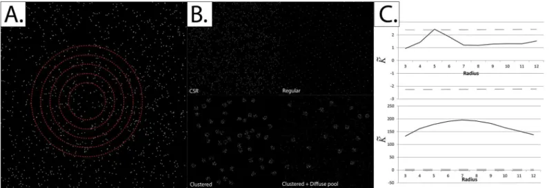
extensively used in a very large spectrum of applications, including geography, epidemiology, economics and biomedical research [1,2,5–8]. The concept behind Ripley’s K-function is rather simple; it is the average number of events (particles) located within a predefined radius of any typical event, normalized for the event intensity (density) over the same field of view. Ripley’s K-function compares the distribution of events in a given field of view to Complete Spatial Randomness (CSR), otherwise known as a“homogeneous Poisson process”. At CSR, the loca-tions of events are completely random; not regular but random (Fig 1).

Previous attempts to integrate Ripley’s K-function into image processing include its utiliza-tion in concrete (segmentautiliza-tion-based) statistics [9,10]. In this paper, we test and optimize the use of Ripley’s K-function as an abstract index of clustering, to allow for event overlap at very high densities. As will be described later, problematic edge effects become of particular rele-vance at very high densities, and previously-reported patterns linking the radius at which the K-function is maximized with the underlying cluster radius break down. But why would it be useful to extend Ripley’s K-function to allow for event overlap? Our main motivation was to develop an image processing approach to quantifying protein aggregation in fluorescent micro-scopic images.

While the quantification of higher order protein homo-oligomerization and aggregation propensityin-vitrohas been thoroughly developed over many decades of protein biochemistry research, the quantification ofin-vivooligomerization or aggregation has received relatively less attention. Over the past few years, however, the importance ofin-situcharacterization of protein solubility and aggregation became increasingly clear [11]. This paradigm shift has been caused by a number of developments in protein research including:a)a better understanding of the role played by complex intra-cellular environments in altering reaction equilibria and causing a disparity betweenin-vitroandin-vivoassays [12,13],b)a wealth of evidence outlin-ing the crucial involvement of protein aggregation in a multitude of diseases, includoutlin-ing Alzhei-mer's disease, Huntington's disease, Amyotrophic Lateral Sclerosis (ALS), Parkinson's disease and Prion disease [14],c)an increasingly widening scope of protein aggregation research to include emerging fields such as ageing research [15,16], andd)the realization that bacterial inclusion bodies (IB's) may be used as sources of active recombinant proteins [17] as well as a model system for amyloid aggregation studies [18].

One of the most problematic issues that arise when trying to quantifyin-vivoaggregation of proteins is the interference caused by the soluble pool of proteins with accurate and specific identification and characterization of aggregates. Several experimental approaches have been devised to overcome this limitation, and fall into four broad categories, reviewed in a recent commentary by Amiet al[11]: Genetically-encoded fusion tags such as GFP or tetra-Cys tags; Conformation-sensitive dyes such as Thioflavin-S; Direct spectroscopic methods such as Nuclear Magnetic Resonance (NMR); Aggregation-sensitive reporters. The majority of these experimental approaches rely on parameters that can differentiate between soluble an aggre-gated forms of proteins.

Oftentimes, proteinsin their native stateoligomerize and form cytoplasmic puncta which may or may not be of regular sizes and shapes, and which may constitute only a fraction of the amount of protein in the cell, the rest being in diffuse (soluble) form [21–23]. In such cases, studies of protein supramolecular complexes or aggregates traditionally involvedin-vitro bio-chemical methods such as chromatographic and centrifugation assays to separate aggregates from soluble protein pools. The problem, however, is that these biochemical techniques are often prone toin-vitroartifacts.

Generally speaking, there are two broad categories of calculations that can be applied to two-dimensional fluorescence microscopic images: "concrete" (segmentation-based) statistics and "abstract" (e.g. texture) statistics [24]. Concrete statistics try to separate out objects from background (segmentation), allowing further calculations to be performed on the objects such as total intensity, volume, localization and so on. Depending on the context, the most suitable segmentation techniques may vary considerably [25]. We faced some difficulty when we tried to quantify the effect of various mutations on the incorporation of a protein,Cubitus interrup-tus(Ci), into cytoplasmic puncta using confocal fluorescence microscopy. The differentiation between punctate and diffuse protein forms in our case was often tricky due to the following factors:a)the presence of a soluble pool introduces high background, reducing signal-to-back-ground ratio;b)the amount of soluble protein is variant in different regions, causing high vari-ability in background intensity;c)clumping of aggregates introduces further ambiguity into the image segmentation process. Besides, the highly heterogeneous nature of the aggregates prevents filtering based on a common morphology, as would have been possible for tube-like [26] or sheet-like [27] structures, for example.

Can an abstract statistical metric be used to quantify protein aggregation? Because of the low signal-to-background ratio and the inherent variability in background in images of protein aggregation studies, isolating aggregates reliably using concrete statistical measures (i.e. seg-mentation) may sometimes be very difficult. The golden standard, of course, would be to devise better experimental methods that enable the reliable separation of proteins in the soluble and

Fig 1. The concept behind Ripley’s K-function.Panel A: Ripley’s K-function is defined as the average number of events within a predefined radius of any event, normalized for the event intensity (density) over the whole field of view. A set of radii is typically used to quantify the scale at which clustering (or dispersion) of events occurs (red circles).Panel B: Events within a given field of view could be distributed in many forms, including Complete Spatial Randomness (CSR), regularity and clustering (with or without a diffuse pool).Panel C:_K~_{plots for two of the event distributions in Panel B: CSR (upper) and}

aggregated pool. However, were this unavailable, it may be necessary to use an abstract metric to quantify aggregation. Many abstract image metrics exist, including simple histogram-based metrics such as mean, variance, skewness and kurtosis, and Haralick Gray Level Colocalization Matrix (GLCM) texture descriptors [24,28]. Besides, a number of user-friendly machine learn-ing programs have been developed, most notably CellProfiler and CellProfiler Analyst [29,30], that allow automatic identification of features of interest after initial training by the program user. As we will describe later, we demonstrate the validity of our extension of Ripley’s K-func-tion as a theory-driven abstract index in quantifying protein aggregaK-func-tion using simulated and experimental ground-truth controls. In addition, we argue for the generalizability of our approach by performing a proof-of-concept analysis on a previously-published dataset, in order to validate its use in chromatin condensation quantification as well.

Materials and Methods

1. Software used and data availability

All simulations and image processing codes were written and maintained in MATLAB (Ver-sion R2015a, The Mathworks Inc., USA). Preprocessing of protein aggregation images was done using ImageJ 1.49v and CellProfiler 2.1.1 [29,31]. The dataset and codes used for K-func-tion calculaK-func-tion and validaK-func-tion are available in the supplementary materials (S1andS2Files).

2. Mathematical development

2a. The original K-function. Ripley’s K is given by the equation: Kðr;nÞ ¼

1

lEðnumber of events within radiusrof the}typical}eventÞ ð1Þ

WhereEis the expectation (i.e.“average”) number of events within radiusr,nis the total num-ber of events within the study area andλ_{is the intensity (density) of events, such that} l_¼ n

jOj

and |O| is the area of the study region (the entirefield, including all potential event locations). Hence:

Kðr;nÞ ¼jOj

n

1

n 1

Xn

i¼1

Xn

x6¼y

IrðdxyÞ ð2Þ

Wheredxyis the distance between event locationsxandyandIris an indicator function that

has a value of 1 if the distance between locationsxandyis less or equal tor. That is,

IrðdxyÞ ¼

1 if dxyr

0 otherwise (

the central event. One of the best and most widely accepted methods to correct for this bias was proposed by Besag [32]. Instead of correcting for events at each distance from the central event separately, Besag’s correction corrects for all events at once. That is, the overall number of events within a particular radius is divided by the proportion of the area of a circle of the same radius (centered on the central event) that is included within the field of view. For these reasons, we used Besag’s edge correction for all experiments in this paper.

Therefore,

Kðr;nÞ ¼ jOj nðn 1_Þ

Xn

i¼1

p_r2

Axr

Xn

x6¼y

IrðdxyÞ ð3Þ

Axris the area of the portion of circleb(x,r), centered on positionxand having a radiusr,

that lies within the study region. Besag’s edge correction term is given by the equation: Axr ¼bðx;rÞ \ jOj

Because Ripley’s K-function normalizes for the event density, its expectation at CSR is sim-ply the area a circle of the same radius as that used to calculate the function. One problem with the original K-function is that it is not centered on zero, nor is it normalized to have a unit vari-ance. While there are multiple versions of the K-function (including the L- and the H- func-tions [32,33]), we used the version proposed recently by Lagacheet al[34], which also has a unit variance, and has the following equation:

~

Kðr;nÞ ¼ Kðr;nÞ

p_r2

ffiffiffiffiffiffiffiffiffiffiffiffiffiffiffiffiffiffiffiffiffiffiffiffiffi varfKðr;nÞg

p ð4Þ

Once the K-function of a particular field of view is obtained, it is compared to the upper and lower limits (typically, the 1stand 99thquantiles) of what its value would be at CSR. The theo-retical determination of these“critical quantiles”proved to be especially difficult due to edge effects, and even though multiple attempts existed in the past, extensive Monte-Carlo simula-tions remained to be the only reliable method for critical quantile determination. It wasn’t until recently that Lagache and colleagues provided the first solid theoretical foundation for critical quantile determination, based on the Cornish-Fisher expansion [34]. As can be seen in

Fig 1C, at CSR_K~_{lies within the bounds of the theoretically-determined critical quantiles, while}

it lies outside these bounds when the events are clustered.

2b. Extension to allow for event overlap. Our extension of Ripley’s K-function is as fol-lows. We imagined each intensity unit to be one particle such that, in an 8-bit grayscale image, the saturation limit is 28−1 = 255 particles per pixel. The number of particles around any parti-cle within the same pixel =Px−1, wherePxis the intensity at pixelx. The number of particles

around any particle in surrounding pixels within a circle of radiusr=X

Np

x6¼y

IrðdxyÞ, whereNpis

the total number of pixels in thefield of view andIrðdxyÞ ¼

Py if dxyr

0 _otherwise (

.

Hence, the number of particles within radiusraround each particle at pixelx=

Px 1þ

XNp

x6¼y

IrðdxyÞ ð5Þ

r=

p_r2

Axr

Px Px 1þ

X

Np

x6¼y

IrðdxyÞ

!

ð6Þ

Finally summing up over the whole field of view and normalizing to obtain K,

Kðr;nÞ ¼ jOj

nðn 1_Þ X

Np

i¼1

p_r2

Axr

Px Px 1þ

X

Np

x6¼y

IrðdxyÞ

!

ð7Þ

WhereNpis the total number of pixels andnis the total intensity (i.e. total number of particles)

over the wholefield of view.

2c. Different implementations of Besag’s edge correction term. To test the validity of our extension of Ripley’s K-function to grayscale (non-binary) fields of view, we devised the following validation workflow (illustrated inFig 2).

We generated synthetic fields of view measuring 256 x 256 pixels and assigned particles at various densities to these pixels in a random manner, in order to create a homogenous Poisson distribution (CSR). The densities were exponentially increased and the K-function calculated at four different radii. In order to keep our method suitable for practical applications, particu-larly the quantitative ranking of mutant constructs in order of increasing protein aggregation, we used small-to-medium radii for K-function calculation. Two implementations of Besag’s edge correction term were tested, described by the following equations:

Method I:_{EdgeCorrection¼} pr

2

bðx;_rÞ \ j_Oj

Method II:_{EdgeCorrection¼} bðx;rÞ bðx;_rÞ \ j_Oj

Both edge correction methods were applied to“border pixels”, where a border pixel is defined as any pixel located at a distance less thanrfrom the margin of the field of view. Note that the areab(x,r) is actually less thanπr2due to pixilation effects. As we will discuss in the results section, the two methods fail to maintain centralization of the K-function at high densi-ties, and a simple adaptation where method I was applied to all pixels (not just border pixels) was needed.

3. Validation using simulations

3a. Testing shape-dependence of the K-function. In order to adapt Ripley’s K-function for practical applications, zero pixels were ignored during edge correction, such that Regions of Interest (ROI’s) could be thresholded, with the background given a value of zero, before K-function calculation. Circular decimations, with a radius of 20 pixels, were randomly-scattered across a field of view with a minimum offset of one pixel. After the positions of decimations were determined, events were randomly distributed across all the other locations within the 256 x 256 pixel square field of view.

Signal-to-Background ratio (SBR) constant. (ii) increasing the SBR (effectively increasing the contrast) while keeping the number of aggregates constant.

Simulated 256 x 256 pixel fields of view were used in this experiment, with randomly-located circular clusters (aggregates) having a radius of 8 pixels. The signal was added to the background. In other words, pixels belonging to the aggregates had a value equal to the signal plus the background [35].

After particles were distributed across the field of view, the resulting image was convolved with a Gaussian blur filter having a diameter of 3 pixels and a sigma of 1 pixel, and Poisson noise was generated at high and low Signal-to-Noise ratios (SNR’s), simulating the Point Spread Function (PSF) and noise of a confocal microscope [36,37]. Poisson noise, being the main form of degradation occurring in confocal microscopy [35], was added by applying a Poisson noise generator to each pixel independently, with a lambda equal to the intensity of the pixel of interest [38].K~was calculated for each image at a radius (rk) ranging between 2

and 15 pixels.

3c. Characterizing aggregates. Kiskowskiet alreported that a variable degree of corre-spondence existed between the radius at which Ripley’s K-function was maximized (½_K~

maxŠ)

and the true aggregate radius (ragg) [39]. They showed, using simulations of circular clusters of

particles, that½_K~

maxŠranges between raggand 2ragg, depending on the separation distance

between aggregates, as well as the presence of a diffuse (non-aggregated) pool of particles. We tested whether this still held true when particle overlap was allowed using the following method. Simulated 256 x 256 pixelfields of view were generated, with randomly-located circu-lar clusters (aggregates) having a radius ranging between 2 and 10 pixels._K~_{was calculated for}

each image at a radius (rk) ranging between 1 and 35 pixels.

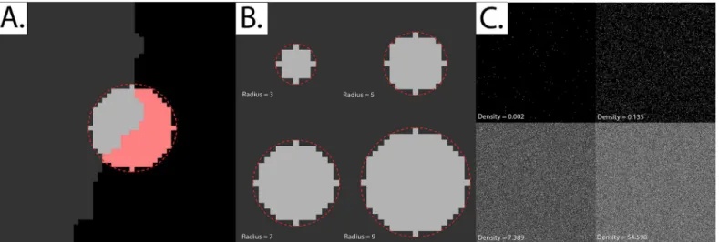
Fig 2. Approaching problematic edge effects at non-binary fields of view and small radii.Panel A: Three implementations of Besag’s edge correction term were tested. Note that the black region (black pixels) are considered to be outside the study region (i.e. the border between the grey and black area represents the edge of the study region), The implementations are as follows: i) Dividing the total number of pixels, located within a pre-defined radius from a given border pixel (light-gray area), by the total area of an ideal circle (area enclosed by the dotted red line). ii) Same as implementation i, but dividing by the total area of a non-ideal/pixelated circle (light-gray plus pink regions). iii) Same as implementation i, but applied for all pixels within the field of view. Hence, even for non-border pixels, the edge correction term would be obtained by dividing the area of the pixelated circle by the area of a perfect circle of the same radius.Panel B: The difference between an“ideal”circle and its pixelated counterpart at the four radii tested in this paper.Panel C: Complete Spatial Randomness (CSR) at a selected number of event densities (intensities). Each field of view measures 256 x 256 pixels. The image intensities were re-scaled for display purposes; the simulations used in Ripley’s K-function validation were set such that one intensity unit is akin to one event, at a saturation limit of 255 events per pixel (8-bit grayscale images).

In addition, we illustrated the use of other, less speculative, techniques in characterizing aggregates. Two well-known methodologies may be used once the“abstract”measure of clus-tering (Ripley’s K-function) has been calculated: segmentation and granulometry. We gener-ated 10 sets of 30 synthetic images, each containing four sets of 20 randomly-locgener-ated

aggregates having radii of 2, 4, 6 and 8 pixels. After particles were distributed across the field of view, the resulting image was convolved with a Gaussian blur filter and Poisson noise was added in the same manner described earlier.

Segmentation of the original images was achieved by passing the synthetic images through an imageJ pipeline consisting of the“Subtract Background”command [40], Auto-thresholding using the“MaxEntropy”method [41], followed by a“Close”operation with edge padding [42]. The granulometric profile was obtained by repeatedly opening the image using progressively larger radii and obtaining the pixel value sum of the resulting image [43,44].

We employed the bivariate similarity index described by Dimaet alto illustrate the compar-ative accuracy and specificity of the two approaches described [45]. The bivariate similarity index, which is itself an extension of the widely used Jaccard Similary Index [46], relies on two measures: TET and TEE, given by the following equations:

TET¼ jT\Ej

jTj where 0TET1

TEE¼ jT\Ej

jEj where 0TEE1

Where T represents the number of non-zero pixels in the ground“Truth”mask, E represents the number of pixels in the“Estimate”mask, andT\Eis the number of pixels that are common to both the Truth and Estimate masks. Note that where there were no non-zero pixels in the Estimate mask, TEE was given a value of one [45].

4. Experimental validation

4a. Quantifying protein aggregation. To further test the validity of our approach, we devised the following experimental setup. We created five constructs containing cells that have been co-transfected with two proteins, Ci and eGFP, which possess different intracellular local-ization behaviors. Ci (Cubitus interruptus) is the main transcription factor in the hedgehog sig-naling pathway. Ci generally exists in two forms in the cytoplasm: diffuse form and aggregated in large protein complexes with other signaling molecules such as Cos2, fused and su(fu) [23,47]. Complexed/aggregated Ci is readily sedimentable by ultracentrifugation [48], and has been shown to dimerize under certain conditions [49]. We found that forced constitutive dimerization of Ci, by replacing its first 440 amino acids with the dimerization domain of CGN4 (GCN4-Ci), results in a predominantly-punctate Ci distribution that appears mainly in the pellet fraction upon ultracentrifugation.

Co-transfection: Clone 8 cell lines [50] were obtained from (and maintained in accordance with) Indiana University's Drosophila Genomics Resource Center. The cells, which were pas-saged every three days, were cultured in T-25 flasks (Corning) using Complete M3 medium (Shields and Sang M3 insect medium Sigma S3652 with 2% FBS (Fetal Bovine Serum, Perbio Science), 100 units/ml penicillin G, 100 mg/ml streptomycin sulphate, 0.125 IU/ml insulin and 2.5% fly extract). Twenty-four hours before transfection, the cells were seeded onto 12-well plates at a density of 0.5x106cells per well. Afterwards, transfection with various amount of DNA was carried out using Effectene transfection reagent (QIAGEN) according to the manu-facturer's protocol. All ROI's shown in this paper are from cells that express the following 3xHemagglutinin (HA) -tagged constructs: (i) GCN4-Ci and (ii) eGFP. The amount of DNA used for each of the five constructs is as follows:

Construct 1–GCN4-Ci: 400ng, eGFP: 0ng; Construct 2–GCN4-Ci: 400ng, eGFP: 13.3ng; Construct 3–GCN4-Ci: 400ng, eGFP: 33ng; Construct 4–GCN4-Ci: 330ng, eGFP: 67ng; Construct 5–GCN4-Ci: 0ng, eGFP: 300ng.

Confocal microscopy: Immunostaining was performed using mouse monoclonal anti-HA antibodies (1:500, 12CA5, Roche) followed by an anti-mouse secondary conjugated with Alex-fluor594. Confocal microscopic images were acquired using LSM 510 (Zeiss Microscopy, Ger-many) and converted to 8-bit grayscale images for further processing.

Differential centrifugation: Cell were washed 3 times with ice-cold PBS and re-suspended in lysis buffer (10mM HEPES, ph7.4, 150mM NaCl, 0.5mM MgSO4, 1mM DTT and 1X Com-plete protease inhibitor (Roche)). Cells were lysed by passage through 27.5G needles 20 times. Unlysed cells and nuclei were removed by centrifugation at 800 gavgfor 5 mins. The pellet

frac-tion was then obtained from centrifugafrac-tion of the supernatant at 162,000 gavgfor 1 hr using a

S140AT rotor (Hitachi), and the resulting supernatant was concentrated five times by metha-nol/chloroform precipitation (soluble fraction).

Image pre-processing: The raw images were convolved with a Gaussian blur operator with a sigma of 0.1μmusing ImageJ, in order to increase their SNR. Afterwards, all images were thre-sholded using Otsu’s method, which relies on minimizing the intra-class variance. Three-class Otsu thresholding was performed, with the middle class set to belong to the background [51]. The resultant images consisted of cytoplasmic protein (foreground) against a background of zeros.

~

Kvalues of stacks belonging to the same cell were“ensemble averaged”to get the“overall”

~

Kfor each cell. The“overall”K~results for all cells were then averaged to get thefinal_K~_metric

for each construct. Error bars represent the standard error of the mean (SEM).

4b. Quantifying chromatin condensation. We demonstrate the generalizability of the K-function by applying the algorithm to images ofArabidopsisplant cell nuclei that have been obtained by Pouletet al[52] and published as a dataset at:https://www.gred-clermont.fr/ media/WorkDirectory.zip. Two nuclear phenotypes, originally described by Wanget al[53], were distinguished in the dataset: wild type (wt) and a double mutant lacking bothcrwn1and crwn2(shorthand for“crowded nuclei”) proteins, which are plant nucleoskeletal proteins. Crwn1 crwn2has been shown independently by Wanget aland Pouletet alto possess different phenotypic features, the most relevant of which is the smaller number of chromocentres than wtnuclei. Chromocentres are organized condensations of heterochromatin found in interphase nuclei. While Wanget alused manual methods to quantify the differences betweenwtand crwn1 crwn2, Pouletet alused semi-automated segmentation-based methods to do so. We cal-culated_K~_{for each nucleus by calculating theK}~_{value for each stack and averaging out theK}~

All images analyzed in this paper, whether simulated or experimental, were not subjected to intensity normalization, histogram equalization or any other contrast-altering process before

~

Kcalculation. All experimental images were 8-bit grayscale images, and all simulations were limited to the 8-bit dynamic range of 0–255 intensity units per pixel.

Results and Discussion

1. Restoring the centralization of

K

~

We noticed that_K~_{deviated markedly from zero when either one of the edge-correction}

meth-ods described was utilized (Figs3and4). We solved this issue by applying the edge correction term in method I not just to edge pixels, but to all pixels in thefield of view (Fig 5). Essentially, what this means is that the“aggregation score”at every pixel is corrected for the difference between the“pixelated”circle forming the moving window and its“ideal”counterpart (Fig 2A and 2B).

The reason the former two methods failed while the latter worked is that at large particle densities, differences between the“pixelated”circle forming the moving window and its“ideal”

counterpart become highly significant.

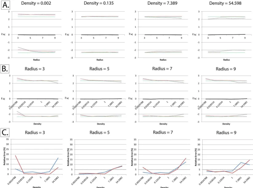
Consistent with Lagacheet al. [34], the relative error is, for the most part, below the 5% benchmark. At very small radii (radius = 3) and very high densities (>7 particles per pixel), the

relative error is higher than 5%, but still below 20%. At very high event densities, it can be seen that the empirical quantiles are closer to the mean than the Cornish-Fisher expansion, indicat-ing that under these conditions the Cornish-Fisher expansion is a good“positive”(confirming clustering/dispersion), but a poorer“negative”(ruling out clustering/dispersion).

Having shown that the extended form of Ripley’s K-function remains centralized at both small radii and high densities, we also showed that the modified form (which ignores zero pix-els) is shape-invariant.Fig 6shows thatK~retains is centralization at zero even when a large proportion of the image has been decimated.

2.

K

~

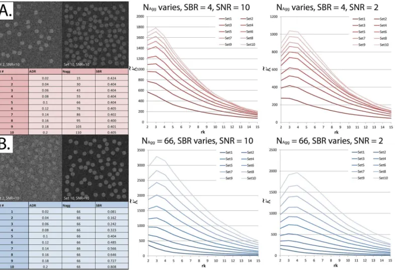
successfully ranks simulated images in the order of increasing ADR

It can be seen inFig 7thatK~increases when the proportion of particles assigned to aggregates (ADR) is increased, whether by increasing the number of aggregates or by increasing the num-ber of particles assigned to each aggregate.

Our recommendation is to not consider_K~_{to be a“hard”mathematical metric to quantify}

ADR itself. Instead, we prefer viewing_K~_{as an abstract metric that increases as either}

compo-nent of clumping increases: spatial proximity of higher intensity pixels and intensity of aggre-gates relative to the background. Thus,_K~_{is best used to rank images in the order of increasing}

aggregation under well-controlled conditions.

3. At very high densities,

½

K

~

Š

fails to correspond to the r

Even though we were able to replicate the pattern reported by Kiskowskiet alat low particle densities [39], the pattern broke down when the densities were increased to very large values. While it did remain true that as raggincreased the radius at whichK~was maximized (that is,

½K~maxŠ) also increased,½K~maxŠno longer ranged between raggand 2raggat high particle densities

(Fig 8).

at which_K~_{is maximized)? The answer is: yes, and in fact the existing methodologies for}

char-acterizing grayscale images are more abundant and intuitive than those of binary spatial distri-bution maps. Characterizing aggregates is arguably an easier process in grayscale images, since

“concrete”statistical methods can be used, including segmentation and granulometry. For example, when traditional segmentation methods are applied to the image inFig 8A, each

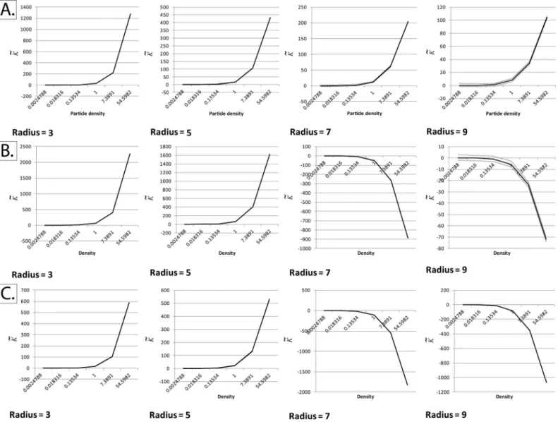
Fig 3. Unsuccessful implementations of Besag’s edge correction term at non-binary fields of view (K~with respect to event density at different radii).The normalized and centered K-function (K~), as described by Lagacheet al, was calculated at different particle intensities and radii using simulated squarefields of view measuring 256 x 256 pixels, with a homogeneous Poisson distribution of particles (Complete Spatial Randomness). Densities are expressed in particles per pixel. The black line represents the mean_K~_{and the dotted lines represent the upper and lower critical quantiles (Q01 and Q99).}

Each mean/quantile was determined using a set of 1000 simulations.Panel A: Applying Besag’s correction term only to edge pixels, by dividing the pixels within a given radius by the area of an ideal circle of the same radius. It can be seen thatK~is no longer centered around zero at high particle intensities.Panel B: Same as panel A, but dividing by a pixelated circle rather than an ideal one. Like panel A, it can be seen thatK~is no longer centered around zero at high intensities.Panel C: For comparison,K~was calculated without applying any edge correction terms. It can be seen that edge effects play a significant role at high particle intensities, makingK~deviate remarkably from zero.

particle is considered to be a separate“cluster”. On the other hand, at high particle densities (Fig 8B), a cluster would be successfully segmented.

The comparative performance of segmentation and granulometry is illustrated inFig 9. Generally-speaking, global thresholding has a more superior performance, but it performs poorer than granulometry at low SBR’s. Thus, even though½K~maxŠcannot be used to Fig 4. Unsuccessful implementations of Besag’s edge correction term at non-binary fields of view (K~with respect to radius at different event densities).The normalized and centered K-function (K~), as described by Lagacheet al, was calculated at different particle intensities and radii using simulated squarefields of view measuring 256 x 256 pixels, with a homogeneous Poisson distribution of particles (Complete Spatial Randomness). Densities are expressed in particles per pixel. The black line represents the meanK~and the dotted lines represent the upper and lower critical quantiles (Q01 and Q99). Each mean/quantile was determined using a set of 1000 simulations.Panel A: Applying Besag’s correction term only to edge pixels, by dividing the pixels within a given radius by the area of an ideal circle of the same radius. It can be seen that_K~_{is no longer centered around zero at high particle intensities.}

Panel B: Same as panel A, but dividing by a pixelated circle rather than an ideal one. Like panel A, it can be seen thatK~is no longer centered on zero at high intensities.Panel C: For comparison,_K~_{was calculated without applying any edge correction terms. It can be seen that edge effects play a signi}

ficant role at high particle intensities, makingK~deviate remarkably from zero.

approximate the size of clusters in grayscale images in the same manner that it could in binary spatial distributions, segmentation and granulometry are obvious alternatives. These methods offer the added benefit of spatial mapping of clusters as well as the ability to isolate clusters of variable sizes and shapes. The accuracy and specificity of such characterization process depends on the method used, as well as the image SBR and SNR values.

Fig 5. Successful adaptation of Besag’s boundary correction at non-binary fields of view.The normalized and centered K-function (_K~_{), as described}

by Lagacheet al, was calculated at different particle intensities and radii using simulated squarefields of view measuring 256 x 256 pixels, with a

homogeneous Poisson distribution of particles (Complete Spatial Randomness). Densities are expressed in particles per pixel. Besag’s boundary correction was applied to all particles within thefield of view and not just border pixels, as described in the text and inFig 2.Panels A and B: The black line represents the meanK~and the dotted lines represent the upper and lower critical quantiles (Q01 and Q99). In order to ensure convergence, each mean/quantile was determined using a set of 25,000 simulations. The red dotted lines represent the Cornish-Fisher expansion used to estimate the critical quantiles, as validated by Lagacheet al., while the green dotted lines represent the normal quantiles. Unlike the other unsuccessful implementations shown in Figs3and 4, meanK~remains centered on zero even at very high particle densities.Panel C: Quantifying relative error in the Cornish-Fisher expansion estimation of the empirically-determined critical quantiles.

4.

K

~

successfully ranks protein constructs in the order of increasing

soluble (diffuse) fractions

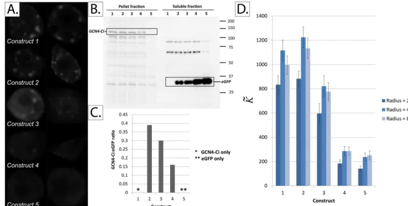
It can be seen inFig 10that the value of_K~_{successfully ranks four of thefive constructs in the}

correct order of their GCN4-Ci:eGFP co-transfection ratios. Of course, this method has its lim-itations, and it can be seen that the subtle differences between the two most-aggregated con-structs were not detected byK~.

The results are consistent with our simulation results, particularly those inFig 7A, as the main difference between various constructs is the increasing number (rather than intensity) of aggregates.

5.

K

~

successfully ranks chromatin condensation in

wt

and

crwn1 crwn2

Arabidopsis

nuclei

Our results, obtained using the same dataset as Pouletet al, confirm the findings of both Wang et aland Pouletet al;K~values of thewtconstruct were significantly higher than those of the crwn1 crwn2mutant (Fig 11). This can be attributed to the higher number of chromocentres in thewtconstruct (i.e. higher chromatin condensation state). One major advantage of using our approach is its applicability to large-scale batch processing of datasets. Manual methods, by

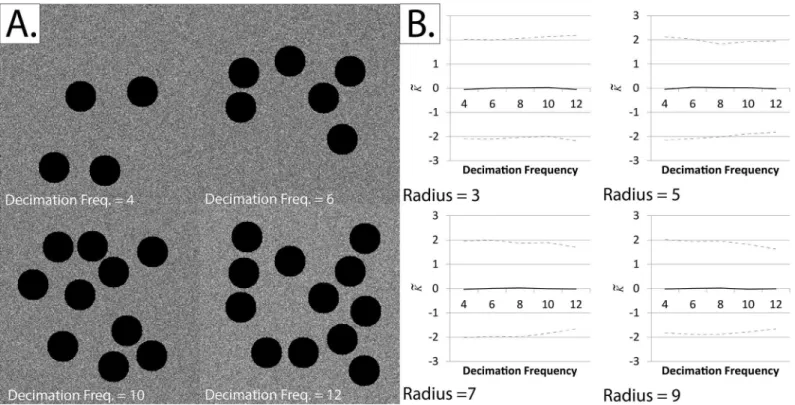
Fig 6. Testing the shape-dependence of our adaptation of Ripley’s K-function using repeated random decimation of simulated fields of view.Note that the black circular regions (black pixels) are considered to be outside the study region, and are generated to create artificial“edges”.Panel A: Sample simulated fields of view at decimation frequencies of 4, 6, 10 and 12.Panel B: The normalized and centered K-function (_K~_{) at various decimation frequencies.}

The black line represents the meanK~and the dotted lines represent the upper and lower critical quantiles (Q01 and Q99). Each mean/quantile was determined using a set of 1000 simulations. It can be seen that_K~_{remains centered on zero regardless of the decimation frequency or radius at whichK}~_was

calculated.

comparison, are rather qualitative, often unreliable, and take a lot of time therefore limiting their utility in large-scale and real-time settings. Even semi-automated methods are time-con-suming. Pouletet alreported that the time-limiting step in their analysis was the manual thresholding operation. Our method, which avoids segmentation altogether and uses an abstract index, avoids this step while still reliably reproducing the same results.

Note that since_K~_{is a spatially-variant metric that calculates the intensity distribution over}

an entirefield of view, care should be taken when any type of intensity-altering process is applied, as this will almost certainly affect the resultant_K~_{values (Fig 12). Another precaution}

to take is that images being compared should have the same bit-depth.

Moreover, it should be noted that, since_K~_{is an abstract metric that quantifies clustering}

over an entirefield of view, correct segmentation of thefield of view against a background of

Fig 7. The normalized and centered K-function (K~) increases as the Aggregate-to-Diffuse ratio (ADR) increases.EachK~result displayed represents the average of 30 simulatedfields of view using the exact same experimental parameters. Thex-axis in the right panels shows the radius at whichK~was calculated (rk).Panel A:Left—ADR was varied (the proportion of particles allocated to aggregates) by varying the number of aggregates (Nagg) while keeping

the Signal-to-Background ratio (SBR) constant. Note that the signal isadded tothe background. Since the aggregates have a pre-defined radius, SBR was not the exact same, but varied subtly due to“quantization”effects as the number of aggregates is increased.Right—As ADR increases,K~increases. This remains true at SNR = 2.Panel B:Left—ADR was varied by varying the SBR while keeping Naggconstant.Right—As ADR increases,K~increases. This

remains true at SNR = 2.

zeros is quintessential to its success. For example, under-segmentation of thefield of view may result in the whole cell being considered to be a“single big clump”, falsely increasing theK~ value. By contrast, over-segmentation can result in falsely low_K~_values.

While the focus of this paper has been on protein and chromatin aggregation, it should be noted that the methods described could be used to quantify aggregation in any type of 2-D grayscale image without regard to the“material”being aggregated.

Not only does an abstract aggregation metric have implications in research, it could poten-tially be useful in diagnostic pathology as well. Indeed, computer-assisted diagnostics have gained a lot of attention over the past few years, and there are numerous efforts to integrate automated image processing and analysis methods into daily anatomic pathology practice. As a matter of fact, an image processing approach is probably the only realistic method to quantify

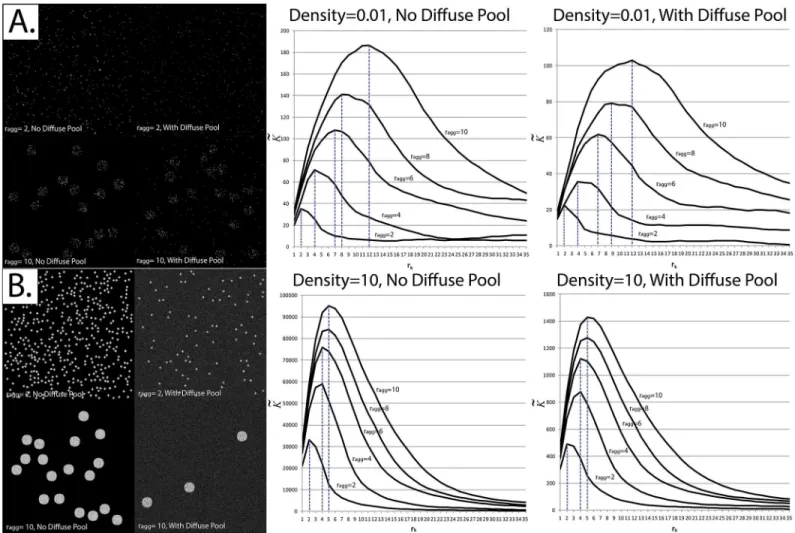
Fig 8. Correspondence between the radius at whichK~is maximized and the radius of aggregates at binary and non-binaryfields of view.EachK~ result displayed represents the average of 30 simulatedfields of view using the exact same experimental parameters.Panel A: Simulations were applied at very low event densities (0.01 particles per pixel) with and without a diffuse pool.Left—Sample simulatedfields of view. The image intensities have been rescaled for display purposes.Right—CorrespondingK~profile.Panel B: Simulations were applied at high event densities (10 particles per pixel) with and without a diffuse pool. For simulations where a diffuse pool is present, the Aggregate-to-Diffuse ratio (ADR) and Signal-to-Background ratio (SBR) were set at 0.05 and 3, respectively.Left—Sample simulatedfields of view.Right—CorrespondingK~profile.

aggregation in diagnostic pathology practice, which typically involves visual scanning of stained histopathological slides under brightfield microscopy.

Conclusions

In conclusion, we extended the use of Ripley’s K-function to grayscale (non-binary) fields of view. A simple correction to Besag’s edge correction was presented, and was successful at restoring the function’s centralization at high densities. We showed that the extended form of the function is shape-invariant, and that previously-reported correspondence between the radius at which the K-function is maximized and true cluster radius break down at high densi-ties. Simulations as well as co-transfection experiments were used to validate the function’s use as an abstract index of protein aggregation. In addition, proof-of-concept analysis was per-formed on a published chromatin condensation dataset to illustrate the generalizability of the extended form of the K-function.

Fig 9. Alternative methodologies for characterizing aggregates at non-binary fields of view.Panel A: Sample simulated field of view, corresponding ground truth and parameters used in the 10 sets generated.Panel B:Upper—First-derivative of the granulometric profile of the sample field of view shown in Panel A. It can be seen that there are four major troughs at radii 2, 5, 7 and 9 approximately corresponding to the ground truth radii of the aggregates.Lower

—Extracting aggregates with a radius of 8 pixels, by subtracting the opened image at a radius of 9 from that opened at a radius of 8. Further thresholding and processing may be performed (described in Panel C).Panel C: Demonstrating the effect of SBR on the accuracy and specificity of segmentation of

aggregates. The blue crosses represent the TET and TEE values of individual simulated fields of view (see text for a description of how TET and TEE are calculated), while the means of Sets 1 through 10 are represented by different shades of red, from darker to lighter respectively.Upper—As SBR increases, TET increases. Notice the low TET values obtained for the Sets 1–3, especially at low SNR.Lower—The result of applying the same segmentation pipeline not to the original image but to aggregates of a single radius (8 pixels) obtained using granulometric analysis (as in Panel B). The TEE values are generally lower than those of the pipeline in the upper panel. However, this method offers better results at low SBR’s (Sets 1–3).

Fig 10. Quantifying protein aggregation inDrosophilaClone 8 cells co-transfected with GCN4-Ci (a predominantly-aggregated protein) and eGFP (a predominantly-soluble protein) in various ratios.Panel A: Sample images from the five constructs tested.Panel B: Western blot showing the results of subcellular fractionation of the five constructs.Panel C: Quantification of the western blot in panel B using ImageJ.Panel D:_K~_{values for thefive constructs}

tested. The number of cells analyzed in constructs 1, 2, 3, 4 and 5 is 17, 15, 16, 27 and 20 cells, respectively. Error bars represent the standard error of the mean (SEM).

doi:10.1371/journal.pone.0144404.g010

Fig 11. Quantifying chromatin condensation inArabidopsisplant cells using the same dataset published by Pouletet al[52].Panel A: Sample images from the two constructs tested:wt(wild type) andcrwn1 crwn2mutant.Crwn1 crwn2mutant is known to have less chromocentres thanwt. Panel B:

~

Kvalues for the two constructs tested. The number of nuclei analyzed in thewtandcrwn1 crwn2constructs is 38 and 39 nuclei, respectively. Error bars represent the standard error of the mean (SEM).

Supporting Information

S1 File. Dataset used for the protein aggregation validation experiment. (RAR)

S2 File. MATLAB functions and scripts used in this paper. (RAR)

Acknowledgments

The authors would like to acknowledge with gratitude the institutional support provided by the Okinawa Institute of Science and Technology (OIST) Graduate University, as well as the

Fig 12. Distorting effect of intensity rescaling onK~values.Panel A:Left—Sample images from each of thefive constructs described inFig 10.Right— Same images after intensity normalization to occupy the full 8-bit dynamic range.Panel B:K~values for the images in Panel A at three different radii (2, 4, and 6 pixels). Note the distorting effect of intensity normalization not only on theK~values, but also on the relative ranking of images.

help provided by: Dr Mostafa Amgad (running the simulations); Dr Mohamed Abdelhak and Dr Shareef Nazzal (technical advice on programming); Dr Maha A. Temraz, Dr Ahmed E. Elmanzalawi and Dr Heba Salah (critically reviewing the manuscript and providing excellent insights and comments). The authors are grateful to the critical comments and suggestions provided by the editor and anonymous reviewers on an earlier version of this manuscript, which improved and solidified the methodology, findings and conclusions of this work.

Author Contributions

Conceived and designed the experiments: MA MMKT. Performed the experiments: MA AI MMKT. Analyzed the data: MA MMKT. Contributed reagents/materials/analysis tools: MA MMKT. Wrote the paper: MA AI MMKT.

References

1. Gatrell AC, Bailey TC, Diggle PJ, Rowlingson BS. Spatial Point Pattern Analysis and Its Application in Geographical Epidemiology. Trans Inst Br Geogr. 1996; 21: 256. doi:10.2307/622936

2. Eckel SM. Statistical analysis of spatial point patterns: Applications to economical, biomedical and eco-logical data [Internet]. Universit¨at Ulm. 2008. Available:http://www.cabnr.unr.edu/weisberg/NRES675/ Diggle2003.pdf

3. Clark PJ, Evans FC. Distance to Nearest Neighbor as a Measure of Spatial Relationships in Popula-tions. Ecology. 1954; 35: 445. doi:10.2307/1931034

4. Ripley BD. Modelling Spatial Patterns. J R Stat Soc Ser B. 1977; 39: 172–212. Available:http://www. jstor.org/stable/2984796

5. Jafari-Mamaghani M. Spatial point pattern analysis of neurons using Ripley’s K-function in 3D. Front Neuroinform. 2010; 4. doi:10.3389/fninf.2010.00009

6. Lasserre R, Charrin S, Cuche C, Danckaert A, Thoulouze M-I, de Chaumont F, et al. Ezrin tunes T-cell activation by controlling Dlg1 and microtubule positioning at the immunological synapse. EMBO J. 2010; 29: 2301–2314. doi:10.1038/emboj.2010.127PMID:20551903

7. Prior IA. Direct visualization of Ras proteins in spatially distinct cell surface microdomains. J Cell Biol. 2003; 160: 165–170. doi:10.1083/jcb.200209091PMID:12527752

8. Peterson CJ, Squiers ER. An Unexpected Change in Spatial Pattern Across 10 Years in an Aspen-White Pine Forest. J Ecol. 1995; 83: 847. doi:10.2307/2261421

9. Streib K, Davis JW. Using Ripley’s K-function to improve graph-based clustering techniques. CVPR 2011. IEEE; 2011. pp. 2305–2312. doi:10.1109/CVPR.2011.5995509

10. Kosarevych R, Rusyn B. Application of the ripley’s k-function for image segmentation. Modern Prob-lems of Radio Engineering Telecommunications and Computer Science (TCSET), 2012 International Conference. 2012. pp. 412–412. Available:http://ieeexplore.ieee.org/stamp/stamp.jsp?tp=

&arnumber=6192665&isnumber=6192411

11. Ami D, Natalello A, Lotti M, Doglia SM. Why and how protein aggregation has to be studied in vivo. Microb Cell Fact. 2013; 12: 17. doi:10.1186/1475-2859-12-17PMID:23410248

12. Minton AP. How can biochemical reactions within cells differ from those in test tubes? J Cell Sci. 2006; 119: 2863–9. doi:10.1242/jcs.03063PMID:16825427

13. Ignatova Z. Monitoring protein stability in vivo. Microb Cell Fact. 2005; 4: 23. doi: 10.1186/1475-2859-4-23PMID:16120213

14. Ross CA, Poirier MA. Protein aggregation and neurodegenerative disease. Nat Med. 2004; 10 Suppl: S10–7. doi:10.1038/nm1066PMID:15272267

15. David DC, Ollikainen N, Trinidad JC, Cary MP, Burlingame AL, Kenyon C. Widespread protein aggre-gation as an inherent part of aging in C. elegans. PLoS Biol. 2010; 8: e1000450. doi:10.1371/journal. pbio.1000450PMID:20711477

16. David DC. Aging and the aggregating proteome. Front Genet. 2012; 3: 247. doi:10.3389/fgene.2012. 00247PMID:23181070

18. García-Fruitós E, Sabate R, de Groot NS, Villaverde A, Ventura S. Biological role of bacterial inclusion bodies: a model for amyloid aggregation. FEBS J. 2011; 278: 2419–27. doi:10.1111/j.1742-4658.2011. 08165.xPMID:21569209

19. Kim W, Hecht MH. Mutations enhance the aggregation propensity of the Alzheimer’s A beta peptide. J Mol Biol. 2008; 377: 565–74. doi:10.1016/j.jmb.2007.12.079PMID:18258258

20. Ignatova Z, Gierasch LM. Monitoring protein stability and aggregation in vivo by real-time fluorescent labeling. Proc Natl Acad Sci U S A. 2004; 101: 523–8. doi:10.1073/pnas.0304533101PMID: 14701904

21. Schwarz-Romond T, Merrifield C, Nichols BJ, Bienz M. The Wnt signalling effector Dishevelled forms dynamic protein assemblies rather than stable associations with cytoplasmic vesicles. J Cell Sci. 2005; 118: 5269–77. doi:10.1242/jcs.02646PMID:16263762

22. Liapis E, Sandiford S, Wang Q, Gaidosh G, Motti D, Levay K, et al. Subcellular localization of regulator of G protein signaling RGS7 complex in neurons and transfected cells. J Neurochem. 2012; 122: 568– 81. doi:10.1111/j.1471-4159.2012.07811.xPMID:22640015

23. Wang G, Jiang J. Multiple Cos2/Ci interactions regulate Ci subcellular localization through microtubule dependent and independent mechanisms. Dev Biol. 2004; 268: 493–505. doi:10.1016/j.ydbio.2004. 01.008PMID:15063184

24. Hamilton N. Quantification and its applications in fluorescent microscopy imaging. Traffic. 2009; 10: 951–61. doi:10.1111/j.1600-0854.2009.00938.xPMID:19500318

25. Sankur B. Survey over image thresholding techniques and quantitative performance evaluation. J Elec-tron Imaging. 2004; 13: 146. doi:10.1117/1.1631315

26. Sato Y, Nakajima S, Shiraga N, Atsumi H, Yoshida S, Koller T, et al. Three-dimensional multi-scale line filter for segmentation and visualization of curvilinear structures in medical images. Med Image Anal. 1998; 2: 143–168. doi:10.1016/S1361-8415(98)80009-1PMID:10646760

27. Pop S, Dufour A, Olivo-Marin J-C. Image filtering using anisotropic structure tensor for cell membrane enhancement in 3D microscopy. 2011 18th IEEE International Conference on Image Processing. IEEE; 2011. pp. 2041–2044. 10.1109/ICIP.2011.6115880

28. Haralick RM. Statistical and structural approaches to texture. Proc IEEE. 1979; 67: 786–804. doi:10. 1109/PROC.1979.11328

29. Carpenter AE, Jones TR, Lamprecht MR, Clarke C, Kang IH, Friman O, et al. CellProfiler: image analy-sis software for identifying and quantifying cell phenotypes. Genome Biol. 2006; 7: R100. doi:10.1186/ gb-2006-7-10-r100PMID:17076895

30. Jones TR, Carpenter AE, Lamprecht MR, Moffat J, Silver SJ, Grenier JK, et al. Scoring diverse cellular morphologies in image-based screens with iterative feedback and machine learning. Proc Natl Acad Sci U S A. 2009; 106: 1826–31. doi:10.1073/pnas.0808843106PMID:19188593

31. Schneider CA, Rasband WS, Eliceiri KW. NIH Image to ImageJ: 25 years of image analysis. Nat Meth-ods. 2012; 9: 671–5. Available:http://www.ncbi.nlm.nih.gov/pubmed/22930834PMID:22930834 32. Besag JE. Comments on Ripley’s paper. J R Stat Soc B. 1977; 39: 193–195.

33. Ehrlich M, Boll W, van Oijen A, Hariharan R, Chandran K, Nibert ML, et al. Endocytosis by Random Initi-ation and StabilizIniti-ation of Clathrin-Coated Pits. Cell. 2004; 118: 591–605. doi:10.1016/j.cell.2004.08. 017PMID:15339664

34. Lagache T, Lang G, Sauvonnet N, Olivo-Marin J-C. Analysis of the Spatial Organization of Molecules with Robust Statistics. Rappoport JZ, editor. PLoS One. 2013; 8: e80914. doi:10.1371/journal.pone. 0080914PMID:24349021

35. Waters JC. Accuracy and precision in quantitative fluorescence microscopy. J Cell Biol. 2009; 185: 1135–1148. doi:10.1083/jcb.200903097PMID:19564400

36. Svoboda D, Kaš_{ík M, Ma}š_{ka M, Hubený J, Stejskal S, Zimmermann M. On Simulating 3D Fluorescent}

Microscope Images. Computer Analysis of Images and Patterns. Berlin, Heidelberg: Springer Berlin Heidelberg; pp. 309–316. doi:10.1007/978-3-540-74272-2_39

37. Rooms F, Philips W, Lidke DS. Simultaneous degradation estimation and restoration of confocal images and performance evaluation by colocalization analysis. J Microsc. 2005; 218: 22–36. doi:10. 1111/j.1365-2818.2005.01455.xPMID:15817060

38. Smal I, Loog M, Niessen W, Meijering E. Quantitative comparison of spot detection methods in fluores-cence microscopy. IEEE Trans Med Imaging. 2010; 29: 282–301. doi:10.1109/TMI.2009.2025127 PMID:19556194

40. Sternberg. Biomedical Image Processing. Computer (Long Beach Calif). 1983; 16: 22–34. doi:10. 1109/MC.1983.1654163

41. Kapur JN, Sahoo PK, Wong AKC. A new method for gray-level picture thresholding using the entropy of the histogram. Comput Vision, Graph Image Process. 1985; 29: 273–285. doi:10.1016/0734-189X (85)90125-2

42. Bovik AC, Aggrawal SJ, Merchant F, Kim NH, Diller KR. Automatic area and volume measurement from digital biomedical images. In: Hader DP, editor. Image Analysis: Methods and Applications, Sec-ond Edition. 2, illustr. CRC Press, 2000; 2003. pp. 38–42.

43. Dougherty ER, Kraus EJ, Pelz JB. Image Segmentation By Local Morphological Granulometries. 12th Canadian Symposium on Remote Sensing Geoscience and Remote Sensing Symposium,. IEEE; pp. 1220–1223. doi:10.1109/IGARSS.1989.576052

44. The Mathworks Inc. USA. Granulometry of snowflakes. In: MATLAB Documentation [Internet]. [cited 9 Sep 2015]. Available:http://www.mathworks.com/help/images/examples/granulometry-of-snowflakes. html

45. Dima AA, Elliott JT, Filliben JJ, Halter M, Peskin A, Bernal J, et al. Comparison of segmentation algo-rithms for fluorescence microscopy images of cells. Cytometry A. 2011; 79: 545–59. doi:10.1002/cyto. a.21079PMID:21674772

46. Zijdenbos AP, Dawant BM, Margolin RA, Palmer AC. Morphometric analysis of white matter lesions in MR images: method and validation. IEEE Trans Med Imaging. 1994; 13: 716–24. doi:10.1109/42. 363096PMID:18218550

47. Aza-Blanc P, Ramírez-Weber F-A, Laget M-P, Schwartz C, Kornberg TB. Proteolysis That Is Inhibited by Hedgehog Targets Cubitus interruptus Protein to the Nucleus and Converts It to a Repressor. Cell. 1997; 89: 1043–1053. doi:10.1016/S0092-8674(00)80292-5PMID:9215627

48. Ruel L, Rodriguez R, Gallet A, Lavenant-Staccini L, Thérond PP. Stability and association of Smooth-ened, Costal2 and Fused with Cubitus interruptus are regulated by Hedgehog. Nat Cell Biol. 2003; 5: 907–913. doi:10.1038/ncb1052PMID:14523402

49. Zhang Q, Shi Q, Chen Y, Yue T, Li S, Wang B, et al. Multiple Ser/Thr-rich degrons mediate the degrada-tion of Ci/Gli by the Cul3-HIB/SPOP E3 ubiquitin ligase. Proc Natl Acad Sci. 2009; 106: 21191–21196. doi:10.1073/pnas.0912008106PMID:19955409

50. Peel DJ, Milner MJ. The expression of PS integrins in Drosophila melanogaster imaginal disc cell lines. Roux’s Arch Dev Biol. 1992; 201: 120–123. doi:10.1007/BF00420423

51. Otsu N. A Threshold Selection Method from Gray-Level Histograms. IEEE Trans Syst Man Cybern. 1979; 9: 62–66. doi:10.1109/TSMC.1979.4310076

52. Poulet A, Arganda-Carreras I, Legland D, Probst AV, Andrey P, Tatout C. NucleusJ: an ImageJ plugin for quantifying 3D images of interphase nuclei. Bioinformatics. 2015; 31: 1144–1146. doi:10.1093/ bioinformatics/btu774PMID:25416749