Flow of a Second Grade Fluid over an Oscillating Vertical
Plate
Farhad Ali1, Ilyas Khan1,2, Sharidan Shafie1*
1Department of Mathematical Sciences, Faculty of Science, Universiti Teknologi Malaysia, Johor Bahru Johor, Malaysia,2College of Engineering Majmaah University, Majmaah, Kingdom of Saudi Arabia
Abstract
Closed form solutions for unsteady free convection flows of a second grade fluid near an isothermal vertical plate oscillating in its plane using the Laplace transform technique are established. Expressions for velocity and temperature are obtained and displayed graphically for different values of Prandtl number Pr, thermal Grashof numberGr, viscoelastic parametera, phase anglevtand timet. Numerical values of skin frictiont0and Nusselt number Nu are shown in tables. Some well-known solutions in literature are reduced as the limiting cases of the present solutions.
Citation:Ali F, Khan I, Shafie S (2014) Closed Form Solutions for Unsteady Free Convection Flow of a Second Grade Fluid over an Oscillating Vertical Plate. PLoS ONE 9(2): e85099. doi:10.1371/journal.pone.0085099
Editor:Enrique Hernandez-Lemus, National Institute of Genomic Medicine, Mexico
ReceivedJuly 29, 2013;AcceptedNovember 22, 2013;PublishedFebruary 14, 2014
Copyright:ß2014 Ali et al. This is an open-access article distributed under the terms of the Creative Commons Attribution License, which permits unrestricted use, distribution, and reproduction in any medium, provided the original author and source are credited.
Funding:These authors have no support or funding to report.
Competing Interests:The authors have declared that no competing interests exist. * E-mail: [email protected]
Introduction
It is well known that Newtonian fluids such as air, water, ethanol, benzene and mineral oils form a basis for classical fluid mechanics. However, many important fluids, such as blood, polymers, paint, and foods show non-Newtonian behavior. Due to the diversity of non-Newtonian fluids in nature no unique relationship is available in the literature that can describe the rheology of all the non-Newtonian fluids. Of course, the mathematical systems for non-Newtonian fluids are of higher order and complicated in comparison to the Newtonian fluids. Therefore, a variety of constitutive equations have been suggested to predict the behavior of non-Newtonian fluids. Despite of all these difficulties, the recent researchers in the field have made valuable contributions in study of flows of non-Newtonian fluids [1–12]. Amongst the different categorizations of non-Newtonian fluids, there is one simplest model of differential type fluids known as second grade fluid [13,14]. Keeping the importance of non-Newtonian fluids in mind, for the present problem, we have chosen second grade fluid as a non-Newtonian fluid. Amongst the different studies on second grade fluids [15–25], Nazar et al. [26] provided some interesting results. They considered the second grade fluid over an oscillating plate and obtained exact solutions using the Laplace transform technique, expressed them as the sum of steady-state and transient solutions. Recently, Farhad et al. [27] extended the work of Nazar et al. [26] by considering the second grade fluid to be electrically conducting and passes through a porous medium. As a special case, it is observed that their results in the absence of MHD and porosity effects are reduced to those obtained by Nazar et al. [26].
On the other hand free convection is a common process in nature and has numerous applications and occurrences in industry. It is a major cause of atmospheric and oceanic circulation
and plays an important role in the passive emergency cooling systems of advanced nuclear reactors. Furthermore, free convec-tion flows of non-Newtonian fluids with heat transfer play an important role in many industrial systems. For example, there are many process in which thermal energy is transferred from an object through the physical contact with heat transfer fluids at a temperature colder than the object. Industrial refrigeration or heating, chemical manufacturing, breweries, ventilation and air conditioning, ice rinks and engine cooling, environmental chambers, oil and gas industry and, food and pharmaceutical are some examples of such applications [28–30]. Besides that, the Stokes’ second problem for the flow of an incompressible fluid over an oscillating plane is of great importance in the literature of fluid dynamics. It admits an exact analytical solution [31]. The Stokes’ or Rayleigh problem is not only of fundamental theoretical interest but it also occurs in many applied problems [32,33].
Pop and Watanabe [34] investigated the effects of suction and injection on the free convection flow from vertical cone with uniform surface heat flux with fixed value of Pr = 0.7 and obtained numerical solutions. Kafoussias [35] studied free convection magnetohydrodynamic flows through porous medium and ob-tained numerical solutions for constant viscosity. In the investiga-tions [34,35], the coefficients of viscosity are assumed constant. However, it is observed the coefficients of viscosity for most fluids may depend on temperature [36]. Many investigations have been reported into the problem of free convection heat transfer along a vertical surface with temperature dependent viscosity for different heating conditions [37–41]. Jang and Lin [42] studied the role of temperature-dependent viscosity in laminar free convection flow adjacent to a vertical surface with uniform heat flux.
concerning the constant property effects on free convection flow of second grade fluid over the vertical isothermal plate. So, it is necessary to carry out the study on free convection flows of second grade fluid with exact solutions for the free convection flow of second grade. Exact solutions on the other hand are needed not only for the technical relevance of the flows but are also significant for a variety of other reasons such as they can be used as a benchmark by numerical solvers and for checking the stability of their solutions. Therefore, the main purpose of the present investigation is to study the unsteady free convection flow of a second grade fluid past an isothermal vertical plate oscillating in its plane with constant viscosity [34,35], and to obtain the exact solutions using the Laplace transform technique. The present problem is the extension of Nazar et al. [26]. However, it is rather complicated due to the presence of free convection term in the momentum equation which makes the momentum and energy equations coupled with each others. Hence the present solutions are more general compared to the solutions existing in the literature.
Formulation of the Problem
Following Fosdick and Rajagopal [13], the Cauchy stress tensor
T in a homogeneous incompressible fluid of second grade is related to the fluid motion in the following form
T~{pIzmA1za1A2za2A21, ð1Þ
where pis the scalar pressure, I is the identity tensor,m is the coefficient of viscosity, a1 and a2 are the material moduli
commonly referred to as the normal stress moduli andA1 andA2
stand for the first two tensor of Rivlin and Ericksen defined by
A1~LzLT, A2~dA1
dt zA1LzL
T
A1: ð2Þ
According to Fosdick and Rajagopal [13] and Dunn and Fosdick [14] the model (1) required to be compatible with thermodynamics in the sense that all motions satisfy the Clausius-Duhem inequality and the assumption that the specific Helmholtz free energy is a minimum in equilibrium at constant temperature then, the material moduli must satisfy the following conditions
m§0, a1§0, a1za2~0: ð3Þ
Now let us consider the unsteady free convection flow of a second grade fluid near an isothermal vertical plate situated in the
x,z
ð Þ plane of a Cartesian coordinate systemx,y andz: Initially, both the plate and fluid are at rest with constant temperatureT?: At timet~0z
, the plate starts motion in its plane with oscillating velocity and then transmitted to the fluid. The temperature of the plate immediately raises toTw and thereafter maintains constant.
Owing to the shear, the fluid is gradually moved and its velocity is of the form
v~v(y;t)~u(y,t)i; ð4Þ
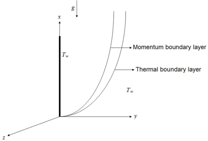
whereiis the unit vector in the flow direction as shown in Fig. 1. In the view of the above assumptions and using the usual Boussinesq approximation, the momentum and energy equations for the incompressible flow of a second grade fluid are
Figure 1. Physical geometry and coordinates system.
rLu Lt~m
L2u
Ly2za1 L3u
Ly2LtzgbTðT{TwÞ, ð5Þ
rcp
LT
Lt ~k L2T
Ly2: ð6Þ
The appropriate initial and boundary conditions
u y,0ð Þ~0, T y,0ð Þ~T?, yw0,
uð Þ0,t ~UH tð Þcosðv1tÞ or uð Þ0,t ~Usinðv1tÞ,tw0,
Tð Þ0,t ~Tw, tw0,
uð?,tÞ~0, Tð?,tÞ~T?,tw0, ð7Þ
where u~u y,tð Þ denotes the fluid velocity in the x{direction, T~T y,tð Þ is the temperature,r is the constant density of the fluid,m is the viscosity,a1 is the second grade parameter,bT is
the volumetric coefficient of thermal expansion,g is the acceleration due to gravity,cp is the specific heat capacity,k is
the thermal conductivity,T? is the free stream temperature,v1
the frequency of the velocity of the wall andH tð Þis the Heaviside unit step function.
By introducing the following dimensionless variables
v~u
U, j~ U
ny, t~ U2
n t, v~ n
U2v1, h~
T{T?
Tw{T?
, ð8Þ
the system of equationsð Þ5{ð Þ7 reduces to
Lv
Lt{ L2v
Lj2{a L3v
Lj2Lt{Grh~0, ð9Þ
PrLh
Lt~ L2h
Lj2, ð10Þ
vðj,tÞ~0; h jð ,tÞ~0; tƒ0,
vð0,tÞ~Hð Þt cosðvtÞ or
vð0,tÞ~sinðvtÞ, h jð ,tÞ~1 tw0,
vð?,tÞ~0, hð?,tÞ~0, tw0, ð11Þ
where
a~a1U 2
rn2 , Gr~
gbTnðTw{T?Þ
U3 , Pr~
mcp
k :
Hereais the dimensionless second grade parameter,Gris the thermal Grashof number andPris the Prandtl number.
Solution of the Problem
We solve the governing equations in exact form by the Laplace transform technique and their solutions in the transform ðy,qÞ -plane are given by
vvcðj,qÞ~
q
q2zv2exp {
j ffiffiffi a
p
ffiffiffiffiffiffiffiffiffiffiq
qzb r
z a
q2ðq{bÞexp {
j ffiffiffi a
p
ffiffiffiffiffiffiffiffiffiffiq
qzb r
{ a
q2ðq{bÞexp {j ffiffiffiffiffiffiffiffi
Prq
p
, ð12Þ
vvsðj,qÞ~
v
q2zv2exp {
j ffiffiffi a
p
ffiffiffiffiffiffiffiffiffiffiq
qzb r
z a
q2ðq{bÞexp {
j ffiffiffi a
p ffiffiffiffiffiffiffiffiffiffiq
qzb r
{ a
q2ðq{bÞexp {j ffiffiffiffiffiffiffiffi
Prq
p
, ð13Þ
h h jð ,qÞ~1
qexp {j
ffiffiffiffiffiffiffiffi
Prq
p
, ð14Þ
where the subscriptscandsin Eqs. (12) and (13) refer to cosine and sine oscillations of the plate and
a~ Gr aPr, b~
1 a, b~
1{Pr
aPr , Pr=1:
We split Eq. (12) in the following forms
vv1ð Þq~
q
q2zv2, vv4ðj,qÞ~
a
q2ðq{bÞexp {j ffiffiffiffiffiffiffiffi Prq p , vv2ð Þq~
a q2ðq{bÞ,
ð15Þ
vv3ðj,qÞ~exp {
j ffiffiffi a
p ffiffiffiffiffiffiffiffiffiffiq
qzb r
: ð16Þ
Let us we denote
v1ð Þt~L{1fvv1ð Þqg, v2ð Þt~L{1fvv2ð Þqg,
v3ðj,tÞ~L{1fvv3ðj,qÞg, v4ðj,tÞ~L{1fvv4ðj,qÞg,
whereL{1is denoting the inverse Laplace transform.
In order to find the inverse Laplace transform of Eq. (12), we write the velocityvcðj,tÞ as a convolution product (see theorem
(A1) from Appendix S1).
vc(j,t)~
ðt
0
v1ðt{sÞv3ðj,sÞdsz ðt
0
v2ðt{sÞv3ðj,sÞds{v4ðj,tÞ:ð17Þ
Laplace inversion of Eq.ð Þ15 leads to the following expressions.
v1ð Þt~cosðvtÞ, v2ð Þt~
a e bt{bt{1
b2 , ð18Þ
v4ðj,tÞ~ aebt 2b2
e{j ffiffiffiffiffiffi
bPr p
erfc j ffiffiffiffiffi
Pr p
2 ffiffiffi t p {pffiffiffiffiffibt
!
zej ffiffiffiffiffiffi
bPr p
erfc j ffiffiffiffiffi
Pr p
2 ffiffiffi t p zpffiffiffiffiffibt
!
" #
{a
b tz j2Pr
2
!
erfc j
ffiffiffiffiffi
Pr
p
2pffiffiffit ! {j ffiffiffiffiffiffiffiffi Prt p ffiffiffi p
p e{j2 Pr4t
" #
{ a
b2erfc
jpffiffiffiffiffiPr 2pffiffiffit
! : ð19Þ {a
b2erfc
In order to find v3ðj,tÞ,we use the inversion formula of
compound functions (A2) and some of the known results (A4)-(A7) from Appendix S1, consequently Eq. (16) results.
v3ðj,tÞ~
jd tð Þ 2 ffiffiffiffiffiffi ap
p ð?
0
exp {j2 4au{u
u ffiffiffi
u
p du
zje
{bt ffiffiffi
b p 2 ffiffiffiffiffiffiffiffi apt p ð? 0
exp{4ja2u{u u I1 2
ffiffiffiffiffiffiffiffi but p
du,
ð20Þ
wheredð Þ: is the Dirac delta function andI1ð Þ: is the modified
Bessel function of the first kind of order one. Using Eqs. (18)–(20) into Eq. (17), keeping in mind (A3) from Appendix S1, we get
ð ?
t
fðj,t,sÞds~ ð ?
0
fðj,t,sÞds{ ð ?
t
fðj,t,sÞds ð23Þ
and use formulae (A8)-(A10) from Appendix S1, we obtain
vc(j,t)~vcs(j,t)zvct(j,t), vs(j,t)~vss(j,t)zvst(j,t), ð24Þ where the steady state solutions are written as
vc(j,t)~
jHð Þt cosðvtÞ 2 ffiffiffiffiffiffi
ap
p
ð?
0
exp {j2 4au{u
u ffiffiffi
u
p duzjHð Þt
ffiffiffi b p 2 ffiffiffiffiffiffi ap p ðt 0 ð? 0
cosðvt{vsÞexp {j2
4au{u{bs
u ffiffi
s
p
I1 2 ffiffiffiffiffiffiffi bus
p
du dszaj e
bt{bt{1
2b2 ffiffiffiffiffiffi ap
p
ð?
0
exp{4ja2u{u u ffiffiffi
u
p du
zaj ffiffiffi b
p
ebt
2b2 ffiffiffiffiffiffi ap p ðt 0 ð? 0
exp {j2
4au{u{bs{bs
{b(t{s){1
h i
u ffiffi
s
p I1 2
ffiffiffiffiffiffiffi bus p du ds {ae bt
2b2 e
{jpffiffiffiffiffiffibPr
erfc j
ffiffiffiffiffi
Pr
p
2 ffiffiffi t
p {pffiffiffiffiffibt ! "
zej ffiffiffiffiffiffibPr p
erfc j
ffiffiffiffiffi
Pr
p
2 ffiffiffi t
p zpffiffiffiffiffibt !#
za
b tz j2Pr
2
!
erfc j
ffiffiffiffiffi
Pr
p
2pffiffiffit ! {j ffiffiffiffiffiffiffiffi Prt p ffiffiffi p
p e{j2 Pr
4t
" #
za
b2erfc
j ffiffiffiffiffi
Pr
p
2pffiffiffit !
:
Similarly for the sine oscillations of the plate the corresponding expression of velocity is given by
vs(j,t)~
jsinðvtÞ 2 ffiffiffiffiffiffi
ap
p
ð?
0
exp {j2 4au{u
u ffiffiffi
u
p duz j
ffiffiffi b p 2 ffiffiffiffiffiffi ap p ðt 0 ð? 0
sinðvt{vsÞexp {j2 4au{u{bs
u ffiffi
s
p I1 2
ffiffiffiffiffiffiffi bus
p
du ds
zaj e
bt{bt{1
2b2pffiffiffiffiffiffiap ð?
0
exp{4ja2u{u upffiffiffiu duz
aj ffiffiffi b
p
ebt
2b2pffiffiffiffiffiffiap ðt
0 ð?
0
exp{4ja2u{u{bs{bs{b(t{s){1
h i
upffiffis
I1 2 ffiffiffiffiffiffiffi bus
p
du ds{ae
bt
2b2 e
{jpffiffiffiffiffiffibPr
erfc j
ffiffiffiffiffi
Pr
p
2 ffiffiffi t
p {pffiffiffiffiffibt !
z "
ejpffiffiffiffiffiffibPr
erfc j
ffiffiffiffiffi
Pr
p
2 ffiffiffi t
p zpffiffiffiffiffibt !#
za
b tz j2Pr
2
!
erfc j
ffiffiffiffiffi
Pr
p
2pffiffiffit ! {j ffiffiffiffiffiffiffiffi Prt p ffiffiffi p
p e{j2 Pr4t
" #
za
b2erfc
jpffiffiffiffiffiPr 2pffiffiffit
! :
(22)
The starting solutions ofvc(j,t) andvs(j,t)given by Eqs. (21)
and (22) are rather complicated. Therefore, we derive approxi-mate expressions for these velocities corresponding to small and large values of time. This time is important, especially for those who need to eliminate transients from their rheological measure-ments [26]. In order to determine this time, we need first to write the starting solutions as the sum of the steady state and transient solutions. Therefore, we decompose the integrals from Eqs. (21) and (22) under the form
vcs(j,t)~Hð Þt e{mjcosðvt{njÞ, ð25Þ
vss(j,t)~e{mjsinðvt{njÞ, ð26Þ
which are periodic in time and independent of the initial condition. The transient solutions in equivalent but more suitable forms are written as
in which
m2~ v
2 1h zðavÞ2i
ffiffiffiffiffiffiffiffiffiffiffiffiffiffiffiffiffiffiffi
1zðavÞ2 q
zav
and
n2~ v
2 1h zðavÞ2i
ffiffiffiffiffiffiffiffiffiffiffiffiffiffiffiffiffiffiffi
1zðavÞ2 q
{av
:
The inverse Laplace transform of Eq. (14) gives the required temperature as
h jð ,tÞ~erfc j
ffiffiffiffiffi Pr p 2 ffiffiffi t p !
: ð29Þ
It is important to note that the steady state solutions (25) and (26) are independent of thermal effects whereas, the transient
solutions (27) and (28) contain the thermal effects due to the presence of free convection term. Therefore, these transient solutions can be written as a sum of the mechanicalvctmeðj,tÞ and
thermalvctthðj,tÞ components as below
vctðj,tÞ~vctmeðj,tÞzvctthðj,tÞ, ð30Þ
vstðj,tÞ~vstmeðj,tÞzvstthðj,tÞ, ð31Þ
where
vctmeðj,tÞ~{
Hð Þtj ffiffiffi b p 2 ffiffiffiffiffiffi ap p ð? j 2pffiffit
ð?
0
cosðvt{vsÞexp { j 2
4au{u{bs
!
upffiffis I1 2 ffiffiffiffiffiffiffi bus
p
du ds
ð32Þ
vstmeðj,tÞ~{
Hð Þtj ffiffiffi b
p
2pffiffiffiffiffiffiap
ð?
j 2pffiffit
ð?
0
sinðvt{vsÞexp { j 2
4au{u{bs
!
u ffiffi
s
p I1 2
ffiffiffiffiffiffiffi bus
p
du ds
ð33Þ
vctðj,tÞ~{
Hð Þtj ffiffiffi b p 2 ffiffiffiffiffiffi ap p ð? j 2pffiffit
ð?
0
cosðvt{vsÞexp{4ja2u{u{bs u ffiffi
s
p I1 2
ffiffiffiffiffiffiffi bus
p
du dsz
aexp {pjffiffia
ebt{bt{1
b2
z a
b2erfc
jpffiffiffiffiffiPr 2pffiffiffit
! { 2a ffiffiffiffiffiffi ap p e bt
b2{
t b{ 1 b2 ð? j 2pffiffit
exp {s 2
a{ j2 4s2
!
dsz 2a ffiffiffiffiffiffi ap
p e
bt
b2{
t b{ 1 b2 ð? j 2pffiffit
exp {s 2
a{ b bzb
j2 4s2
!
ds
z aj ffiffiffi b
p
2bpffiffiffiffiffiffiap ð?
j 2pffiffit
ð?
0 ffiffi
s
p
cosðvt{vsÞexp {j2
4au{u{bs
u I1 2
ffiffiffiffiffiffiffi bus
p
du ds{ae
bt
2b2 e
{jpffiffiffiffiffiffibPr
erfc j
ffiffiffiffiffi
Pr
p
2pffiffiffit { ffiffiffiffiffi
bt
p !
"
zejpffiffiffiffiffiffibPrerfc j
ffiffiffiffiffi
Pr
p
2pffiffiffitz ffiffiffiffiffi
bt
p !#
za
b tz j2Pr
2
!
erfc j
ffiffiffiffiffi
Pr
p
2pffiffiffit ! {j ffiffiffiffiffiffiffiffi Prt p ffiffiffi p
p e{j2 Pr
4t
" #
, (27)
vstðj,tÞ~{
j ffiffiffi b p 2 ffiffiffiffiffiffi ap p ð? j 2pffiffit
ð?
0
sinðvt{vsÞexp {j2 4au{u{bs
u ffiffi
s
p I1 2
ffiffiffiffiffiffiffi bus
p
du ds{ 2a ffiffiffiffiffiffi ap
p e
bt
b2{
t b{ 1 b2 ð? j 2pffiffit
exp {s 2 a{ j2 4s2 ! ds z 2a ffiffiffiffiffiffi ap p e bt
b2{
t b{ 1 b2 ð? j 2pffiffit
exp {s 2
a{ b bzb
j2
4s2 !
dsz aj ffiffiffi b p 2b ffiffiffiffiffiffi ap p ð? j 2pffiffit
ð?
0 ffiffi
s
p
sinðvt{vsÞexp{4ja2u{u{bs u ffiffi
s
p
I1 2 ffiffiffiffiffiffiffi bus
p
du ds{ae
bt
2b2 e
{jpffiffiffiffiffiffibPr
erfc j
ffiffiffiffiffi
Pr
p
2 ffiffiffi t
p {pffiffiffiffiffibt !
z "
ejpffiffiffiffiffiffidPrerfc j
ffiffiffiffiffi
Pr
p
2 ffiffiffi t
p zpffiffiffiffiffidt !#
za
b tz j2Pr
2
!
erfc j
ffiffiffiffiffi
Pr
p
2pffiffiffit ! {j ffiffiffiffiffiffiffiffi Prt p ffiffiffi p
p e{j2 Pr
4t
" #
z
aexp {pjffiffia
ebt{bt{1
b2 z
a b2erfc
jpffiffiffiffiffiPr 2pffiffiffit
!
in which the subscriptsmeandthare used for the mechanical and
thermal parts of transient velocity.
Further, it is worth mentioning to note that solutions (21) and (22) are valid only for Pr=1, however to make these solutions valid for Pr~1, we once again derive our solutions by putting Pr~1into Eq. (14) and using it in the transform solution of Eq. (9), the starting solutions are
corresponding to the cosine and sine oscillations of the plate and
a1~
Gr
a. Now by employing the previous methodology, the starting solutions (36) and (37) can also be written as a sum of the steady-state and transient solutions.
vctthðj,tÞ~
aexp {pjffiffia
ebt{bt{1
b2 z
a b2erfc
jpffiffiffiffiffiPr 2 ffiffiffi
t
p !
{ 2affiffiffiffiffiffi ap
p e
bt
b2{
t b{ 1 b2 ð? j 2pffiffit
exp {s 2 a{ j2 4s2 ! ds z 2a ffiffiffiffiffiffi ap p e bt
b2{
t b{ 1 b2 ð? j 2pffiffit
exp {s 2
a{ b bzb
j2 4s2
!
ds
z aj ffiffiffi b
p
2bpffiffiffiffiffiffiap ð?
j 2pffiffit
ð?
0 ffiffi
s
p
cosðvt{vsÞexp {4j2
au{u{bs
u I1 2
ffiffiffiffiffiffiffi bus p du ds {ae bt
2b2 e
{jpffiffiffiffiffiffibPr
erfc j
ffiffiffiffiffi
Pr
p
2pffiffiffit { ffiffiffiffiffi
bt
p !
z "
ejpffiffiffiffiffiffibPrerfc j
ffiffiffiffiffi
Pr
p
2pffiffiffit z ffiffiffiffiffi
bt
p !#
za
b tz j2Pr
2
!
erfc j
ffiffiffiffiffi Pr p 2 ffiffiffi t p ! {j ffiffiffiffiffiffiffiffi Prt p ffiffiffi p
p e{j2 Pr4t
" #
,
(34)
vstthðj,tÞ~
aexp { jffiffi a p
ebt{bt{1
b2 z
a b2erfc
j ffiffiffiffiffi
Pr
p
2pffiffiffit ! { 2a ffiffiffiffiffiffi ap p e bt
b2{
t b{ 1 b2 ð? j 2pffiffit
exp {s 2 a{ j2 4s2 ! ds z 2a ffiffiffiffiffiffi ap p e bt
b2{
t b{ 1 b2 ð? j 2pffiffit
exp {s 2
a{ b bzb
j2 4s2
!
ds
z aj ffiffiffi b p 2b ffiffiffiffiffiffi ap p ð? 0 ð? j 2pffiffit
ffiffi
s
p
sinðvt{vsÞexp {j2
4au{u{bs
u I1 2
ffiffiffiffiffiffiffi bus p du ds {ae bt
2b2 e
{jpffiffiffiffiffiffibPr
erfc j
ffiffiffiffiffi
Pr
p
2 ffiffiffi t
p {pffiffiffiffiffibt !
z "
ej ffiffiffiffiffiffibPr p
erfc j
ffiffiffiffiffi
Pr
p
2 ffiffiffi t
p zpffiffiffiffiffibt !#
za
b tz j2Pr
2
!
erfc j
ffiffiffiffiffi Pr p 2 ffiffiffi t p ! {j ffiffiffiffiffiffiffiffi Prt p ffiffiffi p
p e{j2 Pr4t
" #
,
(35)
vcðj,tÞ~Hð Þt expð{mjÞcosðvt{njÞ{
a1
2 j4 12zj
2tzt2 !
erfc j 2 ffiffiffi
t
p
{Hð Þtj ffiffiffi b p 2 ffiffiffiffiffiffi ap p ðt 0 ð? 0
cosðvt{vsÞexp {j2
4au{u{bs
upffiffis I1 2 ffiffiffiffiffiffiffi bus
p
du ds
za1j ffiffiffi b p 4 ffiffiffiffiffiffi ap p ðt 0 ð? 0
t{s
ð Þ2exp {j2
4au{u{bs
u ffiffi
s
p I1 2
ffiffiffiffiffiffiffi bus
p
du ds
{a1j
12 ffiffiffi t p r j2 2z5t
!
e{j2
4tza1t 2e{pjffiffia
2 ,
(36)
vsðj,tÞ~expð{mjÞsinðvt{njÞ{
a1
2 j4 12zj
2tzt2 !
erfc j 2pffiffiffit
{ j ffiffiffi b p 2 ffiffiffiffiffiffi ap p ðt 0 ð? 0
sinðvt{vsÞexp{4ja2u{u{bs u ffiffi
s
p I1 2
ffiffiffiffiffiffiffi bus
p
du ds
za1j ffiffiffi b
p
4pffiffiffiffiffiffiap ðt
0 ð?
0
t{s
ð Þ2exp {j2
4au{u{bs
upffiffis I1 2 ffiffiffiffiffiffiffi bus
p
du ds
{a1j
12 ffiffiffi t p r j2 2z5t
!
e{j
2 4tza1t
Limiting Cases
Equations (21) and (22) investigate the exact solutions for the starting motion of a second grade fluid for the cosine and sine oscillations of an isothermal vertical plate respectively and Eq. (28) represents the corresponding solution for temperature of the fluid. Since the present solutions are more general and the existing published results from the literature appear as special cases by taking suitable parameters such as Grashof numberGr,frequency of oscillationsvand the second grade parameteraequal to zero.
Case-I: Solutions in the Absence of Thermal Effects In the absence of free convection, the solution of temperature (29), is unaffected by the thermal effects due to the reason that the free convection termGr is not involved there, however by taking Gr~0implies thata~0,Eqs.ð Þ21 andð Þ22 yield Eqs.ð Þ38 and
39
ð Þ as follows
vcðj,tÞ~Hð Þt expð{mjÞcosðvt{njÞ
{Hð Þtj ffiffiffi b p 2 ffiffiffiffiffiffi ap p ðt 0 ð? 0
cosðvt{vsÞ
| 1
u ffiffi
s
p exp { j
2
4au{u{bs
!
I1 2 ffiffiffiffiffiffiffi bus
p
du ds: ð38Þ
vsðj,tÞ~expð{mjÞsinðvt{njÞ{
j ffiffiffi b
p
2pffiffiffiffiffiffiap ðt
0 ð?
0
sinðvt{vsÞ
| 1
u ffiffi
s
p exp { j
2
4au{u{bs
!
I1 2 ffiffiffiffiffiffiffi bus
p
du ds, ð39Þ
which are identical to the starting solutions obtained by Nazar et al. (Eqs. (13) and (14) in [26]) describe the motion of the fluid for
small and large times. Furthermore, for a?0,m~n~ ffiffiffiffi v 2
r , the
steady parts of Eqs.ð Þ38 andð Þ39 give the well known results
ucs(y,t)~H tð Þe
{ ffiffiffiv
2 p
y
cos vt{ ffiffiffiffi v 2 r y
, ð40Þ
uss(y,t)~e
{ ffiffiffiv
2 p
y
sin vt{ ffiffiffiffi v 2 r y
, ð41Þ
which are quite identical to the published results obtained by Erdogan (Eqs.ð Þ12 andð Þ17 in [46]) and Feteca et al. (Eq.ð Þ17 in [47]).
Case-II: Solutions in the Absence of Oscillating Effects Now let us assume that the infinite plate is set into impulsive motion after time t~0z
:The thermal component of velocity vctthðj,tÞ remain unchanged while the mechanical part of velocity
vctmeðj,tÞ is effected due to the frequency of oscillationsv: So, by
takingv?0into Eq.ð Þ21 , the solution corresponding to the case
when the plate applies impulsive motion to the fluid is given by
Case-III: Solutions in the Absence of Mechanical Effects Here we assume that the infinite plate is kept at rest all the time. In this case the motion in the fluid together with heat transfer are only caused due to the presence of free convection because there is no disturbance from the bounding plate. Thus, the mechanical component of velocity is identically zero and consequently the velocity of the fluidv(j,t) reduces to the thermal component vc(j,t)~
jHð Þt 2 ffiffiffiffiffiffi ap
p ð?
0
exp{4ja2u{u u ffiffiffi
u
p duzjHð Þt ffiffiffi b p 2 ffiffiffiffiffiffi ap p ðt 0 ð? 0
exp{4ja2u{u{bs u ffiffi
s
p I1 2
ffiffiffiffiffiffiffi bus
p
du dszaj e
bt{bt{1
2b2 ffiffiffiffiffiffi ap
p
ð?
0
exp{4ja2u{u u ffiffiffi
u
p du
zaj ffiffiffi b
p
ebt
2b2 ffiffiffiffiffiffi ap p ðt 0 ð? 0
exp {j2
4au{u{bs{bs
{b(t{s){1
h i
upffiffis I1 2 ffiffiffiffiffiffiffi bus p du ds zae bt
2b2 e
{jpffiffiffiffiffiffibPr
erfc j
ffiffiffiffiffi
Pr
p
2 ffiffiffi t
p {pffiffiffiffiffibt ! "
zejpffiffiffiffiffiffibPr
erfc j
ffiffiffiffiffi
Pr
p
2 ffiffiffi t
p zpffiffiffiffiffibt !#
{a
b tz j2Pr
2
!
erfc j
ffiffiffiffiffi
Pr
p
2pffiffiffit ! {j ffiffiffiffiffiffiffiffi Prt p ffiffiffi p
p e{j2 Pr
4t
" #
z a
b2erfc
j ffiffiffiffiffi
Pr
p
2pffiffiffit !
: (42)
vs(j,t)~
ajebt{bt{1
2b2pffiffiffiffiffiffiap ð?
0
exp{4ja2u{u upffiffiffiu du
zaj ffiffiffi b
p
ebt
2b2 ffiffiffiffiffiffi ap p ðt 0 ð? 0
exp {j2
4au{u{bs{bs
{b(t{s){1
h i
u ffiffi
s
p I1 2
ffiffiffiffiffiffiffi bus p du ds zae bt
2b2 e
{jpffiffiffiffiffiffibPr
erfc j
ffiffiffiffiffi
Pr
p
2 ffiffiffi t
p {pffiffiffiffiffibt !
z "
ej ffiffiffiffiffiffibPr p
erfc j
ffiffiffiffiffi
Pr
p
2 ffiffiffi t
p zpffiffiffiffiffibt !#
{a
b tz j2Pr
2
!
erfc j
ffiffiffiffiffi
Pr
p
2pffiffiffit ! {j ffiffiffiffiffiffiffiffi Prt p ffiffiffi p
p e{j2 Pr
4t
" #
z a
b2erfc
j ffiffiffiffiffi
Pr
p
2pffiffiffit !
:
We note that the solutions obtained as limiting cases (Case-II & Case-III) are also new and not available in the literature.
Skin-Friction
The expression for dimensional skin friction in case of a second grade fluid is given as
t0~ mLu Lyza1
L2u
LyLt
" #
y~0
: ð44Þ
In dimensionless form Eq.ð Þ44 is written as
t0~ Lv
Ljza L2v
LjLt
" #
j~0
, ð45Þ
where t0~ t0
rU2:
Finally, Eq.(45)in view of Eq.(21)gives
Nusselt Number
The rate of heat transfer evaluated from Eq.ð Þ29 is given by
Nu~ ffiffiffiffiffi
Pr
p
ffiffiffiffiffi pt
p : ð47Þ
Results and Discussion
A numerical assessment for the exact solutions (21) of the present problem corresponding to the cosine oscillations of the plate and (29) is performed. Using a computational software Mathcad, the results are plotted to illustrate the interesting features of the involved parameters on the starting solution corresponding to the cosine oscillations of the plate (Figs.2{6) and temperature profiles (Fig. 6and 7) whereas Figs. 8and 9are shown for the starting and steady-state velocities corresponding to the cosine and sine oscillations of the plate. In addition Fig.10 is prepared to show the comparison of the present results with Nazar et al.
26
½ :The parameters entering into the problem are second grade parametera, Prandtl number Pr, thermal Grashof number Gr, dimensionless timet, and phase anglevt.
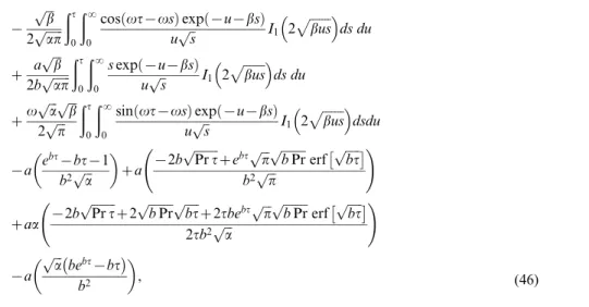
Figure 2 shows the influence ofaon the velocity fieldv(j,t). It is clear from this figure that an increase inaresults a decrease in the velocity. Physically, it is true because the higher values ofa,are having greater stability than the smaller values. This behavior ofa is quite similar to that of Sivaraj and Kumar (see Fig. 4 in [32]). Unlike [34,35], the effect of Prandtl numberPrfor four different values as Pr~0:71, 0:9, 1:5 and 7 upon velocity v(j,t) is elucidated from Fig.3. It is seen from this figure.3that in the case of heating of the plate or cooling of the fluid ðGrv0Þ, velocity v(j,t)decreases when Prandtl numberPrincreases. Physically, it is true as the Prandtl number describes the ratio between momentum diffusivity and thermal diffusivity and hence controls the relative thickness of the momentum and thermal boundary layers. AsPrincreases the viscous forces (momentum diffusivity) dominate the thermal diffusivity and consequently decreases the velocity. The influence of thermal Grashof numberGron velocity distributionv(j,t)is elucidated from Fig.4. It is clear from this figure that in the absence of thermal effect(Gr~0)when the effect
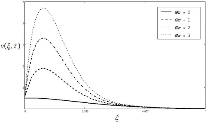
of buoyant forces is negligible and the viscous forces are dominant, the velocity tends to steady-state faster than for the values of Grw0:It can be observed that velocity increases for the increasing values ofGr:It is also true physically as the Grashof numberGr describes the ratio of bouncy forces to viscous forces. Therefore, an increase in the values ofGrleads to increase in buoyancy forces, consequently velocity increases.
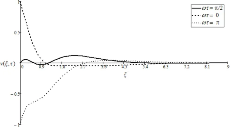
The effect of dimensionless timeton velocityv(j,t)is illustrated from Fig. 5: It can be seen from this figure that velocity is a decreasing function of t. The effect of phase angle vt upon velocityv(j,t)is elucidated from Fig.6:It is observed that velocity v(j,t) is fluctuating between21 and 1, tending to zero for large
values of independent variabley:It is clear from this figure that the obtained solution (21) satisfies the corresponding boundary conditions given in Eq. (11). Hence this provides a useful mathematical check. The influence of Prandtl number Pr on temperature profileh(j,t)is shown in Fig.7. Four different values of Pr~0:015, 0:71, 1 and 7 are chosen. They physically correspond to mercury, electrolyte, air and water respectively. It is found that temperature decreases whenPris increased. AsPris the ratio of momentum diffusivity (kinematic viscosity) to that of t0~{mcosðvtÞznsinðvtÞzanvcosðvtÞzamvsinðvtÞ
{ ffiffiffi b
p
2pffiffiffiffiffiffiap ðt
0 ð?
0
cosðvt{vsÞexpð{u{bsÞ
upffiffis I1 2 ffiffiffiffiffiffiffi bus
p
ds du
z a
ffiffiffi b
p
2b ffiffiffiffiffiffi ap
p ðt
0 ð?
0
sexpð{u{bsÞ
u ffiffi
s
p I1 2
ffiffiffiffiffiffiffi bus
p
ds du
zv ffiffiffi a
p ffiffiffi b
p
2 ffiffiffi p
p ðt
0
ð?
0
sinðvt{vsÞexpð{u{bsÞ
u ffiffi
s
p I1 2
ffiffiffiffiffiffiffi bus
p
dsdu
{a e
bt{bt{1
b2pffiffiffia
za {2b
ffiffiffiffiffiffiffiffi
Prt
p
zebt ffiffiffi p
p ffiffiffiffiffiffiffiffi
bPr
p
erf ffiffiffiffiffi
bt
p
b2pffiffiffip
!
zaa {2b ffiffiffiffiffiffiffiffi
Prt
p
z2pffiffiffiffiffiffiffiffibPrpffiffiffiffiffibtz2tbebt ffiffiffi p
p ffiffiffiffiffiffiffiffi
bPr
p
erfpffiffiffiffiffibt
2tb2 ffiffiffi a
p
!
{a
ffiffiffi a
p
bebt{bt
b2
Figure 2. Velocity profiles for different values ofawhenPr~0:71,Gr~0:5,v~2,vt~p
3,andt~1: doi:10.1371/journal.pone.0085099.g002
Figure 3. Velocity profiles for different values ofPrwhena~0:2,Gr~{0:2,v~5,vt~p
thermal diffusivity, so the increase in Pr is actually increase in viscous forces (viscosity) which results a decrease in temperature profile. The effect of dimensionless time t on the temperature
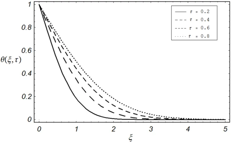
profilesh(j,t)is shown in Fig.8:It can be seen from the figure that the effect of timeton temperatureh(j,t)is quite opposite to the Prandtl numberPras observed in Fig. 7.
Figure 4. Velocity profiles for different values ofGrwhena~0:8,Pr~0:71,v~0:5,vt~p
3,andt~1: doi:10.1371/journal.pone.0085099.g004
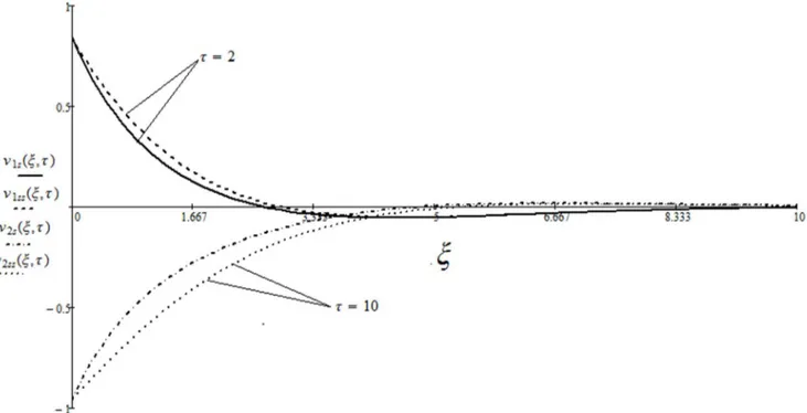
A very important problem regarding the technical applicability of the starting solutions is to find the approximate time after which the fluid is moving according to the steady-state solutions. More exactly, in practice it is necessary to know the required time to attain the steady state [26]. For this purpose, the variations of the corresponding starting and steady-state velocities with the distance from the wall are depicted in Figs. 9 and 10. At small values of time, the difference between unsteady and steady-state velocities is large enough. This difference rapidly decreases and it can be clearly seen from the figures that the required time(t~6)to reach the steady-state for the cosine oscillations of the boundary is
smaller than that for the sine oscillations(t~10). A comparative study of the present solution (21) corresponding to the cosine oscillations of the plate is provided in Fig.11with published results of Nazar et al. (Eq. (13) in [26]) It is found that in the absence of free convection (Gr~0) the present results are identical with those of Nazar et al. [26].
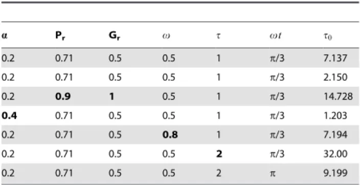
The numerical results for skin frictiont0 are shown in Table
1for various embedded parameters. It is found that the skin friction decreases whena is increased. On the other hand, the influence of Prandtl number Pr on skin friction shows that t0decreases when Pr increases whereas it increases for large Figure 6. Velocity profiles for different values ofvtwhenPr~0:71,a~0:2,Gr~0:5,v~1andt~1:
doi:10.1371/journal.pone.0085099.g006
Figure 8. Temperature profiles for different values oftwhenPr~0:71: doi:10.1371/journal.pone.0085099.g008
Figure 9. Variations of the starting and steady-state solutions with the distance from the wall, for the cosine oscillations of the boundary, corresponding to relation (21) curvesv1sðj,tÞ,v2sðj,tÞand relation (25) curvesv1ssðj,tÞ,v2ssðj,tÞ, whenGr~0,v~0:5and a~0:8:
values ofGr,tandvt:The effects ofPrandton Nusselt number Nu are studied numerically in Table 2: It is found that Nu decreases when Pr increases. Physically this behavior is acceptable because whenPrincreases, it decreases the resistance and consequently enhances the rate of heat transfer. The influence ofton Nu is found quite opposite to that ofPr.
Conclusions
The heat transfer analysis of a second grade fluid for unsteady free convection flow past an isothermal vertical plate oscillating in its plane is investigated. Closed form solutions of the problem are obtained by using the Laplace transform technique. The starting solutions (21) and (22) are expressed in terms of steady-state and transient solutions. It is found that they satisfy the imposed initial and boundary conditions and can be easily reduced to the similar
Figure 10. Variations of the starting and steady-state solutions with the distance from the wall, for the sine oscillations of the boundary, corresponding to relation (22) curvesv1sðj,tÞ,v2sðj,tÞand relation (26) curvesv1ssðj,tÞ,v2ssðj,tÞ, whenGr~0,v~0:5and a~0:8:
doi:10.1371/journal.pone.0085099.g010
Figure 11. Comparative study of the present solution(21)to those of Nazar et al. (Eq. (13) in[26]) corresponding to the >cosine oscillations of the plate whenGr~0,v~0:5,a~0:8andvt~p
solutions in the literature by taking Grashof numberGr,frequency of oscillationsvand the second grade parameteraequal to zero. The effects of various parameters on velocity and temperature profiles are graphically studied whereas the results for skin-friction and Nusselt number are computed in tables. The following conclusions are extracted from this study.
N
Increasing second grade parameteradecreases fluid velocity.N
Velocity for electrolyte solution is greater than air and water.N
The presence of free convection enhances the fluid motion.N
Temperature decreases for large values ofPr:N
The Nusselt number increases whenPris increasedN
The skin friction increases when both timetand phase anglevtare increased.
N
In the absence of free convection (Gr = 0) the present solutions are found identical to those obtained by Nazar et al. [26].Supporting Information
Appendix S1 (PDF)
Acknowledgments
The authors would like to acknowledge the Research Management Centre – UTM for the financial support through vote numbers 4F109 and 04H27 for this research.
Author Contributions
Conceived and designed the experiments: FA IK SS. Performed the experiments: IK FA SS. Analyzed the data: FA IK SS. Contributed reagents/materials/analysis tools: IK FA SS. Wrote the paper: FA IK SS.
References
1. Erdogan ME, Imrak CE (2007) On some unsteady flows of a non-Newtonian fluids. Appl Math Model 31: 170–180.
2. Vieru D, Akhtar W, Fetecau C, Fetecau C (2007) Starting solutions for the oscillating motion of a Maxwell fluid in cylindrical domains. Meccanica 42: 573– 583.
3. Fetecau C, Jamil M, Fetecau C, Siddique I (2009) A note on the second problem of Stokes for Maxwell fluids. Int J Non-Linear Mech 44: 1085–1090. 4. Fetecau C, Akhtar W, Imran MA, Vieru D (2010) On the oscillating motion of
an Oldroyd-B fluid between two infinite circular cylinders. Comput Math Appl 59: 2836–2845.
5. Vieru D, Rauf A (2011) Stokes flows of a Maxwell fluid with wall slip condition. Can J Phys 89: 1–12.
6. Khan I, Fakhar K, Anwar MI (2012) Hydromagnetic rotating flows of an Oldroyd-B fluid in a porous medium. Special Topics and Review in Porous Media 3: 89–95.
7. Khan I, Fakhar K, Shafie S (2012) Magnetohydrodynamic rotating flow of a generalized Burgers’ fluid in a porous medium with Hall current. Trans Porous Media 91: 49–58.
8. Vieru D, Zafar AA (2013) Some Couette flows of a Maxwell fluid with wall slip condition. Appl Math Inf Sci 7: 209–219.
9. Khan I, Farhad A, Sharidan S (2013) Stokes’ second problem for magnetohy-drodynamics flow in a Burgers’ fluid: Casesc~l2=4
andcwl2=4. PLoS
ONE 8(5): e61531.
10. Nandeppanavar MM, Abel MS, Tawade J (2010) Heat transfer in a Walters Liquid B fluid over an impermeable stretching sheet with non-uniform heat source/sink and elastic deformation. Commun Non-linear Sci Numer Simulat 15: 1791–1802.
11. Ghasemi E, Bayat M, Bayat M (2011) Viscoelastic MHD flow of Walters liquid B fluid and heat transfer over a non-isothermal stretching sheet. Int J Phys Sci 6: 5022–5039.
12. Chang TB, Mehmood A, Beg OA, Narahari M, Islam MN, et al. (2011) Numerical study of transient free convective mass transfer in a Walters-B viscoelastic flow with wall suction. Commun Non-linear Sci Numer Simulat 16: 216–225.
13. Fosdick RL, Rajagopal KR (1979) Anomalous feature in the model of second-order fluids. Arch Ratio Mech Anal 70: 145–152.
14. Dunn JE, Fosdick RL (1974) Thermodynamics, stability and boundedness of fluids of complexity 2 and fluids of second-grade. Arch Ratio Mech Anal 56: 191–252.
15. Rajagopal KR (1982) A note on unsteady unidirectional flows of a non-Newtonian fluid. Int J Non-Linear Mech 17: 369–373.
16. Hussain M, Hayat T, Asghar S, Fetecau C (2010) Oscillatory flows of second grade fluid in a porous space. Nonlinear Analy Real World Appl 11: 2403–2414. 17. Erdogan ME, Imrak CE (2005) An exact solution of the governing equation of a fluid of second-grade for three-dimensional vortex flow. I J Eng Sc 43: 721–729. 18. Erdogan ME, Imrak CE (2005) On the comparison of two different solutions in the form of series of the governing equation of an unsteady flow of a second grade fluid. Int J Non-Linear Mech 40: 545–550.
19. Fetecau C, Fetecau C (2005) Starting solutions for some unsteady unidirectional flows of a second grade fluid. Int J Eng Sc 43: 781–789.
20. Asghar S, Nadeem S, Hanif K, Hayat T (2006) Analytic solution of stokes second problem for second-grade fluid. Math Probl Eng 2006: 1–9. 21. Tiwari AK, Ravi SK (2009) Analytical studies on transient rotating flow of a
second grade fluid in a porous medium. Adv Theor Appl Mech 2: 33–41. 22. Fetecau C, Fetecau C (2005) Starting solutions for some unsteady unidirectional
flows of a second grade fluid. Int J Eng Sci 43: 781–789.
23. Khan I, Ellahi R, Fetecau C (2008) Some MHD flows of a second grade fluid through the porous medium. Journal Porous Media 11: 389–400.
24. Fetecau C, Fetecau C (2006) Starting solutions for the motion of a second grade fluid due to longitudinal and torsional oscillations of a circular cylinder. Int J Eng Sci 44: 788–796.
25. Ali F, Khan I, Samiulhaq, Norzieha M, Sharidan S (2012) Unsteady magnetohydrodynamic oscillatory flow of viscoelastic fluids in a porous channel with heat and mass transfer. J Phy Soc Japan 81: 064402.
26. Nazar M, Fetecau C, Vieru D, Fetecau C (2010) New exact solutions corresponding to the second problem of Stokes for second grade fluids. Nonlinear Analy Real World Appl 11: 584–591.
27. Ali F, Norzieha M, Sharidan S, Khan I, Hayat T (2012) New exact solutions of Stokes’ second problem for an MHD second grade fluid in a porous space. Int J Non-Linear Mech 47: 521–525.
28. Anwar I, Amin N, Pop I (2008) Mixed convection boundary layer flow of a viscoelastic fluid over a horizontal circular cylinder. Int J Non-Linear Mech 43: 814–821.
29. Damseh RA, Shatnawi AS, Chamkha AJ, Duwairi HM (2008) Transient mixed convection flow of a second-grade visco-elastic fluid over a vertical surface. Nonlinear Anal Modell and Control 13: 169–179.
30. Hsiao KL (2011) MHD mixed convection for viscoelastic fluid past a porous wedge. Int J Non-Linear Mech 46: 1–8.
Table 1.Variation in skin-frictionst0
a Pr Gr v t vt t0
0.2 0.71 0.5 0.5 1 p/3 7.137
0.2 0.71 0.5 0.5 1 p/3 2.150
0.2 0.9 1 0.5 1 p/3 14.728
0.4 0.71 0.5 0.5 1 p/3 1.203
0.2 0.71 0.5 0.8 1 p/3 7.194
0.2 0.71 0.5 0.5 2 p/3 32.00
0.2 0.71 0.5 0.5 2 p 9.199
doi:10.1371/journal.pone.0085099.t001
Table 2.Variation in Nusselt number Nu.
Pr t Nu
0.71 1 0.47
7 1 1.492
0.71 2 0.33
31. Kavitha KR, Murthy CVR (2011) Mixed convection flow of a second grade fluid in an inclined porous channel. Int J Phys Math Sci 1: 120–139.
32. Sivaraj R, Kumar BR (2012) MHD mixed convective flow of viscoelastic and viscous fluids in a vertical porous channel. Applications Appl Math 7: 99–116. 33. Mishra SR, Dash GC, Acharya M (2013) Mass and heat transfer effect on MHD flow of a visco-elastic fluid through porous medium with oscillatory suction and heat source. Int J Heat and Mass Transf 57: 433–438.
34. Pop I, Watanabe T (1992) Free convection with uniform suction or injection from a vertical cone for constant wall heat flux. Int Comms in Heat and Mass Transfer 19: 275–283.
35. Kafoussias NG (1992) MHD free convection flow through a nonhomogeneous porous medium over an isothermal cone surface. Mech Res Commun 19: 89– 94.
36. Gebhart B, Jaluria y, Mahajan RL, Sammakia B (1988) Buoyancy induced flows and transport. Hemisphere publishing corporation New York.
37. Sparrow EM, Greg JL (1958) The variable fluid property problem in free convection. ASME 80: 869–876.
38. Minkowycz WJ, Sparrow EM (1967) Free convection heat transfer to stream under variable property condition. Int J Heat Mass Transfer 9: 1145–1147. 39. Carey VP, Mollendorf (1980) Variable viscosity effects in several natural
convection flows. Int J Heat and Mass Transfer 23: 95–109.
40. Rup K (1988) Transient Natural convection heat transfer in non-Newtonian second orderfluids. J Theoretical App Mech 1: 34.
41. Jang JY, Lin CN (1988) Free convection flow over an uniform-heat-flux surface with temperature-dependent viscosity. W/irme- und Stofffibertragung 23: 213– 217.
42. Lai FC, Kulacki FA (1990) The effect of variable viscosity on convective heat transfer along a vertical surface in a saturated porous medium. Int J Heat Mass Transfer 33: 1028–1031.
43. Hsu SH, Jamieson AM (1993) Viscoelastic behaviour at the thermal sol-gel transition of gelatin. Polymer: 34: 2602–2608.
44. Bandelli R (1995) Unsteady unidirectional flows of second grade fluids in domains with heated boundaries. Int J Non-linear Mech 30: 263–269. 45. Damseh RA, Shatnawi AS, Chamkha AJ, Duwairi HM (2008) Transient mixed
convection flow of a second grade viscoelastic fluid over a vertical surface. Nonlinear Analysis: Modelling and Control 13: 169–179.
46. Erdogan ME (2000) A note on unsteady flow of a viscous fluid due to an oscillating plane wall. Int J Non-Linear Mech 35: 1–6.