Effects of wall shear stress on unsteady MHD conjugate flow in a porous medium with ramped wall temperature.

(1)

Flow in a Porous Medium with Ramped Wall

Temperature

Arshad Khan1, Ilyas Khan2, Farhad Ali1, Sami ulhaq3, Sharidan Shafie1*

1Department of Mathematical Sciences, Faculty of Science, Universiti Teknologi Malaysia, Skudai, Malaysia,2College of Engineering, Majmaah University, Majmaah, Saudi Arabia,3City University of Science and Information Technology, Peshawar, Pakistan

Abstract

This study investigates the effects of an arbitrary wall shear stress on unsteady magnetohydrodynamic (MHD) flow of a Newtonian fluid with conjugate effects of heat and mass transfer. The fluid is considered in a porous medium over a vertical plate with ramped temperature. The influence of thermal radiation in the energy equations is also considered. The coupled partial differential equations governing the flow are solved by using the Laplace transform technique. Exact solutions for velocity and temperature in case of both ramped and constant wall temperature as well as for concentration are obtained. It is found that velocity solutions are more general and can produce a huge number of exact solutions correlative to various fluid motions. Graphical results are provided for various embedded flow parameters and discussed in details.

Citation:Khan A, Khan I, Ali F, ulhaq S, Shafie S (2014) Effects of Wall Shear Stress on Unsteady MHD Conjugate Flow in a Porous Medium with Ramped Wall Temperature. PLoS ONE 9(3): e90280. doi:10.1371/journal.pone.0090280

Editor:Christof Markus Aegerter, University of Zurich, Switzerland

ReceivedSeptember 11, 2013;AcceptedJanuary 29, 2014;PublishedMarch 12, 2014

Copyright:ß2014 Khan et al. This is an open-access article distributed under the terms of the Creative Commons Attribution License, which permits unrestricted use, distribution, and reproduction in any medium, provided the original author and source are credited.

Funding:No current external funding sources for this study.

Competing Interests:The authors have declared that no competing interests exist. * E-mail: ridafie@yahoo.com

Introduction

In many practical situations such as condensation, evaporation and chemical reactions the heat transfer process is always accompanied by the mass transfer process. Perhaps, it is due to the fact that the study of combined heat and mass transfer is helpful in better understanding of a number of technical transfer processes. Besides, free convection flows with conjugate effects of heat and mass transfer past a vertical plate have been studied extensively in the literature due to its engineering and industrial applications in food processing and polymer production, fiber and granular insulation and geothermal systems [1–3]. Some recent attempts in this area of research are given in [4–9]. On the other hand, considerable interest has been developed in the study of interaction between magnetic field and the flow of electrically conducting fluids in a porous medium due to its applications in modern technology [10]. Toki et al. [11] have studied the unsteady free convection flows of incompressible viscous fluid near a porous infinite plate with arbitrary time dependent heating plate. The effects of chemical reaction in two dimensional steady free convection flow of an electrically conducting viscous fluid through a porous medium bounded by vertical surface with slip flow region has been studied by Senapati1 et al. [12]. Khan et al. [13] analyzed the effects of radiation and thermal diffusion on MHD free convection flow of an incompressible viscous fluid near an oscillating plate embedded in a porous medium.

The influence of magnetic field on the other hand is observed in several natural and human-made flows. Magnetic fields are commonly applied in industry to pump, heat, levitate and stir liquid metals. There is the terrestrial magnetic field which is maintained by fluid flow in the earth’s core, the solar magnetic

field which originates sunspots and solar flares, and the galactic magnetic field which is thought to control the configuration of stars from interstellar clouds [14]. Recently, considerable attention has been focused on applications of MHD and heat transfer such as metallurgical processing, MHD generators and geothermal energy extraction. The phenomenon concerning heat and mass transfer with MHD flow is important due to its numerous applications in science and technology. The particular applications are found in buoyancy induced flows in the atmosphere, in bodies of water and quasi-solid bodies such as earth. Therefore, heat and mass transfer with MHD flow has been a subject of concern of several researchers including Hayat et al. [15], Jha and Apere [16] and Fetecau et al. [17].

(2)

However, here we are only highlighting some recent and important contributions [20–25].

On the other hand, the motion of the fluid past an infinite plate is of great interest for academic research due to its various practical applications. Of course such motion can be induced as a results of several effects including motions due to boundaries and applications of the wall shear stress. Exact solutions of the problems with shear stress on the bounding plate are quite complicated and therefore, very few studies are available in the literature. Such studies are even scarce with combined effects of heat and mass transfer. Navier [26] had proposed a slip boundary condition where the slip velocity depends linearly on the shear stress. Generally, the slip velocity strongly depends on the shear stress and mostly governing equations for slip are developed under this assumption. The slip that appears at the wall has led to the study of an interesting class of problems in which the shear stress is given on the solid boundary. Having such motivation in mind, Fetecau et al. [28] investigated free convection flow near a vertical plate that applies arbitrary shear stress to the fluid when the thermal radiation and porosity effects are taken into consideration. However, so far no study has been reported in the literature which focuses on the conjugate free convection flow with ramped wall temperature under the arbitrary shear stress condition. Even such studies are not available for viscous fluids.

Therefore, the aim of the present investigation is to provide exact solutions for MHD conjugate flow of a Newtonian fluid past an infinite plate that applies arbitrary shear stress to the fluid. More exactly, we consider the vertical plate situated in theðx,zÞ

plane of a Cartesian coordinate systemOxyz, the domain of the flow is the porous half-spaceyw0and the arbitrary shear stress

on the vertical plate is given by f tð Þ

m , wheref tð Þis an arbitrary function andmis the viscosity. Closed form solutions of the initial and boundary value problems that govern the flow are obtained by means of the integral transform method. Some special cases are extracted from the general solutions together with some limiting solutions in the literature. The results for velocity, temperature and concentration profiles are plotted graphically and discussed for the embedded flow parameters.

Mathematical Formulation

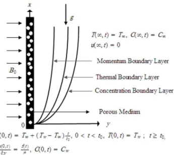
Let us consider the unsteady free convection flow of an incompressible viscous fluid over an infinite vertical plate embedded in a porous medium. The physical configuration of the problem is shown in Fig. 1. Thex-axis is taken along the plate and they-axis is taken normal to it. Initially, both the plate and fluid are at stationary conditions with the constant temperature

T? and concentrationC?. After timet~0 z

, the plate applies a time dependent shear stress f(t) to the fluid along the x-axis. Meanwhile, the temperature of the plate is raised or lowered to

T?zðTw{T?Þ t t0

when tƒt0, and thereafter, for twt0, is

maintained at constant temperature Tw and concentration is raised toCw. The radiation terms is also considered in the energy equation. However, the radiative heat flux is considered negligible inx{direction compare toy{direction. We assume that the flow is laminar and the fluid is grey absorbing-emitting radiation but no scattering medium. In addition to that we asume that the fluid is electrically conducting. Therefore, we use the following Maxwell equations

divB~0_{, Curl}E~{L B

Lt, CurlB~meJ: ð1Þ

In the above equations, B_,E and m_e are the magnetic field, electric field intensity and the magnetic permeability of the fluid, respectively. By using Ohm’s law, the current densityJis given as

J~s_ðEzV|B_Þ, ð2Þ

wheresis the electrical conductivity of the fluid. Further we make the following assumptions:

N

The quantities r,m_e and s are all constants throughout the flow field.

N

The magnetic fieldBis perpendicular to the velocity fieldV.

N

The induced magnetic fieldbis negligible compared with the imposed magnetic fieldB₀.

N

The magnetic Reynolds number is small.

N

The electric field is zero.

In view of above assumptions, the electromagnetic body force takes the linearized form [15]

1

rJ|B~

s

r½ðV|B0Þ|B0~{ sB2

0V

r : ð3Þ

Using Boussinesq’s approximation and neglecting the viscous dissipation, the equations governing the flow are given by [2,32]

Lu Lt~n

L2u

Ly2zgbTðT{T?Þzgb_CðC{C?Þ{ n Ku{

sB2 0 r u;

y,tw0,

ð4Þ

rCp

LT Lt ~k

L2T Ly2{

Lqr

Ly y,tw0, ð5Þ

LC Lt~D

L2C

Ly2 y,tw0, ð6Þ Figure 1. Physical configuration of the problem.

(3)

whereu,T,C,n,r,g,b_T,b_C,K,s,B0,Cp,k,qr, andDare the velocity of the fluid in x{direction, its temperature and concentration, the kinematic viscosity, the constant density, the gravitational acceleration, the heat transfer coefficient, the mass transfer coefficient, the permeability of the porous medium, the electric conductivity of the fluid, the applied magnetic field, the heat capacity at constant pressure, the thermal conductivity, the radiative heat flux and mass diffusivity.

The corresponding initial and boundary conditions are

u yð ,0Þ~0,T yð ,0Þ~_T?,C yð ,0Þ~C?; Vy§0,

Luð Þ0,t Ly ~

f tð Þ

m ,Cð Þ0,t ~Cw; tw0,

Tð Þ0,t ~T?zðTw{T?Þ t t0

, 0vtvt0,Tð Þ0,t~Tw; t§t0,

uð?,tÞ~0,Tð?,tÞ~T?,Cð?,tÞ~C?; tw0: ð7Þ

The radiation heat flux under Rosseland approximation for optically thick fluid [8,9,29,30,31] is given by

qr~{ 4s 3kR

LT4

Ly , ð8Þ

wheres_and_k_R_{are the Stefan-Boltzmann constant and the mean} spectral absorption coefficient respectively. It is supposed that the temperature difference within the flow are sufficiently small, then Eq. (8) can be linearized by expandingT4_{into Taylor series about} T?, and neglecting higher order terms, we find that

T4&4T3

?T{3T

4

?: ð9Þ

Substituting Eq. (9) into Eq. (8) and then putting the obtained result in Eq. (5), we get

PrLT

Lt ~nð1zNrÞ L2T

Ly2; y,tw0, ð10Þ

wherePr,nandNrare defined by

Pr~mCp k ,n~

m r,Nr~

16sT3

?

3kkR : ð

11Þ

By introducing the following dimensionless variables

u~u ffiffiffiffi t0 n r

,T~T{T? Tw{T?

,C~C{C? Cw{C?

,y~ y ffiffiffiffiffiffi nt0

p ,

t~t t0

,fð Þt ~t0 mf t0t

ð Þ, ð12Þ

into Eqs. (4), (6) and (10) and dropping out the star notations, we get

Lu Lt~

L2u

Ly2zGrTzGmC{Kpu{Mu, ð13Þ

PreffLT

Lt ~ L2T

Ly2, ð14Þ

LC Lt ~

1

Sc L2C

Ly2, ð15Þ

wherePreff~ Pr

1zNris the effective Prandtl number [29]; Eq. (10)

Gr~gbTðTw{T?Þn U3

0

,Gm~gbcðCw{C?Þn U3

0 ,

M~sB 2 0t0

r ,Sc~

n D,Kp~

nt0 K,t0~

n U2

0 ,

are the Grashof number, modified Grashof number, magnetic parameter, Schmidt number, the inverse permeability parameter for the porous medium and the characteristic time respectively.

The corresponding dimensionless initial and boundary condi-tions are

u yð ,0Þ~0,T yð ,0Þ~0C(y,0)~0; V_y§0,

Lu

LyDy~0~f tð Þ,Tð Þ0,t~t;0vtƒ1,Tð Þ0,t ~1; tw1, ð16Þ

Cð Þ0,t ~1,Cð?,tÞ~0,Tð?,tÞ~0,uð?,tÞ~0; tw0:

Solution of the Problem

In order to solve Eqs. (13)–(15) under conditions (16), we use the Laplace transform technique and get the following differential equations

quu yð ,qÞ~L 2

u u yð ,qÞ

Ly2 zGrTT yð ,qÞzGmCC yð ,qÞ

{Kpuu yð ,qÞ{Muu yð ,qÞ,

ð17Þ

T

T yð ,qÞ~ 1

Preff q

L2_T_{T y}_ð _,_q_Þ

Ly2 , ð18Þ

C

C yð ,qÞ~ 1 Scq

L2_C_{C y}_ð _,_q_Þ

Ly2 , ð19Þ

(4)

C

Cð?,qÞ~0,_C_C_ð_0,_q_Þ~1

q,TTð?,qÞ~0,

u

uð?,qÞ~0, Luu yð ,qÞ

Ly Dy~0~F qð Þ,Tð0,qÞ~

1{e{q

q2 : ð20Þ

Solving Eq. (18) in view of Eq. (20), we get

T

T yð ,qÞ~1 q2e

{y ffiffiffiffiffiffiffiffiffiffiffi_q_Pr eff

p

{e {q

q2 e

p

, ð21Þ

which upon inverse Laplace transform gives

T yð Þ,t~f yð Þ,t {f yð ,t{1ÞH tð{1Þ, ð22Þ

where

f yð Þ,t ~ Preffy 2

2 zt

erfc ffiffiffiffiffiffiffiffiffiffiffiffi Preffy p 2 ffiffi t p ! { ffiffiffiffiffiffiffiffiffiffiffi Prefft p r

yexp {Preffy 2

4t

ð23Þ

and

LT yð Þ,t Ly Dy~0~

2 ffiffiffiffiffiffiffiffiffiffi Preff p ffiffiffi p p ffiffi t p

{pffiffiffiffiffiffiffiffiffi_t{1H tð{1Þ

, ð24Þ

is the corresponding heat transfer rate also known as Nusselt number. Here erf(:) and erfc(:) denote the error function and complementary error function of Gauss [28].

Solution of Eq. (19) using boundary conditions from Eq. (20) yields

C yð ,qÞ~1 qe

{ypffiffiffiffiffiffiScq_,

ð25Þ

which upon inverse Laplace transform gives

C yð Þ,t ~erfc y ffiffiffiffiffi Sc p 2 ffiffi t p !

ð26Þ

and

LC yð Þ,t

Ly Dy~0~{ ffiffiffiffiffi Sc p

ffiffiffiffiffi pt

p , ð27Þ

is the corresponding mass transfer rate also known as Sherwood number.

The solution of Eq. (17) under boundary conditions (20) results

u

u yð ,qÞ~ a1 ffiffiffi q p

q2 _q_{_a 2

ð Þ ffiffiffiffiffiffiffiffiffiffiffiffiffiffi qzH1

p e{y ffiffiffiffiffiffiffiffiffiffi_q

zH₁

p

{ a1

ffiffiffi q p _e{q

q2 _q_{_a 2

ð Þ ffiffiffiffiffiffiffiffiffiffiffiffiffiffi qzH1

p e{y ffiffiffiffiffiffiffiffiffiffi_q_z_H 1 p

{ F qð Þ ffiffiffiffiffiffiffiffiffiffiffiffiffiffi qzH1

p e{y ffiffiffiffiffiffiffiffiffiffi_q

zH₁

p

{ a3

q2_ð_q{_a₂_Þe

p

z a3e {q

q2 _q_{_a 2

ð Þe

p

z a4

ffiffiffi q p

q qð {a5ÞpffiffiffiffiffiffiffiffiffiffiffiffiffiffiqzH1

e{y ffiffiffiffiffiffiffiffiffiffi_q_z_H 1 p

{ a6

q qð {a5Þ

e{ypffiffiffiffiffiffiqSc_,

ð28Þ

which upon inverse Laplace transform results

u yð Þ,t~_u_cð Þ_y,t z_u_mð Þ_y,t , ð29Þ

where

ucð Þy,t ~a1

ðt

0

ea₂ðt{sÞ_erf ffiffiffiffiffiffiffiffiffiffiffiffiffiffiffiffiffi a2ðt{sÞ

p

a2

ð Þ32

{2 ffiffiffiffiffiffiffiffiffi t{s

p ffiffiffi p p a2 ! e{H₁s{y

2 4s ffiffiffiffiffi

ps

p ds

z a1 a2p

ðt{1

0

2pffiffiffiffiffiffiffiffiffiffiffiffiffiffiffiffit{₁{_s

e{H1s{y

2 4s ﬃﬃ s p ds 2 6 4 3 7 5H tð{1Þ

{ a1 a2

ð Þ32 ffiffiffi

p

p ðt{1

0

ea2ðt{1{sÞ{H₁s{y

2

4serf ffiffiffiffiffiffiffiffiffiffiffiffiffiffiffiffiffiffiffiffiffiffiffiffi a2ðt{1{sÞ

p ﬃﬃ s p ds 2 6 4 3 7 5H tð{1Þ

z_a₄ ðt

0

ea₅ðt{sÞ_erf ffiffiffiffiffiffiffiffiffiffiffiffiffiffiffiffiffi a5ðt{sÞ

p

ffiffiffiffiffi a5

p {2 ffiffiffiffiffiffiffiffiffi t{s

p ffiffiffi p p _a 2 ! e{H₁s{y

2 4s ffiffiffiffiffi

ps

p ds

za3 a2

tzPreffy

2

erfc y ffiffiffiffiffiffiffiffiffiffi Preff p 2 ffiffi t p !

{a3 a2 y ffiffiffiffiffiffiffiffiffiffi Preff p ffiffi t p ffiffiffi p p e

{y2 Pr_eff

4t za3

a2 2

{a3e

a₂tzy ffiffiffiffiffiffiffiffiffiffiffiffi_Pr eff a2

p

2a2 2

erfc y ffiffiffiffiffiffiffiffiffiffi Preff p

2 ﬃﬃ t

p zpffiffiffiffiffiffia2t

!

{a3e

a₂t{y ffiffiffiffiffiffiffiffiffiffiffiffi_Pr eff a2

p

2a2 2

2 ﬃﬃ t

p { ffiffiffiffiffiffi a2t

p !

{a3 a2

t{₁

ð ÞzPreffy

2

2 ffiffiffiffiffiffiffiffiffi t{1

p !

H t_ð{₁_Þ

za3 a2

y ffiffiffiffiffiffiffiffiffiffi Preff p ffiffiffiffiffiffiffiffiffi

t{1

p

ffiffiffi

p

p e

{y2 Pr_eff

4ðt{1Þ _{H t}_ð{₁_Þ

{a3 a2 2

p !

H t_ð{1_Þza6 a5

erfc y ffiffiffiffiffi Sc p 2 ffiffi t p !

za3e

a₂ðt{1Þzy ffiffiffiffiffiffiffiffiffiffiffiffi_Pr eff a2

p

2a2 2

2pffiffiffiffiffiffiffiffiffit{1

z ffiffiffiffiffiffiffiffiffiffiffiffiffiffiffiffiffia2ðt{1Þ

p

! H t_ð{1_Þ

za3e

a₂ðt{1Þ{y ffiffiffiffiffiffiffiffiffiffiffiffi_Pr eff a2

p

2a2 2

2pffiffiffiffiffiffiffiffiffit{₁

{ ffiffiffiffiffiffiffiffiffiffiffiffiffiffiffiffiffia2ðt{1Þ

p

! H t_ð{1_Þ

{a6e

a₅t{y ffiffiffiffiffiffiffiffi_a

5Sc

p

2a5

erfc y ffiffiffiffiffi Sc

p

2 ﬃﬃ t

p {pffiffiffiffiffiffia5t

!

{a6e

a₅tzypffiffiffiffiffiffiffiffia₅Sc

2a5

erfc y ffiffiffiffiffi Sc

p

2 ﬃﬃ t

p zpffiffiffiffiffiffia5t

!

ð30Þ

and

umð Þy,t ~{ 1 ffiffiffi p p ðt 0

f tð{sÞe{H₁s{y

2 4s

ﬃﬃ s

p , ð31Þ

(5)

It is noted from Eqs. (22) and (30) thatT(y,t) is valid for all positive values ofPreff while theuc(y,t)is not valid forPreff~1. Therefore, to getuc(y,t)when the effective Prandtl number is not equal to one, we make Preff~1 into Eq. (14), use a similar procedure as discussed above, and obtain

u

u yð ,qÞ~ {a14 q32 ffiffiffiffiffiffiffiffiffiffiffiffiffiffi

qz_H₁

p e{y

ffiffiffiffiffiffiffiffiffiffi qzH₁

p

z a14e {q

q32 ffiffiffiffiffiffiffiffiffiffiffiffiffiffi qz_H₁

p e{y

ffiffiffiffiffiffiffiffiffiffi qzH₁

p

{ F qð Þ ffiffiffiffiffiffiffiffiffiffiffiffiffiffi qzH1

p e{y ffiffiffiffiffiffiffiffiffiffi_q_z_H 1 p

za14 q2e

{ypﬃﬃ_q {a14e

{q

q2 e

{ypﬃﬃ_q

z a4

ffiffiffi q p

q qð {a5ÞpffiffiffiffiffiffiffiffiffiffiffiffiffiffiqzH1

e{y ffiffiffiffiffiffiffiffiffiffi_q_z_H 1 p

{ a6

q q_ð {_a₅_Þe {ypffiffiffiffiffiffiqSc

:

ð32Þ

By taking inverse Laplace transform we find that

u yð Þ,t~{2a14 p

ðt

0 ffiffiffiffiffiffiffiffiffi t{s p

e{H₁s{y

2 4s

ﬃﬃ s

p ds

z 2a14 p

ðt{1

0

ffiffiffiffiffiffiffiffiffiffiffiffiffiffiffiffi t{1{s p

e{H₁s{y

2 4s ﬃﬃ s p ds 0 B @ 1 C AH tð{1Þ

za4 ðt

0

ea₅ðt{sÞ_erf ffiffiffiffiffiffiffiffiffiffiffiffiffiffiffiffiffi a5ðt{sÞ p

ffiffiffiffiffi a5

p {2

ffiffiffiffiffiffiffiffiffi t{_s p ffiffiffi p p a2 !

e{H1s{y

2 4s

ffiffiffiffiffi ps

p ds

za14 tz y2

2

erfc y

2 ffiffi t p {y ffiffi t p ffiffiffi p p e

{y2 4t

" #

{a6e

a₅t{ypffiffiffiffiffiffiffiffia₅Sc

2a5

erfc y ffiffiffiffiffi Sc p

2 ffiffi t p { ffiffiffiffiffiffia5t

p !

{a14 t{1z y2

2

erfc y

{y ffiffiffiffiffiffiffiffiffi t{1

p

ffiffiffi p

p e

{y2 4ðt{1Þ

" #

H tð{1Þ

za6 a5

erfc y ffiffiffiffiffi Sc p 2 ffiffi t p ! { 1 ffiffiffi p p ðt 0

f tð{sÞe{H₁s{y

2 4s

ﬃﬃ s

p ds

{a6e

a₅tzy ffiffiffiffiffiffiffiffi_a 5Sc p

2a5

2 ffiffi t p zpffiffiffiffiffiffia5t

! ,

ð33Þ

where

a1~

Gr ffiffiffiffiffiffiffiffiffiffi Preff p

Preff{1 ,a2~

H1 Preff{1,a3~

Gr

Preff{1,a4~

GmpffiffiffiffiffiSc Sc{1 ,

a5~ H1 Sc{1,a6~

Gm Sc{1,a7~

Gr ffiffiffiffiffi Pr

p

Pr{1,a8~

H1 Pr{1,

a9~ Gr

Pr{1,a10~

Kp

Preff{1,a11~

Kp

Sc{1,a12~

M

Preff{1,

a13~ M

Sc{1,a14~

Gr H1

,H1~KpzM:

ð34Þ

Plate with Constant Temperature

Equations (22) and (29) give analytical expressions for the temperature and velocity near a vertical plate with ramped temperature. In order to highlight the effect of the ramped temperature distribution of the boundary on the flow, it is important to compare such a flow with the one near a plate with constant temperature. It can be shown that the temperature, rate of heat transfer and velocity for the flow near an isothermal plate are

T yð Þ,t ~erfc y ffiffiffiffiffiffiffiffiffiffi Preff p 2 ffiffi t p !

, ð35Þ

LTð Þ0,t Ly ~{ ffiffiffiffiffiffiffiffiffiffi Preff p ffiffiffiffiffi pt

p , ð36Þ

ucð Þy,t~

a1 ffiffiffiffiffiffiffi pa2 p

ðt

0

ea2ðt{sÞ{H₁s{y

2

4s_erfpffiffiffiffiffiffiffiffiffiffiffiffiffiffiffiffiffi_a₂ð_t{sÞ

ﬃﬃ s

p ds

z a4 ffiffiffiffiffiffiffi pa5 p

ðt

0

ea5ðt{sÞ{H₁s{y

2

4s_erfpffiffiffiffiffiffiffiffiffiffiffiffiffiffiffiffiffi_a₅ð_t{sÞ

ﬃﬃ s

p ds

{ a3

2a2

ea2tzy ffiffiffiffiffiffiffiffiffiffiffiffiffi_a 2 Preff

p

2 ﬃﬃ t

p z ffiffiffiffiffiffia2t

p !

{ a3

2a2

ea2t{y ffiffiffiffiffiffiffiffiffiffiffiffiffi_a 2 Preff

p

2 ﬃﬃ t

p {pffiffiffiffiffiffi_a₂_t !

{ a6

2a5

ea5t{y ffiffiffiffiffiffiffiffi_a 5Sc p

2 ffiffi t p {pffiffiffiffiffiffia5t

!

za3 a2

za6 a5

{ a6

2a5

ea5tzy ffiffiffiffiffiffiffiffi_a 5Sc p

! ,

umð Þy,t~{ 1 ffiffiffi p p ðt 0

f tð{sÞe{H₁s{y

2 4s

ﬃﬃ s

p ds:

ð37Þ

As previously, Eq. (37) is not valid forPreff~1. Therefore we calculate separately solution for velocity by takingPreff~1into Eq. (14) and finally get

u yð Þ,t ~a14 erfc y

2 ﬃﬃ t p

{a14 ffiffiffi p p

ðt

0 e{H₁s{y

2 4s

ffiffiffiffiffiffiffiffiffiffiffiffiffiffi t{s ð Þs

p ds

ðt

0

ea5ðt{sÞ{H₁s{y

2

4serf ffiffiffiffiffiffiffiffiffiffiffiffiffiffiffiffiffi a5ðt{sÞ p

ﬃﬃ s

p ds

za6 a5

erfc y ffiffiffiffiffi Sc p 2 ffiffi t p ! { 1 ffiffiffi p p ðt 0

f tð{sÞe{H₁s{y2

4s

ﬃﬃ s

p ds

{ a6

2a5

2 ffiffi t p zpffiffiffiffiffiffi_a₅_t

!

{ a6

2a5

p !

:

(6)

Limiting Cases

In this section we discuss few limiting cases of our general solutions.

5.1 Solution in the absence of porous effects for ramped and constant wall temperature (Kp?0)

u yð Þ,t~a1 ðt

0

ea₁₂ðt{sÞ_erf ffiffiffiffiffiffiffiffiffiffiffiffiffiffiffiffiffiffi a12ðt{sÞ p

a12 ð Þ32

{2 ffiffiffiffiffiffiffiffiffi t{s p ffiffiffi p p a12 !

e{Ms{y

2 4s

ffiffiffiffiffi ps

p ds

z a1 a12p

ðt{1

0

2pffiffiffiffiffiffiffiffiffiffiffiffiffiffiffiffit{1{s

e{Ms{y 2 4s ﬃﬃ s p ds 2 6 4 3 7 5H tð{1Þ

{ a1

a12 ð Þ32 ffiffiffi

p p

ðt{1

0

ea12ðt{1{sÞ{Ms{y

2

4s_erfpffiffiffiffiffiffiffiffiffiffiffiffiffiffiffiffiffiffiffiffiffiffiffiffiffiffi_a₁₂ð_t{1{sÞ

ﬃﬃ s p ds 2 6 4 3 7 5H tð{1Þ

z_a₄ ðt

0

ea₁₃ðt{sÞ_erf ffiffiffiffiffiffiffiffiffiffiffiffiffiffiffiffiffiffi a13ðt{sÞ p

ffiffiffiffiffiffiffi a13

p {2

ffiffiffiffiffiffiffiffiffi t{s p ffiffiffi p p a12 !

e{Ms{y

2 4s

ffiffiffiffiffi ps

p ds

za3 a12

tzPreffy 2

2

erfc y ffiffiffiffiffiffiffiffiffiffi Preff p 2 ffiffi t p ! { 1 ffiffiffi p p ðt 0

f tð{sÞe{Ms{y

2 4s

ﬃﬃ s

p ds

{a3 a12 y ffiffiffiffiffiffiffiffiffiffi Preff p ffiffi t p ffiffiffi p p e

{y2 Pr_eff 4t za3

a2 12

{a3e

a₁₂tzy ffiffiffiffiffiffiffiffiffiffiffiffiffiffi_Pr eff a12 p

2a2 12

2 ﬃﬃ t

p zpffiffiffiffiffiffiffiffia12t !

{a3e

a₁₂t{y ffiffiffiffiffiffiffiffiffiffiffiffiffiffi_Pr eff a12 p

2a2 12

2 ﬃﬃ t

p { ffiffiffiffiffiffiffiffia12t

p !

{a3 a12

t{₁

ð ÞzPreffy 2

2

2pffiffiffiffiffiffiffiffiffit{₁ !

H t_ð{₁_Þ

za3 a12

t{1

p

ffiffiffi p

p e

{y2 Pr_eff 4ðt{1Þ _{H t}_ð{₁_Þ

{a6e

a₁₃t{y ffiffiffiffiffiffiffiffiffi_a 13Sc p

2a13

2 ﬃﬃ t

p !

{a3 a2 12

H tð{1Þza6 a13

za3e

a₁₂ðt{1Þzy ffiffiffiffiffiffiffiffiffiffiffiffiffiffi_Pr eff a12 p

2a2 12

p z ffiffiffiffiffiffiffiffiffiffiffiffiffiffiffiffiffiffiffia12ðt{1Þ p

! H tð{1Þ

za3e

a₁₂ðt{1Þ{y ffiffiffiffiffiffiffiffiffiffiffiffiffiffi_Pr eff a12 p

2a2 12

p { ffiffiffiffiffiffiffiffiffiffiffiffiffiffiffiffiffiffiffia12ðt{1Þ p

! H tð{1Þ

{a6e

a₁₃tzy ffiffiffiffiffiffiffiffiffi_a 13Sc p

2a13

2 ﬃﬃ t

p z ffiffiffiffiffiffiffiffia13t

p !

,

ð39Þ

u yð Þ,t ~ a1 ffiffiffiffiffiffiffiffiffi pa12 p

ðt

0

ea12ðt{sÞ{Ms{y

2

4serf ffiffiffiffiffiffiffiffiffiffiffiffiffiffiffiffiffiffi a12ðt{sÞ p

ﬃﬃ s

p ds

z a4 ffiffiffiffiffiffiffiffiffi pa13 p

ðt

0

ea13ðt{sÞ{Ms{y

2

4s_erfpffiffiffiffiffiffiffiffiffiffiffiffiffiffiffiffiffiffi_a₁₃ð_t{sÞ

ﬃﬃ s

p ds

{ a6

2a13

ea13t{ypffiffiffiffiffiffiffiffiffia₁₃Sc_erf_c y ffiffiffiffiffi Sc p

2 ﬃﬃ t

p !

{ a3

2a12

ea12tzy ffiffiffiffiffiffiffiffiffiffiffiffiffiffi_a 12 Preff

p

2 ﬃﬃ t

{ a3

2a12

ea12t{y ffiffiffiffiffiffiffiffiffiffiffiffiffiffi_a 12 Preff

p

2 ﬃﬃ t

p !

za3 a12

za6 a13

{ a6

2a13

ea13tzy ffiffiffiffiffiffiffiffiffi_a 13Sc p

2 ﬃﬃ t

p !

:

ð40Þ

5.2 Solution in the absence of thermal radiation (Nr?₀₎ In the absence of thermal radiation, the corresponding solutions for ramped and constant wall temperature are directly obtained from the general solutions (22), (24), (29) and (35)–(37) by taking

Nr?₀_{and replacing}_Preff _by_Pr_i :e:

u yð Þ,t ~a7 ðt

0

ea₈ðt{sÞ_erf ffiffiffiffiffiffiffiffiffiffiffiffiffiffiffiffiffi a8ðt{sÞ p

a8 ð Þ32

{2 ffiffiffiffiffiffiffiffiffi t{s p ffiffiffi p p a8 !

e{H1s{y

2 4s

ffiffiffiffiffi ps

p ds

z a7 pa8

ðt{1

0

2 ffiffiffiffiffiffiffiffiffiffiffiffiffiffiffiffi t{1{s p

e{H₁s{y

2 4s ﬃﬃ s p ds 2 6 4 3 7 5H tð{1Þ

{ a7

a8 ð Þ32 ffiffiffi

p p

ðt{1

0

erf ffiffiffiffiffiffiffiffiffiffiffiffiffiffiffiffiffiffiffiffiffiffiffiffia8ðt{1{sÞ p

ea8ðt{1{sÞ{H₁s{y

2 4s ﬃﬃ s p ds 2 6 4 3 7 5H tð{1Þ

za4 ðt

0

ea₅ðt{sÞ_erf ffiffiffiffiffiffiffiffiffiffiffiffiffiffiffiffiffi a5ðt{sÞ p

ffiffiffiffiffi a5

p {2

ffiffiffiffiffiffiffiffiffi t{s p ffiffiffi p p a8 !

e{H₁s{y

2 4s

ffiffiffiffiffi ps

p ds

za9 a8

tzPry 2

2

erfc y ffiffiffiffiffi Pr p 2 ffiffi t p ! { 1 ffiffiffi p p ðt 0

f tð{sÞe{H₁s{y

2 4s

ﬃﬃ s

p ds

{a9 a8

ypffiffiffiffiffiPr ffiffi t p

ffiffiffi p

p e

{y2 Pr 4t za9

a2 8

erfc y ffiffiffiffiffi Pr p 2 ffiffi t p !

{a9e

a₈tzy ffiffiffiffiffiffiffiffi_Pr_a 8 p

2a2 8

erfc y ffiffiffiffiffi Pr

p

!

{a9e

a₈t{y ffiffiffiffiffiffiffiffi_Pr_a 8 p

2a2 8

p

!

(7)

{a9 a8

t{1

ð ÞzPry 2

2

p

H tð{1Þ

{a9 a8

p

p !

H tð{1Þza9 a8

y ffiffiffiffiffi Pr

p ffiffiffiffiffiffiffiffiffi t{1

p

ffiffiffi p

p e

{y2 Pr 4ðt{1Þ_{H t}ð{1Þ

za9e

a₈ðt{1Þzy ffiffiffiffiffiffiffiffi_Pr_a 8 p

2a2 8

p

2pffiffiffiffiffiffiffiffiffit{1z

ffiffiffiffiffiffiffiffiffiffiffiffiffiffiffiffiffi a8ðt{1Þ p

! H tð{1Þ

za9e

a₁₂ðt{1Þ{y ffiffiffiffiffiffiffiffiffiffi_Pr_a 12 p

2a2 8

p

{ ffiffiffiffiffiffiffiffiffiffiffiffiffiffiffiffiffia8ðt{1Þ p

! H tð{1Þ

{a6e

a₅tzy ffiffiffiffiffiffiffiffi_a 5Sc p

2a5

!

za6 a5

2 ﬃﬃ t p

!

{a6e

a₅t{ypffiffiffiffiffiffiffiffia₅Sc

2a5

p !

,

T yð Þ,t ~f1ð Þy,t {f1ðy,t{1ÞH tð{1Þ, ð42Þ

where

f1ð Þy,t ~ Pry2

2 zt

erfc ffiffiffiffiffiffi Pr

p y

2 ﬃﬃ t p

!

{ ffiffiffiffiffiffiffiffi Prt p r

yexp {Pry 2

4t

ð43Þ

and

LT yð Þ,t Ly Dy~0~

2pffiffiffiffiffiPr ffiffiffi p

p ﬃﬃ

t p

{pffiffiffiffiffiffiffiffiffit{1H tð{1Þ

: ð44Þ

u yð Þ,t ~ a7 ffiffiffiffiffiffiffi pa8 p

ðt

0

ea8ðt{sÞ{H₁s{y

2

4serf ffiffiffiffiffiffiffiffiffiffiffiffiffiffiffiffiffi a8ðt{sÞ p

ﬃﬃ s

p ds

ðt

0

ea5ðt{sÞ{H₁s{y2

4s_erfpffiffiffiffiffiffiffiffiffiffiffiffiffiffiffiffiffi_a₅ð_t{sÞ

ﬃﬃ s

p ds

{ a9

2a8

ea8tzypffiffiffiffiffiffiffiffia_{8 Pr}_erf_c y ffiffiffiffiffi Pr

p

2 ffiffi t p z ffiffiffiffiffiffia8t

p !

{ a9

2a8

ea8t{y ffiffiffiffiffiffiffiffi_a 8 Pr p

p

!

za9 a8

p

2 ﬃﬃ t p

!

za6 a5

2 ﬃﬃ t p

!

{ a6

2a5

!

{ a6

2a5

p !

{ 1

ffiffiffi p p

ðt

0

f tð{sÞe{H₁s{y2

4s

ﬃﬃ s

p ds,

ð45Þ

T yð Þ,t ~erfc y ffiffiffiffiffi Pr

p

2 ﬃﬃ t p

!

, ð46Þ

Figure 2. Velocity profiles for different values ofGrwhen the plate applies a constant shear stressf~{0_:25.

doi:10.1371/journal.pone.0090280.g002

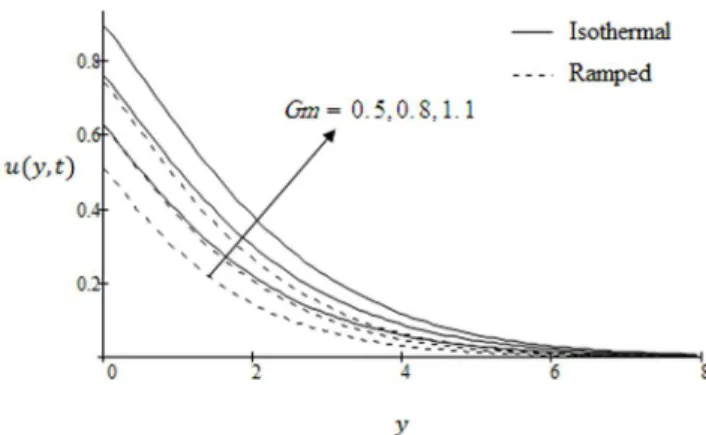
Figure 3. Velocity profiles for different values ofGmwhen the plate applies a constant shear stressf~{0_:25.

Figure 4. Velocity profiles for different values ofScwhen the plate applies a constant shear stressf~{0_:25.

(8)

LTð Þ0,t Ly ~{

ffiffiffiffiffi Pr

p

ffiffiffiffiffi pt

p : ð47Þ

5.3 Solutions in the absence of free convection

Let us assume that the flow is caused only due to bounding plate and the corresponding buoyancy forces are zero equivalently it shows the absence of free convection due to the differences in temperature and mass gradients i.e. the termsGrandGmare zero. This shows that the convective parts of velocities are zero in both cases of ramped wall and constant temperature and the flow is only governed by the mechanical part of velocities given by Eqs. (31) and (37).

5.4 Solutions in the absence of mechanical effects In this case we assume that the infinite plate is in static position at every time i.e. the functionf(t)is zero for all values oftand the mechanical parts for both ramped and constant wall temperature are equivalently zero. In such a situation, the motion in the fluid is induced only due to the free convection which causes due to the buoyancy forces. Therefore, the velocities of the fluid in both cases of ramped and constant wall temperature are only represented by their convective parts given by Eqs. (30) and (37).

5.5 Solution in the absence of magnetic parameter (M?₀₎

As it is clear from Eqs. (22) and (26) that the temperature and concentration distributions are not effected by the magnetic parameterM, and the velocities withM~0for both ramped and constant wall temperature are given by

u yð Þ,t ~a1 ðt

0

ea₁₀ðt{sÞ_erf ffiffiffiffiffiffiffiffiffiffiffiffiffiffiffiffiffiffi a10ðt{sÞ p

a10 ð Þ32

{2 ffiffiffiffiffiffiffiffiffi t{s p

ffiffiffi p p

a10 !

e{Kps{y

2 4s

ffiffiffiffiffi ps

p ds

z a1 pa10

ðt{1

0

2pffiffiffiffiffiffiffiffiffiffiffiffiffiffiffiffit{1{se{Kps{y

2 4s

ﬃﬃ s

p ds

2

6 4

3

7 5H tð{1Þ

{ a1

a10 ð Þ32pffiffiffi_p

ðt{1

0

erf ffiffiffiffiffiffiffiffiffiffiffiffiffiffiffiffiffiffiffiffiffiffiffiffiffiffi a10ðt{1{sÞ p

ea10ðt{1{sÞ{_Kps{y

2 4s

ﬃﬃ s

p ds

2

6 4

3

7 5Hðt{1Þ

za4 ðt

0

ea₁₁ðt{sÞ_erf ffiffiffiffiffiffiffiffiffiffiffiffiffiffiffiffiffiffi a11ðt{sÞ p

ffiffiffiffiffiffiffi a11

p {2

ffiffiffiffiffiffiffiffiffi t{s p

ffiffiffi p p

a10 !

e{Kps{y 2 4s

ffiffiffiffiffi ps

p ds

za3 a10

tzPreffy 2

2

2 ﬃﬃ t p

!

{a3 a10

y ffiffiffiffiffiffiffiffiffiffi Preff

p ﬃﬃ

t p

ffiffiffi p

p e

{y2 Pr_eff 4t za3

a2 10

2 ﬃﬃ t p

!

{ 1

ffiffiffi p p

ðt

0

f tð{sÞe{_Kps{y

2 4s

ﬃﬃ s

p ds

{a3e

a₁₀tzy ffiffiffiffiffiffiffiffiffiffiffiffiffiffi_Pr eff a10 p

2a2 10

2 ﬃﬃ t

p !

{a3e

a₁₀t{y ffiffiffiffiffiffiffiffiffiffiffiffiffiffi_Pr eff a10 p

2a2 10

2 ﬃﬃ t

p !

{a3 a10

t{1

ð ÞzPreffy 2

2

p !

H tð{1Þ

za3 a10

t{1

p

ffiffiffi p

p e

{y2 Pr_eff

4ðt{1Þ _{H t}ð{1Þ

{a6e

a₁₁t{ypffiffiffiffiffiffiffiffiffia₁₁Sc

2a11

2 ﬃﬃ t

p !

{a3 a2

10 erfc y

ffiffiffiffiffiffiffiffiffiffi Preff p

p !

H tð{1Þza6 a11

2 ﬃﬃ t p

!

za3e

a₁₀ðt{1Þzy ffiffiffiffiffiffiffiffiffiffiffiffiffiffi_Pr eff a10 p

2a2 10

p z ffiffiffiffiffiffiffiffiffiffiffiffiffiffiffiffiffiffiffia10ðt{1Þ p

! H tð{1Þ

za3e

a₁₀ðt{1Þ{y ffiffiffiffiffiffiffiffiffiffiffiffiffiffi_Pr eff a10 p

2a2 10

2pffiffiffiffiffiffiffiffiffit{1{

ffiffiffiffiffiffiffiffiffiffiffiffiffiffiffiffiffiffiffi a10ðt{1Þ p

! H tð{1Þ

{a6e

a₁₁tzy ffiffiffiffiffiffiffiffiffi_a 11Sc p

2a11

2 ﬃﬃ t

,

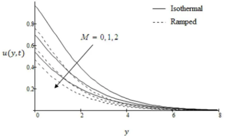
ð48Þ Figure 5. Velocity profiles for different values ofM when the

plate applies a constant shear stressf~{0_:25.

Figure 6. Velocity profiles for different values oft when the plate applies a constant shear stressf~{0

(9)

u yð Þ,t ~ a1 ffiffiffiffiffiffiffiffiffi pa10 p

ðt

0

ea10ðt{sÞ{_Kps{y

2

ﬃﬃ s

p ds

z a4 ffiffiffiffiffiffiffiffiffi pa11 p

ðt

0

ea11ðt{sÞ{_Kps{y

2

ﬃﬃ s

p ds

{ a3

2a10

ea10tzy ffiffiffiffiffiffiffiffiffiffiffiffiffiffi_a 10 Preff

p

2 ﬃﬃ t

p zpffiffiffiffiffiffiffiffi_a₁₀_t !

{ a3

2a10

ea10t{y ffiffiffiffiffiffiffiffiffiffiffiffiffiffi_a 10 Preff

p

2 ﬃﬃ t

p {pffiffiffiffiffiffiffiffia10t !

za3 a10

2 ﬃﬃ t p

!

za6 a11

2 ﬃﬃ t p

!

{ a6

2a11

ea11tzy ffiffiffiffiffiffiffiffiffi_a 11Sc p

2 ﬃﬃ t

{ 1

ffiffiffi p p

ðt

0

f tð{sÞe{Kps{y

2 4s

ﬃﬃ s

p ds

{ a6

2a11

ea11t{y ffiffiffiffiffiffiffiffiffi_a 11Sc p

2 ﬃﬃ t

p {pffiffiffiffiffiffiffiffi_a₁₁_t !

:

ð49Þ

Special Cases

As we noted that the solutions for velocity obtained in Section 3, are more general. Therefore, we want to discuss some special cases of the present solutions together with some limiting solutions in order to know more about the physical insight of the problem. Hence, we discuss the following important special cases in the case of ramped wall temperature whose technical relevance is well-known in the literature. Similarly we can discuss some special cases of constant wall temperature solutions.

6.1 Case-I:f(t)~fH(t)

In this first case we take the arbitrary function f(t)~fH(t), wheref is a dimensionless constant andH(:)denotes the unit step function. After time t~0, the infinite vertical plate applies a constant shear stress to the fluid. The convective part of the velocity remains unchanged while the mechanical part takes the following form

umð Þy,t ~{

f ffiffiffi p p

ðt

0 e{y

2 4s{H1s

ﬃﬃ s

p ds, ð50Þ

equivalently

umð Þy,t~{

f ffiffiffiffiffiffi H1 p e{y ffiffiffiffiffi_H

1 p

z2f ffiffiffi p p

ð?

ﬃﬃ t p e

{y

2

4z2{H1z2_dz_, ð51Þ

forKp=0,M=0. Moreover, if we takeM~0, Eq. (50) reduces to the form

umð Þy,t ~{

f ffiffiffiffiffiffi Kp

p e

{y ffiffiffiffiffi Kp

p z2f

ffiffiffi p p

ð?

ﬃﬃ t pe

{y

2

4z2{Kpz 2

dz, ð52Þ

which is equivalent to [28]; Eq. (28) with the correction of ffiffiffiffiffiffi Kp p

. Furthermore, in the absence of bothKp~0andM~0, Eq. (50) is identical with [27]; Eq. (23)

umð Þy,t ~{

f ffiffiffi p p

ðt

0 e{y

2 4s

ﬃﬃ s

p ds: ð53Þ

6.2 Case-II:f(t)~fsin(vt)

In the second case, we take the arbitrary function of the form

f(t)~f sin(vt)in which the plate applies an oscillating shear stress to the fluid. Herevdenotes the dimensionless frequency of the shear stress. As previously, the convective part of velocity remains the same whereas the mechanical part takes the form

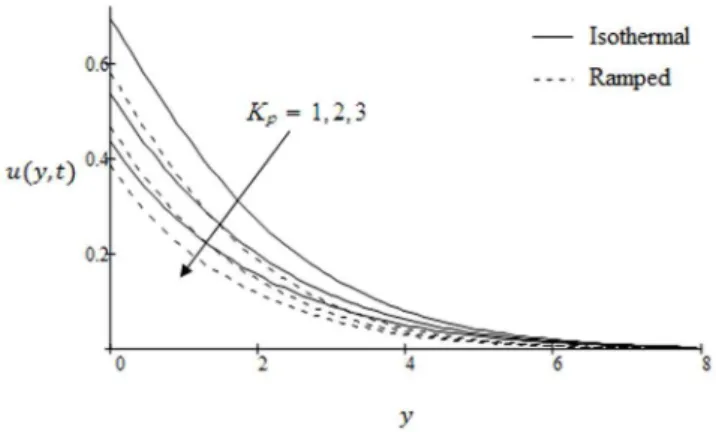
Figure 7. Velocity profiles for different values ofKp when the

Figure 8. Velocity profiles for different values of constant shear stressf.

(10)

umð Þy,t ~{

f ffiffiffi p p

ðt

0

sinðvt{vsÞe{y2

4s{H1s ﬃﬃ

s

p ds: ð54Þ

It can be further written as a sum of the steady-state and transient solutions

umð Þy,t ~umsð Þy,t zumtð Þy,t, ð55Þ

where

umsð Þy,t ~{

f ffiffiffi p p

ðt

0

sinðvt{vsÞe{y

2 4s{H1s ﬃﬃ

s

p ds, ð56Þ

umtð Þy,t~

f ffiffiffi p p

ð?

t

sinðvt{vsÞe{y

2 4s{H1s ﬃﬃ

s

p ds: ð57Þ

By takingM~0, the steady-state component reduces to [28]; Eq. (35)

umsð Þy,t ~{

f ffiffiffi p p

ðt

0

sinðvt{vsÞe{y

2 4s{Kps ﬃﬃ

s

p ds: ð58Þ

In addition when Kp~0, physically it corresponds to the absence of porous effects and Eq. (58) results in

umsð Þy,t ~{

f ffiffiffi p p

ðt

0

sinðvt{vsÞe{y

2 4s

ﬃﬃ s

p ds, ð59Þ

which can be written in simplified form as

umsð Þy,t~

f ffiffiffiffi v

p exp {y ffiffiffiffi v

2 r

cos vt{y ffiffiffiffi v

2 r

zp

4

, ð60Þ

equivalent to [27]; Eq. (33).

6.3 Case-III:f(t)~fta(aw0)

In the final case, we takef(t)~fta_{, in which the plate applies an} accelerating shear stress to the fluid where the mechanical part takes the following form

umð Þy,t~{

f ffiffiffi p p

ðt

0 t{s ð Þae{y

2 4s{H1s ﬃﬃ s

p ds: ð61Þ

The corresponding solution forM~0, namely

umð Þy,t ~{

f ffiffiffi p p

ðt

0 t{_s ð Þae{y

2 4s{Kps ﬃﬃ s

p ds, ð62Þ

is identical with [28]; Eq. (32).

Additionally, if we takeKp~0, Eq. (62) yields

umð Þy,t ~{

f ffiffiffi p p

ðt

0 t{s ð Þae{y

2 4s

ﬃﬃ s

p ds: ð63Þ

Figure 9. Velocity profiles for different values ofPreff when the

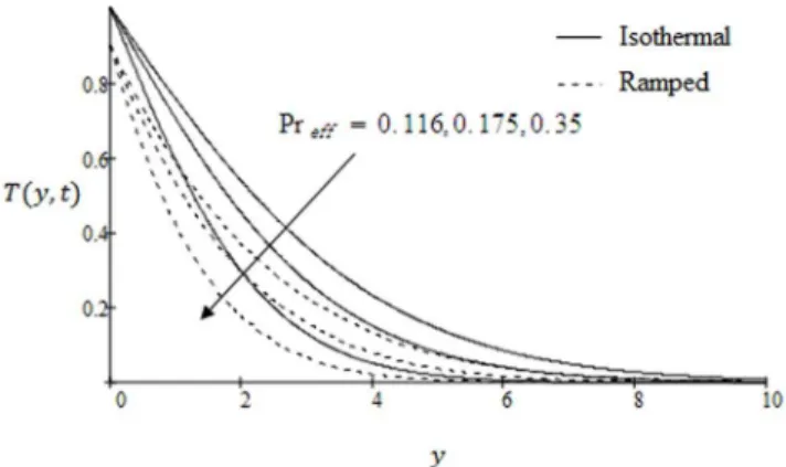
Figure 10. Temperature profile for different values ofPreff. doi:10.1371/journal.pone.0090280.g010

Figure 11. Temperature profiles for different values oft.

(11)

Results and Discussion

In order to understand the physical aspects of the problem, the numerical results for velocity, temperature and concentration are computed and plotted for various parameters of interest such as magnetic parameterM, porosity parameterKp, effective Prandtl number Preff, Grashof number Gr, modified Grashof number

Gm, dimensionless timet, Schmidt numberScand shear stressf. The graphs for velocity are shown in Figs. 2–9 where t~1:2 corresponds to isothermal velocity and t~0:9 is for ramped velocity. Figs. 10 and 11 are plotted to show the temperature variations for two types of boundary conditions namely ramped and constant wall temperatures. Furthermore, Figs. 12 and 13 are displayed to show variations in fluid concentration. Fig. 2 illustrate the influence of Grashof numberGron the velocity. It is observed that velocity increases with increasing Gr. This implies that thermal buoyancy force tends to accelerate velocity for both ramped temperature and isothermal plates. In Fig. 3 the velocity profiles for different values modified Grashof number Gm are shown. It is found that velocity increases on increasing Gmfor both ramped temperature and isothermal plate. Further, it can be observed that the velocity and boundary layer thickness decrease along y with increasing distance from the the leading edge. Moreover, we observed that the amplitude of velocity in case of isothermal plate is greater and converges slowly as compare to ramped velocity. In Fig. 4 the velocity profiles are shown for different values of Schmidt number Sc. It is observed that the velocity decreases with increasing Schmidt number. The velocity profiles for different values of magnetic parameterMare shown in Fig. 5. The range of magnetic field is taken from0to2. It is found that the velocity is decreasing with increasing values ofM in both cases of ramped and isothermal plates. Physically, it is true due to the fact that increasing values ofM causes the frictional force to increase which tends to resist the fluid flow and thus reducing its velocity. It is further observed that when the magnetic field imposed on the flow is zero (M~0), the MHD effect vanishes and the flow is termed as hydrodynamic flow.

Fig. 6 are plotted to see the difference between the ramped and isothermal plate velocities. The values oftv1correspond to ramp velocity whereastw1is for isothermal plate. It is found that ramp velocity is less than isothermal plate and converges faster. Further velocity in both cases increases with increasing time. The effects of inverse permeability parameter Kp on the velocity profiles are presented in Fig. 7. It is found that velocity decreases with increasing Kp in both cases of ramp and isothermal plate.

Physically, it is due to the fact that increasing permeability of the porous medium increases the resistance and consequently velocity decreases. This observation is an excellent agreement with the previous study [28]; Fig. 3. The effects of the shear stressf induced by the bounding plate on the non-dimensional velocity profiles are shown in Fig. 8. The velocity of fluid is found to decrease with increasingf in both cases of ramped velocity and isothermal plate. Graphical results to show the influence of the effective Prandtl number Preff on velocity profiles are presented in Fig. 9. It is observed that the velocity is a decreasing function with respect to Preff. These graphical results are in accordance with [28]; Fig. 2. The temperature variations against y for various values of effective Prandtl number are highlighted in Fig. 10. The significant decrease of the temperature is found as a result of an increase of the effective Prandtl number. The fluid temperature decreases from maximum at the boundary to a minimum value as far from the plate in both cases of ramped and constant temperature. In Fig. 11 we have shown the temperature variations for two types of boundary conditions ramped and constant plate temperatures. It is noted that the fluid temperature is greater in the case of isothermal plate than in the case of ramped temperature at the plate. This should be expected since in the latter case, the heating of the fluid takes place more gradually than in the isothermal case [18]. Moreover, with increasing time, the temperature is found to increase in both cases of ramped and constant wall temperature. The concentration profiles for different values of Schmidt number

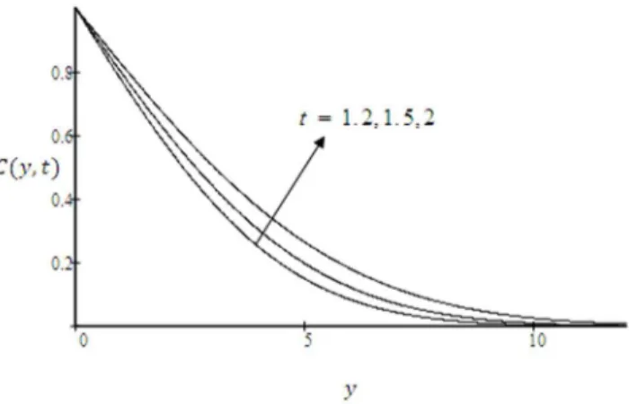
Sc, are shown in Fig. 12. It is clear from this figure that the concentration profiles and the concentration boundary layer thickness decrease with increasing values ofSc. Physically, it is true, since increase ofScmeans decrease of molecular diffusivity which results in a decrease of concentration boundary layer. The concentration profiles for different values of timetare presented in Fig. 13. It is observed that concentration profiles increase with increasingt.

Conclusions

The purpose of this work was to analyze the unsteady MHD free convection flow of an incompressible viscous fluid over an infinite plate with ramped wall temperature and applies an arbitrary shear stress to the fluid. Exact solutions for velocity, temperature (for both cases of ramped and constant wall temperature) and concentration are obtained using the Laplace transform technique and expressed in terms of the complementary error function. They satisfy all imposed initial and boundary

Figure 12. Concentration profiles for t~1

:2 and different

values ofSc.

Figure 13. Concentration profiles for Sc~0_:2 and different values oft.

(12)

conditions. These solutions are plotted in various figures for different parameters of interest. It is found that velocity of the fluid

u yð Þ,t can be written as a sum of its mechanical and thermal componentsumð Þy,t , respectivelyutð Þy,t. For the velocity solution in which the plate applies an oscillating shear stress to the fluid

f(t)~fsin(vt), the mechanical part can be further written as a sum of the steady-state and transient solutions umsð Þy,t, respec-tivelyumtð Þy,t. The thermal boundary layer thickness in case of ramped wall temperature is less than isothermal wall temperature. Magnetic parameterM retards whereas the inverse permeability parameterKp enhances the fluid motion. The thermal boundary

layer, as well as the temperature of the fluid, increases in time and decreases with respect to the effective Prandtl number Preff. The concentration boundary layer thickness decreases with increasing values ofScwhereas increases with increasingt.

Author Contributions

Conceived and designed the experiments: IK. Performed the experiments: AK. Analyzed the data: Su. Contributed reagents/materials/analysis tools: SS. Wrote the paper: FA.

References

1. Khan I, Ali F, Sharidan S, Norzieha M (2011) Effects of Hall current and mass transfer on the unsteady magnetohydrodynamic flow in a porous channel. J Phys Soc Jpn 80: 064401.

2. Das K, Jana S (2010) Heat and mass transfer effects on unsteady MHD free convection flow near a moving vertical plate in porous medium. Bull Soc Math Banja Luka 17: 15–32.

3. Das SS, Satapathy A, Das JK, Panda JP (2009) Mass transfer effects on MHD flow and heat transfer past a vertical porous plate through a porous medium under oscillatory suction and heat source. Int J Heat Mass Transfer 52: 5962– 5969.

4. Chandrakala P (2011) Radiation effects on flow past an impulsively started vertical oscillating plate with uniform heat flux. Int J Dyn Fluids 7: 1–8. 5. Das SS, Parija S, Padhy RK, Sahu M (2012) Natural convection unsteady

magneto-hydrodynamic mass transfer flow past an infinite vertical porous plate in presence of suction and heat sink. Int J Energy Environ 3: 209–222. 6. Das SS, Maity M, Das JK (2012) Unsteady hydromagnetic convective flow past

an infinite vertical porous flat plate in a porous medium, Int J Energy Environ 3: 109–118.

7. Narahari M, Ishaq A (2011) Radiation effects on free convection flow near a moving vertical plate with Newtonian heatin. J Appl Sci 11: 1096–1104. 8. Narahari M, Nayan MY (2011) Free convection flow past an impulsively started

infinite vertical plate with Newtonian heating in the presence of thermal radiation and mass diffusion. Turkish J Eng Env Sci 35: 187–198.

9. Hussanan A, Khan I, Sharidan S (2013) An exact analysis of heat and mass transfer past a vertical plate with Newtonian heating. J Appl Math Article ID 434571 http://dx.doi.org/10.1155/2013/434571.

10. Das SS, Biswal SR, Tripathy UK, Das P (2011) Mass transfer effects on unsteady hydromagnetic convective flow past a vertical porous plate in a porous medium with heat source. J Appl Fluid Mech 4: 91–100.

11. Toki CJ, Tokis JN (2007) Exact solutions for the unsteady free convection flows on a porous plate with time-dependent heating. ZAMM Z Angew Math Mech 87: 4–13.

12. Senapati N, Dhal RK, Das TK (2012) Effects of chemical reaction on free convection MHD flow through porous medium bounded by vertical surface with slip flow region. Amer J Comput Appl Math 2: 124–135.

13. Khan I, Fakhar K, Sharidan S (2011) Magnetohydrodynamic free convection flow past an oscillating plate embedded in a porous medium. J Phys Soc Jpn 80: 104401.

14. Shercliff JA (1965) Textbook of magnetohydrodynamics. London: pergamon press.

15. Hayat T, Khan I, Ellahi R, Fetecau C (2008) Some MHD flows of a second grade fluid through the porous medium. J Porous Media 11: 389–400. 16. Jha BK, Apere CA (2010) Combined effect of hall and ion-slip currents on

unsteady mhd couette flows in a rotating system. J Phys Soc Jpn 79:104401. 17. Fetecau C, Vieru D, Corina Fetecau, Akhter S (2013) General solutions for

magnetohy-drodynamic natural convection flow with radiative heat transfer and

slip condition over a moving plat. Z Naturforsch 68a 659–667 / DOI: 10.5560/ ZNA.2013-0041.

18. Chandran P, Sacheti NC, Singh AK (2005) Natural convection near a vertical plate with ramped wall temperature. Heat Mass Transf 41: 459–464. 19. Narahari M, Beg OA, Ghosh SK (2011) Mathematical modelling of mass

transfer and free convection current effects on unsteady viscous flow with ramped wall temperature. World J Mech 1: 176–184.

20. Rajesh V (2011) Chemical reaction and radiation effects on the transient MHD free convection flow of dissipative fluid past an inflnite vertical porous plate with ramped wall temperature. Chem Ind Chem Eng Quar 17: 189–198. 21. Patra1 RR, Das S, Jana RN, Ghosh SK (2012) Transient approach to radiative

heat transfer free convection flow with ramped wall temperature. J Appl Fluid Mech: 59–13.

22. Seth GS, Mahatoo GK, Sarkar S (2013) Effects of Hall current and rotation on MHD natural convection flow past an impulsively moving vertical plate with ramped temper-ature in the presence of thermal diffusion with heat absorption. Int J Energy Tech 5: 1–12.

23. Samiulhaq, Khan I, Ali F, Sharidan S (2012) MHD free convection flow in a porous medium with thermal diffusion and ramped wall temperature. J Phys Soc Jpn 81: 044401.

24. Ghara N, Das S, Maji SL, Jana RN (2012) Effect of radiation on MHD free convection flow past an impulsively moving vertical plate with ramped wall temperature. Am J Sci Ind Res 3: 376–386.

25. Das S, Mandal C, Jana RN (2012) Effects of radiation on unsteady Couette flow between two vertical parallel plates with ramped wall temperature. Int J Comput Appl 39: 37–45.

26. Navier CLMH (1827) Sur les lois dee mouvement des fluids. Mem Acad R Sci Inst Fr 6: 389–440.

27. Fetecau C, Corina Fetecau, Rana M (2011) General solutions for the unsteady flow of second-grade fluids over an inflnite plate that applies arbitrary shear to the fluid. Z Naturfors Sect A-J Phys Sci 66: 753–759.

28. Corina Fetecau, Rana M, Fetecau C (2013) Radiative and porous effects on free con-vection flow near a vertical plate that applies shear stress to the fluid. Z Naturfors Sect A-J Phys Sci 68: 130–138.

29. Magyari E, Pantokratoras A (2011) Note on the effect of thermal radiation in the linearized Rosseland approximation on the heat transfer characteristics of various boundary layer flows. Int Commun Heat Mass Transf 38: 554–556. 30. Narahari M, Dutta BK (2012) Effects of thermal radiation and mass diffusion on

free convection flow near a vertical plate with Newtonian heating. Chem Eng Commun 199: 628–643.

31. Ghosh SK, Beg OA (2008) Theoretical analysis of radiative effects on transient free convection heat transfer past a hot vertical surface in porous media. Nonlin Anal Model Control 13: 419–432.