Unsteady Free Convection Fluid Flow over an Inclined Plate in the Presence of a Magnetic Field with Thermally Stratified High Porosity Medium

J_{ournal of} A_pplied F_luid M_{echanics, Vol. 9, No. 3, pp. 1467-1475, 2016.} Available online at www.jafmonline.net, ISSN 1735-3572, EISSN 1735-3645.

Unsteady Free Convection Fluid Flow over an Inclined

Plate in the Presence of a Magnetic Field with

Thermally Stratified High Porosity Medium

A. A. Foisal and Md. M. Alam

†

1

Mathematics Discipline, Science, Engineering and Technology School, Khulna University, Khulna, 9208, Bangladesh

†Corresponding Author Email: alam_mahmud2000@yahoo.com

(Received September 11, 2014; accepted May 6, 2015)

A

BSTRACT

MHD free convection over an inclined plate in a thermally stratified high porous medium in the presence of a magnetic field has been studied. The dimensionless momentum and temperature equations have been solved numerically by explicit finite difference technique with the help of a computer programming language Compaq Visual Fortran 6.6a. The obtained results of these studies have been discussed for the different values of well known parameters with different time steps. Also, the stability conditions and convergence criteria of the explicit finite difference scheme has been analyzed for finding the restriction of the values of various parameters to get more accuracy. The effects of various governing parameters on the fluid velocity, temperature, local and average shear stress and Nusselt number has been investigated and presented graphically.

Keywords: MHd flow, free convection, thermal stratification, porous medium.

NOMENCLATURE

c

D Darcy number

c

E Eckert number k thermal conductivity L characteristic length i _{initial conditions}

M magnetic Parameter

r

P Prandlt number P pressure

R rotational Parameter

T

S thermal stratification parameter w conditions at the all

 kinematic viscosity

 porosity parameter

 inertial parameter  inclination angle  conditions at infinity

1.

I

NTRODUCTION

Free convection fluid flow with thermally stratified high porosity medium occurs in an environment has an important applications to the engineers dealing with many industrial process and technological fields such as in geophysics, astrophysics, geothermal energy convection, petroleum reservoirs, magneto hydrodynamics (MHD) accelerators and generatorsetc. Cowling (1957) studied the application of magneto hydrodynamics to geophysical and astronomical problems. Angirasa and Srinivasan (1989) have investigated about the natural convection over a vertical surface embedded in a thermally stratified medium due to the combined effects of the buoyancy force caused

stratification are one of the important aspects that have to be taken into account in the study of heat and mass transfer. Stratification of fluid occurs due to presents of different fluids having different densities. The notion of stratification is important in lakes and ponds. Similarity solutions for the unrealistic situation where the temperature of the fluid decreases with height have been investigated by Yang et al. (1972). However, for stratified fluid similarity solution exists when the wall and ambient temperature increases with height. Chen and Eicchorn (1976) have investigated the natural convection flow over a heated vertical surface in a thermal stratified medium by using local non-similarity technique. The non-Darcy effects on the natural convection boundary layer flow on an isothermal vertical plate embedded in a high porosity medium has been studied by Chen et al. (1987). Chamkha (1997) has extended the analysis of Chen et al. (1987) which includes the effects of the magnetic field. The case of non-similar laminar natural convection from a vertical flat plate placed in a thermally stratified medium has been studied by Venkatachala and Nath (1981). The non-linear coupled parabolic partial differential equations governing the flow has been solved numerically by Blottner (1970) using an explicit finite difference Scheme.

The purpose of the present study is to extend the work of Takhar et al. (2003), investigates effects of non-uniform wall temperature or mass transfer in finite sections of an inclined plate on the MHD natural convection flow in a temperature stratified high-porosity medium.The proposed model has been transformed into non-similar coupled partial differential equations by usual transformation. Finally, the governing momentum and energy equations are solved numerically by using the explicit finite difference method.

2.

M

ATHEMATICAL

F

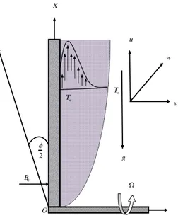
ORMULATION

Consider an unsteady MHD free convection flow past infinite vertical porous plate which is thermally stratified. Let us consider an unsteady free convective flow of an electrically conducting viscous fluid through a porous medium along a

semi-infinite vertical porous plate y0 in a rotating system under the influence of transversely applied magnetic field. The flow is assumed to be in the x-direction which is taken along the plate in the upward direction and y-axis is normal to it. Initially the fluid is at rest, after the whole system is allowed to rotate with a constant angular velocity

 _{about the y-axis. Since the systems rotate about}

the y-axis, so it is assumed as (0,,0). The

temperature of the plate raised from Tw _to T_,

where T be the temperature of the uniform flow. A uniform magnetic field B is taken to be acting along the y -axis which is assumed to be electrically non-conducting. There has been an

inclination angle 2

    

 _{with the vertical plate. The}

assumption is justified when the magnetic Reynolds number of the flow is taken to be small enough so that the induced magnetic field is negligible and is

of the form B (0,B0,0)_{and the magnetic lines of}

force are fixed relative to the fluid.

Fig. 1. Physical configuration and coordinate system.

Thus accordance with the above assumptions relevant to the problem and under the electromagnetic Boussinesq and non-Darcy approximation and neglecting hall current made by Chen and Lin (1995) Herman Schlichting (1969) and Chamkha (1996), in a rotating frame the basic boundary layer equations are given by;

The continuity equation

0

u v

x y

 _ _

  (1)

Momentum equations





2

1

2

u u u

u v g T T Cos

t x y





 

 _  _  _{ }  

_{  }   _{ }

 





2 2

2 2 0

2 2Ω

u B u

u c u w w

y k

  

 



     

 ₍₂₎

2

2 2

1 w w w w

u v w

t x y y k

 

 

 _  _  _  _

_{  }  _

 





2

2 2 ₂ B w0

c u w u 



     (3)

Energy equation

2

2

p

T T T k T

u v

t x y c y

 _  _  _ 

   

2  

X

Y 

0

B 

w

T

T

 g

O 

w





2 2 ₂

2 2

0

p p

u w B

u w

c y y c

   _{   }     _{ } _{ }            (4)

with the corresponding initial and boundary conditions are;

0, 0, 0, 0,

t u v  w  T T_

everywhere

(5)

0, 0, 0, 0, w at 0

t u v w TT Y 

0, 0, 0, at

u v  w  T T Y  

Where u v w, , are the velocity components in , ,

x y zdirections respectively,  is the kinematic viscosity,g is the acceleration due to gravity,  is

the density,k is thermal conductivity, B₀ be the uniform magnetic field,  be the porosity, C_pis the specific heat at constant pressure.

To obtain the governing equations and the boundary conditions in the dimensionless form, the following non-dimensional quantities are introduced as;

1/2 1/2 1/2

1/4 1/2

2

, , , ,

, and

r r r

r r

w

G uL G vL G wL x

U V w X

v v v L

G y G y T T

Y

L L T T

                

Substituting the above relations in equations (1)-(4) and after simplification, the following non-linear coupled partial differentials equations in terms of dimensionless variables are obtained as;

0

U V

X Y

 _ _

  (6)

2 2 2

2

U U U U

U V Cos

X Y  Y  

   _  _  _  _          









2 2_Γ 2 2 2 1 2

c

RW U W D M U

  

     (7)

. .

2 2 2

W W W W

U V RU

X Y  Y 



 _  _  _  _

   









2_Γ 2 2 2 1 2

c

U W D M W

  

    (8)

2 2 2 2 1 r U W U P V Ec

X Y Y Y Y

        _  _  _  _   _           _    _





2 2 2

T c

M E U W SU

   (9)

The corresponding initial and boundary conditions (5)-(6) becomes;

0,V 0,U 0,W 0, 0

      everywhere (10) 0,U 0,V 0,W 0, 1 S XT at Y 0

       

0, 0, 0, 0 at

U  V  W   Y  

where,

2

2_{( )}

r

p w

G Ec

C L T T







 (Eckert number)





3

2

w r

g T T L

G      (Grashofnumber), 2 r c k G D L 

(Darcy number), ΓCL(inertial parameter),

2 2Ω r L R G 

 (rotational parameter),

2 2 2 0 r L M G  

 (magnetic force parameter) and

, , ( ) x T w o T x S T T     

 (thermal stratification parameter).

3.

S

HEAR

S

TRESS AND

N

USSELT

N

UMBER

From the velocity field, the effects of various parameters on the local and average shear stress have been investigated. The following quantities represent the local and average shear stress at the plate.

Local shear stress, L ( )Y ₀

u y

   _

 and average

shear stress, _A ( u)_{Y 0}dx y

   _ 



which are

proportional to ( U)_{Y 0}

Y 



 and

100 0 0

( )Y

U Y  dX

 



respectively.

From the temperature field, the effects of various parameters on the local and average heat transfer coefficients have been investigated. The following equations represent the local and average heat transfer rate that is well known as Nusselt number.

Local Nusselt number,

0 uL Y T N y       _ _ 

  and

average Nusselt number, N_{u A} ( T)_{y 0}dx y

  _

 





which are proportional to ( T)_{Y 0}

Y 

 

 and

100

0 0

( T)_Y dX

Y 

 





respectively.

4.

N

UMERICAL

T

ECHNIQUE

To obtain the difference equations, the region of the flow is divided into a grid of lines parallel to

X

and

Y

axes where

X

-axes is taken along the plates and

Y

- axes is normal to the plates. It is considered that the plate of the heightXmax100

i.e,X varies from 0 to 100 and regard Y_max 25. There are m200 andn200grid spacing in the

X and

Y

directions respectively has been shown in the Fig.2

It has been assumed that  X, Y are constant mesh sizes along and directions respectively taken as follows;





0.5 0 100

X x

with the smaller time step,  0.001.

Fig. 2. Finite difference grid system.

Fig. 3. Grid independent test.

Here we have used the maximum mesh size (m=200 and n=200) for computing required result to get better accuracy. If we use less than the above mentioned mesh size then we will not get better result. If we consider higher mesh size then the program will not convergence due to shortage of memory of our computer. We have calculated the grid independent test for different mesh size;

. 300 , 300 and 295 , 295

; 290 , 290 ; 285 , 285 ; 280 , 280

; 275 , 275 ; 250 , 250 ; 225 , 225

; 200 , 200 ; 150 , 150 ; 100 , 100

  



     

     

     

n m n

m

n m n m n m

n m n m n m

n m n m n m

From these mesh size we have used m=200, n=200, because we get better accuracy for this mesh size

. If we used the mesh size more than , , then that will be time consuming and if we increase mesh size more than that like m=400, , then the program will not convergence. Here we have shown a figure of primary velocity for .7 below for the grid independent test

NowU,W denote the values ofU,W at the end of a time-step respectively. The explicit finite difference approximation gives;

Fig. 4. Primary velocity profiles for different values of dimensionless thermal stratification parameterS_T.

Fig. 5. Secondary velocity profiles for different values of dimensionless thermal stratification parameterST.

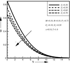
Fig. 6. Temperature profiles for different values of dimensionless thermal stratification

parameter ST

.

0 5 10

0 0.01 0.02 0.03

m=100; n=100 m=150; n=150 m=200; n=200 m=225; n=225 m=250; n=250 m=275; n=275 m=280; n=280 m=285; n=285 m=290; n=290 m=295; n=295 m=300; n=300

Y U

Pr=0.71

0 5 10

0 0.007 0.014 0.021 0.028

St=0.30

St=0.50

St=0.60

St=0.70

U

Y

M=0.10, R=0.10, Pr=0.71

Ec=0.10, Dc=0.20

 

0 2 4 6 8 10 12

-0.0001 -5E-05 0

St=0.30

St=0.50

St=0.60

S_t=0.70

W

Y

M=0.10, R=0.10, Pr=0.71

Ec=0.10, Dc=0.20

 

0 2 4 6 8 10 12 14 16

0 0.2 0.4 0.6

0.8 _S

t=0.30

St=0.50

S_t=0.60

St=0.70



Y

M=0.10, R=0.10, Pr=0.71

Ec=0.10, Dc=0.20

Fig. 7. Primary velocity profiles for different values of dimensionless Darcy numberDc

.

Fig. 8. Secondary velocity profiles for different values of dimensionless Darcy numberD_c

.

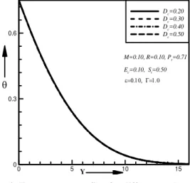
Fig. 9. Temperature profiles for different values of dimensionless Darcy numberD_c

.

, 1, , 1,

0

Δ Δ

i j i j i j i j

U U V V

X Y

 

 

  (11)

, , , 1, , 1 ,

, ,

Δ Δ Δ

i j i j i j i j i j i j

i j i j

U U U U U U

U V X Y         









2 2 2 2 1 2

, , ,

ΓUi j Wi j Dc M Ui j

  

    (12)

, , , 1, , 1 ,

, ,

Δ Δ Δ

i j i j i j i j i j i j

i j i j

W W W W W W

U V X Y         





, 1 , , 1 2 2 2 2

, , ,

2

2

Γ

(Δ ) i j i j i j

i j i j i j

W W W

RU U W

Y

      

   





2 1 2

,

c i j

D M W

 

  (13)

, , , 1, , 1 ,

, ,

Δ Δ Δ

i j i j i j i j i j i j

i j i j

U V X Y               





, 1 , , 1 2 2 2

, , ,

2

2 1

Ec (Δ )

i j i j i j

T i j i j j

r

i

S U M U W

Y P

     

   

, 1 , 2 , 1 , 2

[( ) ( ) ]

Δ Δ

i j i j i j i j

U U W W

Ec

Y Y

   

 

(14)

And the initial and boundary conditions with the finite difference scheme are;

0 0 0

, 0, , 0, , 0

i j i j i j

U  W   

,0 0, ,0 0, ,0 1

n n n

i i i T

U  W    S X

, 0, , 0, , 0

n n n

i L i L i L

U  W    where L 

Here the subscript iand jdesignates the grid points with xand ycoordinate and nrepresents a value of time  n  where n1, 2,3.... At the end of the time step , the new primary velocity

1 ,

n i j

U  , the new secondary velocity 1 ,

n i j

W  and the

new temperature distributions 1 ,

n i j

 

at all interior nodal points, may be calculated by successive applications of equations (11)-(14) respectively. Also the numerical values of the local shear stress and Nusselt number are evaluated by five-point approximation formula for their derivatives and the average shear stress and Nusselt number are

calculated by the use of the Simpson’s1

3integration formula.

Fig. 10. Primary velocity profiles for different values of dimensionless magnetic parameter M_.

0 5 10

0 0.007 0.014 0.021 0.028

Dc=0.20

Dc=0.30

Dc=0.40

D_c=0.50

Y U

M=0.10, R=0.10, Pr=0.71

Ec=0.10, St=0.50

 

0 5 10

-0.0001 -5E-05 0

Dc=0.20

Dc=0.30

Dc=0.40

Dc=0.50

Y W

M=0.10, R=0.10, Pr=0.71

Ec=0.10, St=0.50

 

0 5 10 15

0 0.3 0.6

Dc=0.20

Dc=0.30

Dc=0.40

D_c=0.50

Y



M=0.10, R=0.10, Pr=0.71

Ec=0.10, St=0.50

 

, 1 , , 1 2 2

, ,

2

2

(Δ ) 2

i j i j i j

i j i j

U U U

Cos RW

Y  



       

  _{ }

 

0 5 10

0 0.007 0.014 0.021 M=0.10 M=0.50 M=0.90 M=1.00 Y U

R=0.10, Pr=0.71, Ec=0.10

St=0.50, Dc=0.20

Fig. 11. Secondary velocity profiles for different values of dimensionless magnetic parameter M.

Fig. 12. Local primaryshear stress for different values of thermal stratification parmeter

 

ST

.

Fig. 13. Local secondaryshear stress for different values of thermal stratification parmeter

 

ST

.

5.

S

TABILITY AND

C

ONVERGENCE

A

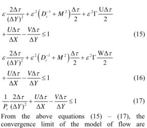
NALYSIS

Since an explicit procedure is being used, the analysis will remain incomplete unless the discussion of the stability and convergence of the finite difference Scheme. For the constant mesh size

the stability criteria of the scheme may be established as follows;





2 1 2 2

2

2Δ Δ UΔ

Γ

(ΔY) Dc M 2 2

  

 _  _{ }

Δ Δ

1

Δ Δ

U V

X Y

 

   (15)





2 1 2 2

2

2Δ Δ _ΓWΔ

(ΔY) Dc M 2 2

  

 _  _{ }

Δ Δ

1

Δ Δ

U V

X Y

 

   (16)

2

1 2Δ Δ Δ

1

(Δ ) Δ Δ

r

U V

P Y X Y

 _ _  _

(17)

From the above equations (15) – (17), the convergence limit of the model of flow are

0.51, 0.1, 1.90 andΓ 10

r c

P  D    .

Fig. 14. Average primaryshear stress for different values of thermal stratification

parmeter

 

S_T .

Fig. 15. Average secondary shear stress for different values of thermal stratification

parmeter

 

ST .

6.

R

ESULTS AND

D

ISCUSSIONS

The results have been presented for various values

0 5 10

-0.0001 -5E-05 0

M=0.10 M=0.50 M=0.90 M=1.00

Y

W R=0.10, Pr=0.71, Ec=0.10

St=0.50, Dc=0.20

 

0 25 50 75 100

0.03 0.06 0.09

St=0.30

St=0.40

St=0.50

St=0.60

X

X M=0.10, R=0.10, P_r=0.71

Ec=0.10, Dc=0.20

 

0 25 50 75 100

-0.0012 -0.0006 0

St=0.30

St=0.40

St=0.50

St=0.60

X

Y

M=0.10, R=0.10, Pr=0.71

Ec=0.10, Dc=0.20

 

20 40 60

4 6 8

St=0.30

St=0.40

St=0.50

St=0.60



X _{M=0.10, R=0.10, P}

r=0.71

Ec=0.10, Dc=0.20

 

20 40 60

-0.09 -0.06 -0.03

St=0.30

St=0.40

St=0.50

St=0.60

 Y

M=0.10, R=0.10, Pr=0.71

Ec=0.10, Dc=0.20

of thermal stratification parameter

 

ST , Darcy

number

 

Dc and magnetic parameter

 

M .Figs. 4

to 6 represented the primary, secondary velocity and the temperature distributions for different values of thermal stratification parameter

 

ST .

From these figure it has been observed that the primary velocity and temperature distribution decreases with the increases of the thermal stratification parameter

 

ST while the secondary

velocity increase with the increases of the values of thermal stratification parameter

 

ST . Figs. 7 to9

represented the primary, secondary velocity and the temperature distributions for different values of Darcy number

 

Dc . From these figure it has been

observed that the primary velocity increases with the increase of the Darcy number

 

Dc while the

secondary velocity decreases with the increase of the Darcy number

 

Dc .There exhibits minor

effects in the temperature distributions with the increasing values of Darcy number

 

Dc . Figs. 10

and 11 represented the primary and secondary velocity for different values of magnetic parameter

 

M . From these figure it has been observed that the primary velocity decreases with the increases magnetic parameter

 

M while the secondary velocity increases with the increases of magnetic parameter

 

M .

Fig. 16. Local primaryshear stress for different values of magnetic parameter

 

M .

Figs. 12 to 15 represented the local and average primary and secondary shear stress for different values of thermal stratification parameter

 

ST .

From these figures it has been observed that the local and average primary shear stress decreases with the increase of thermal stratification parameter

 

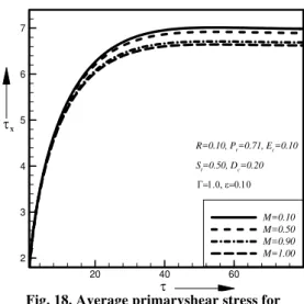
ST while the local and average secondary shear

stress increases with the increase of thermal stratification Figs.16to19represented the local and average primary and secondary shear stress for

different values of magnetic parameter

 

M . From these figures it has been observed that the local and average primary shear stress decreases with the increase of magnetic parameter

 

M while the local and average secondary shear stress increases with the increase of magnetic parameter

 

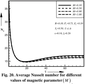
M . Fig. 20 represented the average Nusselt number for different values of magnetic parameter. From these figure it has been observed that the average nusselt number decreases with the increase of magnetic parameter

 

M .

Fig. 17. Local secondaryshear stress for different values of magnetic parameter

 

M .

Fig. 18. Average primaryshear stress for different values of magnetic parameter

 

M

.

9.

C

ONCLUSIONS

It has been observed that the primary velocity increases with the increase of Darcy number and while the reverse effect shows for thermal stratification parameter, Prandlt number and magnetic parameter. The secondary velocity increases with the increase of thermal stratification parameter, Prandlt number and magnetic parameter while the reverse effect shows for Darcy number. There has been cross flow shown for the primary

0 25 50 75 100

0.04 0.06

M=0.10 M=0.50 M=0.90 M=1.00

X

X

R=0.10, Pr=0.71, Ec=0.10

St=0.50, Dc=0.20

 

0 25 50 75 100

-0.0006 -0.0003

M=0.10 M=0.50 M=0.90 M=1.00

X

Y

R=0.10, P_r=0.71, E_c=0.10

St=0.50, Dc=0.20

 

20 40 60

2 3 4 5 6 7

M=0.10 M=0.50 M=0.90 M=1.00

 X

R=0.10, Pr=0.71, Ec=0.10

St=0.50, Dc=0.20

and secondary velocity for the porosity parameter. Temperature distributions decreases for thermal stratification parameter and Prandlt number and minor effects exhibits for Darcy number. Local and average primary shear stress increases for Darcy

number and porosity parameter while reverse effect shows for thermal stratification parameter and magnetic parameter. Local and secondary shear stress increases for thermal stratification parameter and magnetic parameter while reverse effect shows for Darcy number and porosity parameter.

Fig. 19. Average secondaryshear stress for different values of magnetic parameter

 

M

.

Fig. 20. Average Nusselt number for different values of magnetic parameter

 

M

.

REFERENCES

Agrawal, V. P., Agrawal, J. Kumar and N. K. Varsshney (2012). The effect of stratified viscous fluid on MHD free convection flow with heat and mass transfer past a vertical porous plate. Ultra Scientist 24, 139-146.

Angirasa, D. and J. Srinivasan, (1989). Natural convection flows due to the combine buoyancy of heat and mass diffusion in a thermally stratified medium. ASME Journal of Heat Transfer 111, 657-663.

Blottner, F. G., (1970), Finite-difference method of solution of a buoyancy layer equations. American Institute of Aeronautics and Astronautics 8, 193–205.

Chamkha, A. J. (1996). MHD free convection flow from a vertical plate embedded in a thermally stratified porous medium. Fluid/Particle Separation Journal 9, 195-206.

Chamkha, A. J., (1997), Hydromagnetic natural convection from an isothermal inclined surface adjacent to a thermally stratified porous medium. International Journal of Engineering Science, Vol. 35, pp. 975–986.

Chen, C. C. and R. Eichhorn, (1976). Natural convection from a vertical surface to a thermally stratified fluid. ASME Journal of Heat Transfer 98, 446-451.

Chen, C. K., C. I. Hung and W. C. Horng (1987). Transient natural convection on a vertical flat plate embedded in a high-porosity medium. American Society of Mechanical Engineers Journal of Energy Research technology 109, 112-118.

Chen, C. and C. Lin (1995). Natural convection from an isothermal vertical surface embedded in a thermally stratified high-porosity medium, International Journal of Engineering Science 31, 131-138.

Cowling,T. G. (1957. Magnetohydrodynamics, John Wiley & Sons, New York.

Fujii, T., M. Takuechi and I. Morioka (1974). Laminar boundary layer free convection in a temperature stratified environment. Proceedings of the 5th International Heat Transfer Conference, Tokyo, NC 2.2, 44–48.

Gebhart, B. and L. Pera (1971), “The natural of vertical natural convection flows resulting from the combined buoyancy effects of thermal and mass diffusion. International Journal of Heat and mass transfer 14, 2025-2050

Herrmann S. (1969). Boundary Layer Theory,John Wiley and Sons, New York.

Hossain, M. A., I. Pop and M. Ahamad (1996). MHD free convection flow from an isothermal plate. Journal of Theoretical and Applied Mechanics1, 94-207.

Saxena S. S. and G. K. Dubey (2011). Unsteady MHD heat and mass transfer free convection flow of polar fluids past a vertical moving porous plate in a porous medium with heat generation and thermal diffusion. Adva. Appl. Sci. Res. 2, 259-278.

Takhar, H. S., A .J. Chamka and G. Nath (2003). Effects of non-uniform wall temperature or mass transfer in finite sections of an inclined plate on the MHD natural convection flow in a temperature stratified high-porosity medium. International Journal of Thermal Sciences 42, 829–836.

20 40 60

-0.06 -0.03

M=0.10 M=0.50 M=0.90 M=1.00

 Y

R=0.10, Pr=0.71, Ec=0.10

St=0.50, Dc=0.20

 

20 40 60

15 20 25 30 35

M=0.10 M=0.50 M=0.90 M=1.00



Nu

R=0.10, Pr=0.71, Ec=0.10

St=0.50,

Venkatachala, B .J. and G. Nath (1981). Nonsimilar laminar natural convection in a thermally stratified fluid. International Journal of Heat Mass Transfer 24, 1348–1350.