DESEMPENHO DE UM ALGORITMO DE OTIMIZAÇÃO HIERÁRQUICO MULTIOBJETIVO APLICADO A UM MODELO DE SUPERFÍCIE
TERRESTRE E ECOSSISTEMAS
Dissertação apresentada à Universidade Federal de Viçosa, como parte das exigências do Programa de Pós-Graduação em Meteorologia Agrícola, para obtenção do título de Magister Scientiae.
VIÇOSA
“Come to the edge. We might fall. Come to the edge. It's too high! COME TO THE EDGE! And they came, And he pushed, And they flew“ Christopher Logue
“As botas apertadas são uma das maiores venturas da terra, porque, fazendo doer os pés, dão azo ao prazer de as descalçar”
AGRADECIMENTOS
À Universidade Federal de Viçosa (UFV) e ao Departamento de Engenharia Agrícola (DEA), pela oportunidade de realizar o curso de pós-graduação em Meteorologia Agrícola.
Ao Conselho Nacional de Desenvolvimento Científico e Tecnológico (CNPq), pela concessão da bolsa de estudos.
Ao meu amigo Victor Hugo Benezoli, por abrir as portas, me apoiar e auxiliar. Ao meu orientador, Prof. Marcos Heil Costa, pela oportunidade de desenvolver este projeto, pela paciência, pelo conhecimento compartilhado e pela grande amizade. À minha família, que é a minha base para todas as decisões de minha vida. E à minha segunda família, as D.I.V.A.S, que são amigas e companheiras e tornam a distância física dos meus consanguíneos um fato mais suave.
Ao Claudeci Varejão-Jr., que me esclareceu vários pontos deste trabalho e sempre foi muito atencioso.
Ao Fabrício Murta, por me salvar diversas vezes quando me perdi no código do programa, sempre de forma prestativa e divertida.
Aos meus amigos e companheiros do DEA, em especial aos do Grupo de Pesquisas em Interação Biosfera-Atmosfera: Patrícia, Gabrielle, Lívia, Francisca, Matheus, Letícia, Luciana.
BIOGRAFIA
CARLA CRISTINA DE SOUZA CAMARGOS, filha de Angela Maria de Souza Camargos (in memorian) e José Carlos Camargos, nasceu em 04 de novembro de 1985 na cidade de Carmo do Cajuru.
Em março de 2004, ingressou no curso de Matemática pela Universidade Federal de Viçosa (UFV).
Em setembro de 2008, estagiou no departamento de Tecnomatemática da Universidade de Bremen (Alemanha) por 3 meses.
SUMÁRIO
LISTA DE FIGURAS ... ix
LISTA DE TABELAS ... xi
LISTA DE SÍMBOLOS ... xii
RESUMO ... xiv
ABSTRACT ... xvii
1. INTRODUCTION ... 1
2. LITERATURE REVIEW... 5
2.1 Sensitivity analysis ... 5
2.2 Model evaluation ... 6
2.3 Multi-objective optimization ... 7
2.4 Genetic algorithms ... 7
2.5 Hierarchical optimization ... 8
3. METHODOLOGY ... 9
3.1 IBIS model ... 9
3.2 Site description and observed data...10
3.3 Data gap-filling and data filtering ...10
3.4 OPTIS ...12
3.5 IBIS’ sensitivity analysis ...12
3.6 Mono-objective calibration ...13
3.7 Multi-objective hierarchical calibration ...14
3.7.1 Comparison between simultaneous and hierarchical calibration ...15
3.7.2 Hierarchical calibration...16
4. RESULTS AND DISCUSSION ...18
4.1 IBIS’ sensitivity analysis ...18
4.3 Multi-objective calibration ...27
4.3.1 Comparison between simultaneous and hierarchical calibration ...27
4.3.2 Results for the hierarchical calibration ...30
4.4 Discussion on the performance index ...37
5. CONCLUSIONS ...40
LISTA DE FIGURAS
Figure 1: OPTIS structure.
Figure 2: PARo results after the mono-objective calibration: a) Dispersion plot and b) typical day using all 43 parameters and c) Dispersion plot and d) typical day using only sensitive parameters.
Figure 3: fAPAR results after the mono-objective calibration a) Dispersion plot and b) seasonal variation using all 43 parameters and c) Dispersion plot and d) seasonal variation using only sensitive parameters.
Figure 4: Rn results after the mono-objective calibration a) Dispersion plot and b) typical day using all 43 parameters and c) Dispersion plot and d) typical day using only sensitive parameters.
Figure 5: u* results after the mono-objective calibration a) Dispersion plot and b) typical day using all 43 parameters and c) Dispersion plot and d) typical day using only sensitive parameters.
Figure 6: H results after the mono-objective calibration a) Dispersion plot and b) typical day using all 43 parameters and c) Dispersion plot and d) typical day using only sensitive parameters.
Figure 7: LE results after the mono-objective calibration a) Dispersion plot and b) typical day using all 43 parameters and c) Dispersion plot and d) typical day using only sensitive parameters.
Figure 8: NEE results after the mono-objective calibration a) Dispersion plot and b) typical day using all 43 parameters and c) Dispersion plot and d) typical day using only sensitive parameters.
Figure 11: PARo results after the multi-objective calibration a) Dispersion plot and b) typical day.
Figure 12: fAPAR results after the multi-objective calibration a) Dispersion plot and b) seasonal variation.
Figure 13: Rn results after the multi-objective calibration a) Dispersion plot and b) typical day.
Figure 14: u* results after the multi-objective calibration a) Dispersion plot and b) typical day.
Figure 15: H results after the multi-objective calibration a) Dispersion plot and b) typical day.
Figure 16: LE results after the multi-objective calibration a) Dispersion plot and b) typical day.
Figure 17: NEE results after the multi-objective calibration a) Dispersion plot and b) typical day.
LISTA DE TABELAS
Table 1: Potential parameters for the calibration of IBIS.
Table 2: List of optimization experiments considering the group of variables related to radiative fluxes.
Table 3: List of optimization experiments considering the group of variables related to turbulent fluxes.
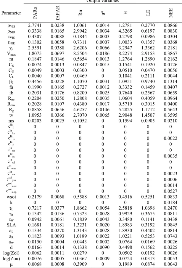
Table 4: Degree of sensitivity (µ* + σ) of all parameters for each output variables according to the Morris method.
Table 5: Parameters optimized in the calibration experiments related to radiative flux variables. Each pair of bracket represents one hierarchical level. Some parameters are not shown in the table because they are not used in any calibration below.
Table 6: MAE results for the mono-objective calibrations. fmono,overfit is the simulation using all 43 available parameters and fmono,SA is the simulation using only the parameters selected according to the sensitivity analysis validation
Table 7: Calibration results using only radiative flux output variables. The bracket is used to identify the hierarchical level, h is the number of hierarchical levels and n is the output quantity.
Table 8: Calibration results using only turbulent flux output variables. The bracket is used to identify the hierarchical level, h is the number of hierarchical levels and n is the output quantity.
LISTA DE SÍMBOLOS
aL Carbon allocation fraction to leaves (dimensionless)
aR Carbon allocation fraction to fine roots (dimensionless)
aW Carbon allocation fraction to wood (dimensionless)
β2 Parameter of fine roots distribution (Jackson rooting profile) (dimensionless)
CL Heat capacity of lower canopy leaves and stems ( J kg−1m−2)
clitll Carbon in leaf litter pool (lignin) (kg C m-2)
clitlm Carbon in leaf litter pool (metabolic) (kg C m-2)
clitls Carbon in leaf litter pool (structural) (kg C m-2)
clitrl Carbon in fine root litter pool (lignin) (kg C m-2)
clitrm Carbon in fine root litter pool (metabolic) (kg C m-2)
clitrs Carbon in fine root litter pool (structural) (kg C m-2)
clitwl Carbon in woody litter pool (lignin) (kg C m-2)
clitwm Carbon in woody litter pool (metabolic) (kg C m-2)
clitws Carbon in woody litter pool (structural) (kg C m-2)
CS Heat capacity of stems on upper canopy ( J kg−1m−2)
csoipas Carbon in soil (passive humus) (kg C m-2)
csoislon Carbon in soil (slow unprotected humus) (kg C m-2)
csoislop Carbon in soil (slow protected humus) (kg C m-2)
CU Heat capacity of upper leaves ( J kg−1m−2)
EA Evolutionary algorithm
fa Temperature function for aboveground biomass (stems) (dimensionless) fAPAR Fraction of absorbed photosynthetically active radiation
fb Temperature function for belowground biomass (roots) (dimensionless) GA Genetic algorithm
H Sensible heat flux
IBIS Integrated biosphere simulator
k Multiplication factor of decay constant for carbon pools (dimensionless) LE Latent heat flux
log(Zol) Logarithm of roughness length of lower canopy (dimensionless) log(Zou) Logarithm of roughness length of upper canopy (dimensionless) LSEM Land surface and ecosystem models
m Coefficient for stomatal conductance ( dimensionless) Average diffuse optical depth (dimensionless)
μ Mean effect of the model output parameters μ * Absolute value of μ
MAE Mean absolute error MBE Mean bias error
ms Factor of the soil moisture stress (dimensionless) MSE Mean square error
n The number of optimized objective functions NEE Net ecosystem exchange
xiv OAT One-step-at-a-time method
Rg Growth respiration coefficient (fraction) (dimensionless)
Rmr Maintenance respiration coefficient for root (s−1)
Rmw Maintenance respiration coefficient for wood (s−1)
RMSE Root mean square error Rn Net radiation
PARo Outgoing photosynthetically active radiation
ρNIR Leaf reflectance on upper canopy (NIR) (dimensionless) ρVIS Leaf reflectance on upper canopy (visible) (dimensionless)
AS Sensitivity analysis
SLA Specific leaf area (m2kg−1)
tv Vmax thermal stress (dimensionless)
L Foliage biomass turnover time constant (years)
NIR Leaf transmittance on upper canopy (NIR) (dimensionless) R Fine root biomass turnover time constant (years)
VIS Leaf transmittance on upper canopy (visible) (dimensionless) W Wood biomass turnover time constant (years)
u* Friction velocity (m s-1)
Vmax Maximum capacity of enzyme Rubisco at 15 °C on upper canopy (mol[CO2]
m−2s−1)
χu Leaf orientation factor on upper canopy (-1 vertical 0 random 1 horizontal)
RESUMO
CAMARGOS, Carla Cristina de Souza, M. Sc., Universidade Federal de Viçosa, março de 2013. Desempenho de um algoritmo de otimização hierárquico multiobjetivo aplicado a um modelo de superfície terrestre e ecossistemas. Orientador: Marcos Heil Costa.
ABSTRACT
CAMARGOS, Carla Cristina de Souza, M. Sc., Universidade Federal de Viçosa, March, 2013. Performance of a hierarchical multi-objective optimization
algorithm applied to a land surface and ecosystem model. Adviser: Marcos Heil
Costa.
The performance of LSEMs (Land surface and ecosystem models) depends on the
parameters of the equations representing the simulated process. However, the
measurement of some parameters can be impractical or even impossible; therefore,
they need to be estimated, or preferably optimized specifically for each ecosystem.
When the parameters are calibrated to a single variable (mono-objective problem)
they may not represent the reality, because the complexity of the model and its
dependence on several variables (multi-objective problem). Thus, simultaneous
multi-objective optimizations are indispensable. However, the optimization
performance decreases as the number of variables to be optimized simultaneously
increases. Furthermore, the study of simultaneous optimization using more than three
objectives is a new area and not yet sufficiently studied. For simultaneous
optimization of a large number of variables, there is a method that uses concepts of
hierarchical systems theory in which the optimization occurs from the fastest
(radiative fluxes) to the slowest process (carbon allocation). This study evaluates the
performance of the hierarchical optimization using the index D (the average of the
ratios between the individual outputs of multi-objective optimization and
mono-objective). Understanding how the performance index D varies with respect to the
number of objective functions optimized and to the number of hierarchical levels is
important for the development of this research area. Two steps are necessary to
achieve the study goals. First, a sensitivity analysis was performed to determine the
output variables sensitivity to the model parameters. After, simulations were made
using all possible combinations among the seven micrometeorological variables
available (PARo, fAPAR, Rn, u *, H, LE, NEE) taking into account the hierarchy of
processes. The results indicate that for up to three objective functions, hierarchical
objective optimization generates better results than the simultaneous
multi-objective optimization (one hierarchical level), provided that the parameters
Another important result shows that for the same number of outputs optimized, the
greater the number of hierarchical levels the better the performance of the optimized
model. However, the model performance falls quickly as the number of objective
functions increases, evidencing that the power of hierarchy calibration that use a high
number of objective functions is highly dependent on the removal of some
1. INTRODUCTION
Land surface and ecosystem models (LSEM) mechanistically describe ecosystem function in terms of biogeophysical processes (such as fluxes of sensible and latent heat, momentum and radiation), biogeochemical processes (terrestrial carbon cycle and CO2 fluxes) and ecological processes (phenology and competition among plant
functional types) at the biosphere-atmosphere interface. Land surface processes influence the climate system through their control of energy, water and carbon balances. Thus integrated LSEMs are important tools not only for biosphere-atmosphere interactions at long-term scales such as paleoclimates and future climates, but also for short-term applications that depend on land surface fluxes, like climate prediction and weather forecast.
Parameter calibration may be carried out using an optimization process that minimizes differences between predicted and observed data. Hence the increase in the number of calibrated parameters usually leads to a more reliable model. In addition to improving its performance, the calibration also allows for a detailed study of each of its components, so that the models can be improved according to necessity and resources [Pitman, 2003].
The performance of models with multiple outputs such as LSEMs could be optimized through the use of all available observations, including data collected by multiple sensors in intensive field sites and regional observations by remote sensors (radar, aircraft, satellites, etc). However, this improvement can increase the complexity of the optimization problem.
Each output variable simulated by the model (that has a corresponding observation) represents one objective of the optimization problem. There are two kinds of optimization: mono-objective and multi-objective. A mono-objective optimization has a unique solution to the problem, whereas in multi-objective problems, conflicting objectives are common, i.e., the optimized set of parameters for one objective function is not suitable for another. Thus a multi-objective problem may have a set of solutions instead of a unique solution to the problem. Hence there is a performance drop in simultaneous optimization methods with the increase of optimized objective functions in the same simulation [Deb et al., 2002; Veldhuizen and Lamont, 2000; Vrugt et al., 2003].
The simultaneous optimization of two or three objectives has been widely investigated [Gupta and Sorooshian, 1998; Deb et al., 2002; Coello, 2006] resulting in a variety of very efficient algorithms. The simultaneous optimization of more than three objectives, however, is a relatively young field and has not been thoroughly studied yet [Praditwong and Yao, 2007; Schutze et al., 2011].
slowest processes (carbon allocation). The concept is that a large number of objective functions can be optimized as long as (i) they are organized in hierarchical levels, which must contain no more than three objective functions of the same group to be simultaneously optimized; (ii) each model parameter is optimized only once (in one hierarchical level) during the optimization process. When the processes (objective functions) are separated in hierarchical levels, parameters that describe the processes should be distributed and optimized in only one hierarchical level. The selection of the parameters each process is most sensitive to is done through a sensitivity analysis. The hierarchical optimization technique was implemented in an algorithm (OPTIS), which was applied to the LSEM IBIS – Integrated Biosphere Simulator [Foley et al., 1996].
Assuming the mono-objective calibration is the best possible calibration for each individual output, the performance of the model after the multi-objective calibration can be compared to the performance of the mono-objective calibration of each independent variable by using a relative performance index (D) [Varejão-Jr. et al., 2012]. The index D is defined as the average of the individual ratios between the objective function output of the mono-objective calibration and the objective function output of the multi-objective calibration. The multi-objective hierarchical calibration efficiency is proportional to the value of the index D.
The way the performance of the optimization algorithm varies according to the number of optimized objective functions (n) is crucial to the optimization of LSEMs using intensive sites data. If the index D drops rapidly with number of objective functions then the optimization attempt may be useless, the LSEM calibration using all data collected at intensive sites is impossible and only the model validation is possible.
for determining the feasibility of the multi-objective optimization of LSEMs, in order to aid the design of model-improvement oriented intensive experimental sites and define future steps in land-surface/ecosystem modeling.
2. LITERATURE REVIEW
2.1 Sensitivity analysis
Sensitivity Analysis (SA) is an essential tool in modeling that helps to understand the importance of each parameter on the model output. An optimization problem can be very complex when it involves many parameters and multiple objective functions. Through SA, it is possible to understand how the variability in the model output may be attributed to the variability in the input [Rosolem et al., 2012]; and thus eliminate non-influential parameters in the optimization of some outputs, reducing the dimensions of the parameters space (screening method). Therefore, the search process becomes easier and the optimization results are improved.
the parameters in order of importance. However, such method does not quantify exactly the relative importance of each one.
Morris (1991) proposed the use of two different measures: one (µ) to estimate the mean effect of the model output parameters and another ( ) to estimate second and higher order effects (nonlinear effects and interactions). In order to avoid erroneous interpretations in non-monotonic models, Saltelli et al. (2005) proposed the use of the absolute value of the first measure proposed by Morris (|µ| = µ*).
The sensitivity results are never unique, because the SA algorithm uses a random value to begin the test. Furthermore, in nonlinear models, OAT could fail to account for the interactions among different input factors [Czitrom, 1999]. Thus multiple analyses are necessary to confirm the results, as described in Section 3.5.
2.2 Model evaluation
The model evaluation makes use of an objective function to yield numerical values which quantify how the predicted values fit the observed data. The choice of the adjustment metrics between prediction and observation for model calibration is even more important than the selection of the optimization method itself [Trudinger et al., 2007]. Several studies discuss the choice of adjustment metrics to evaluate accuracy and effectiveness of models [Fox, 1980; Willmott, 1981, 1982; Willmott et al., 1985; Legates and McCabe Jr., 1999; Willmott and Matsuura, 2005].
2.3 Multi-objective optimization
The multi-objective optimization deals with solving problems that have many objective functions. This technique finds a set of parameters which minimize or maximize simultaneously all the objective functions, generally satisfying some constraints. In multi-objective optimization problems, conflicting objectives require a set of optimal solutions (largely known as the Pareto set), instead of a single optimal solution, which is typically the case in mono-objective optimization problems [Veldhuizen and Lamont, 2000; Deb et al., 2002; Vrugt et al., 2003; Fu et al., 2005]. When an optimal solution cannot be replaced by one which improves an objective without worsening another, it is called a nondominated solution or Pareto-optimal solution. The plot of the objective functions whose nondominated solutions are in the Pareto set is called the Pareto frontier [Coello, 2006]. One of these Pareto-optimal solutions cannot be considered better than other without additional information, demanding the definition of as many Pareto-optimal solutions as possible [Deb et al., 2002].
2.4 Genetic algorithms
2.5 Hierarchical optimization
3. METHODOLOGY
3.1 IBIS model
The IBIS (Integrated Biosphere Simulator) was designed to connect land and hydrologic processes, land biogeochemical cycles and vegetation dynamics into a single modeling framework [Foley et al., 1996; Kucharik et al., 2000]. The model represents a wide range of processes, including land surface physics (solar and infrared radiative transfer through the canopy, turbulent processes, water interception and heat and mass transfer by canopy), canopy physiology, plant phenology, vegetation dynamics and competition, and carbon and nutrient cycling. All processes are hierarchically organized and operate on different time scales, from minutes (radiative fluxes) to years (carbon allocation). The model is forced by hourly inputs of air temperature and specific humidity, precipitation, wind speed, short- and long-wave incoming radiative fluxes.
photosynthetically active radiation (fAPAR), net radiation (Rn), friction velocity (u*), sensible heat flux (H), latent heat flux (LE) and net ecosystem exchange (NEE). IBIS has 43 potential parameters for calibration that are described in Table 1.
3.2 Site description and observed data
This study used data from an Amazon micrometeorological site: Tapajós National Forest (K67), an intensive field site located near km 67 of the Santarém-Cuiabá highway (02° 51’ 25’’S, 54° 58′ 15’’W), south of Santarém, Pará, Brazil. The typical land cover is evergreen broadleaf forest, formed mainly by evergreen and some semideciduous species. The forest spans 5 km to the east, 8 km to the south and 40 km to the north, before bordering pasture [Saleska et al., 2003]. Canopy height is 40 m on average, with emerging trees reaching up to 55 m [Costa et al., 2010].
This is an intensive data collection site, including measurements of meteorological variables (air temperature and specific humidity, precipitation, wind speed, short- and long-wave incoming radiative fluxes) and fluxes of mass, energy and momentum (PARo, fAPAR, Rn, u*, NEE, H, LE) [Saleska et al., 2003; Costa et al., 2010]. Other ecological measurements like leaf area index, net primary production and biomass were also taken at this site, but were not included in this study.
3.3 Data gap-filling and data filtering
Observed data used as model input usually present gaps. These data gaps were filled using interpolation, according to Senna et al. [2009]. This method uses three different equations: the first one is used when the gap duration is less than or equal to 3 hours, the second equation is used when the gap duration is greater than 3 hours or less than 24 hours and the third is used when the gap duration is greater than or equal to 24 hours.
Table 1: Potential parameters for the calibration of IBIS
Parameter name
Computational
notation Description
ρVIS rhoveg_vis Leaf reflectance on upper canopy (visible) (dimensionless)
ρNIR rhoveg_NIR Leaf reflectance on upper canopy (NIR) (dimensionless) VIS tauveg_vis Leaf transmittance on upper canopy (visible) (dimensionless)
NIR tauveg_NIR Leaf transmittance on upper canopy (NIR) (dimensionless)
χu chifuz
Leaf orientation factor on upper canopy (-1 vertical, 0 random, 1 horizontal)
Vmax vmax_pft
Maximum capacity of enzyme Rubisco at 15 °C on upper canopy (mol[CO2]m−2s−1)
m coefmub Coefficient for stomatal conductance (dimensionless)
CS chs Heat capacity of stems on upper canopy (J kg−1m−2)
CU chu Heat capacity of upper leaves (J kg−1m−2)
CL chl Heat capacity of lower canopy leaves and stems (J kg−1m−2)
β2 beta2
Parameter of fine roots distribution (Jackson rooting profile) (dimensionless)
fa funca_coef Temperature function for aboveground biomass (stems) (dimensionless)
fb funcb_coef Temperature function for belowground biomass (roots) (dimensionless)
Rmr rroot_coef Maintenance respiration coefficient for root (s−1)
Rmw rwood_coef Maintenance respiration coefficient for wood (s−1)
Rg rgrowth_coef Growth respiration coefficient (fraction) (dimensionless)
tv tempvm_coef Vmax thermal stress (dimensionless)
ms stressf_coef Factor of the soil moisture stress (dimensionless)
clitll clitll_coef Initial value of carbon in leaf litter pool (lignin) (kg C m-2)
clitlm clitlm_coef Initial value of carbon in leaf litter pool (metabolic) (kg C m-2)
clitls clitls_coef Initial value of carbon in leaf litter pool (structural) (kg C m-2)
clitrl clitrl_coef Initial value of carbon in fine root litter pool (lignin) (kg C m-2)
clitrm clitrm_coef Initial value of carbon in fine root litter pool (metabolic) (kg C m-2)
clitrs clitrs_coef Initial value of carbon in fine root litter pool (structural) (kg C m-2)
clitwl clitwl_coef Initial value of carbon in woody litter pool (lignin) (kg C m-2)
clitwm clitwm_coef Initial value of carbon in woody litter pool (metabolic) (kg C m-2)
clitws clitws_coef Initial value of carbon in woody litter pool (structural) (kg C m-2)
csoipas csoipas_coef Initial value of carbon in soil (passive humus) (kg C m-2)
csoislon csoislon_coef Initial value of carbon in soil (slow unprotected humus) (kg C m-2)
csoislop csoislop_coef Initial value of carbon in soil (slow protected humus) (kg C m-2)
wsoi wsoi_coef Initial soil moisture (m3m-3)
k kfactor Multiplication factor of decay constant for carbon pools (dimensionless)
L tauleaf Foliage biomass turnover time constant (years)
R tauroot Fine root biomass turnover time constant (years)
W tauwood0 Wood biomass turnover time constant (years)
SLA specla Specific leaf area (m2kg−1)
aL aleaf Carbon allocation fraction to leaves (dimensionless)
aR aroot Carbon allocation fraction to fine roots (dimensionless)
aW awood Carbon allocation fraction to wood (dimensionless)
d dispu_coef Zero-plane displacement height for upper canopy (m)
log(Zol) alogl_coef Natural logarithm of roughness length of lower canopy (dimensionless) log(Zou) alogu_coef Natural logarithm of roughness length of upper canopy (dimensionless)
second was the NEE filtering by a friction velocity threshold. Data was also eliminated from the analysis if the condition 0.6 < + < 1.4 was not satisfied for daily averages.
3.4 OPTIS
OPTIS, developed by Varejão-Jr. et al. (2012), is a hierarchical optimization algorithm based on the multi-objective genetic algorithm NSGA-II (Nondominated Sorted Genetic Algorithm II) [Deb et al., 2002]. This algorithm has limitations when dealing with a large number of objective functions at once, which accounts for loss of optimization efficiency [Luan et al., 1996]. Therefore, the maximum number of simultaneous objective functions considered in this study was three. In the multi-objective optimization, we can define the best solution for the optimization problem using different metrics [Fonseca et al., 1996; Deb et al., 2002]. This study considered as the best solution, the point with the smallest Euclidean distance from the origin in the Pareto frontier [Varejão-Jr. et al., 2012].
OPTIS was originally implemented to provide an automatic and multi-objective hierarchical calibration of the LSEM IBIS. The interaction between IBIS and OPTIS is minimal (Figure 1). The optimization algorithm changes the parameters of the model and reads its output data. In this way, IBIS is executed externally to the optimization algorithm and OPTIS is practically independent from the IBIS version or even from the model to be calibrated itself [Varejão-Jr. et al., 2012].
3.5 IBIS’ sensitivity analysis
The SA is able to detect which model parameters mostly influence the model results [Hamby, 1994] and how the variation in the output of a model can be apportioned in qualitative or quantitative terms [Saltelli et al., 2000; 2008]. In addition to the identification of each influential factor, the SA also tries to qualify their relative importance.
quantify the most sensitive parameters, the average of the sum of the measures µ* [Saltelli et al., 2005] and [Morris, 1991] were used.
Figure 1: OPTIS structure [Varejão et al., 2012].
3.6 Mono-objective calibration
3.7 Multi-objective hierarchical calibration
In a multi-objective hierarchical calibration each parameter can be associated to a single hierarchical level. Thus different results are expected for different arrangements of the same variables, since when the model is optimized at a certain hierarchical level, the parameters of the previous level have already been determined and remain fixed.
The best result (smallest MAE) between the two mono-objective runs (overfit and using SA) is the reference to analyze and understand the other calibrations, according to Equation 1. The comparison between mono-objective and hierarchical calibration provides a relative performance index (D) of the calibration method. The multi-objective calibration efficiency is proportional to the index D value.
The relative performance index D is defined as the average of the individual ratios between the objective function of the best mono-objective overfit calibration output (fmono) and the objective function of the multi-objective calibration output (fmulti). Mathematically,
1
1 n mono
i multi
i i
f D
n f (1)
where n is the number of objective functions and the D value should be between 0 and 1.
In order to organize the variables in hierarchical levels, the output variables were separated into two groups: the first related to radiative fluxes (PARo, fAPAR, Rn) and the second related to turbulent fluxes (u*, H, LE, NEE). Each group may be arranged in one or more hierarchical levels. Even though the order of the output variables within a group may be changed, the order in which the objective functions are optimized must be respected by the groups, because a necessary condition of the hierarchical approach is that the optimization moves from the fastest to the slowest process.
when such comparison was possible (n ≤ 3). Then the hierarchical calibration optimizing all model outputs was performed as described below.
To facilitate the interpretation of the results, the multi-objective hierarchical calibration was divided in three parts. Initially, only output variables related to radiative fluxes were optimized, as described in section 3.7.1. Two or three variables were hierarchically optimized, considering one or two hierarchical levels (Table 2). Afterwards, only output variables related to turbulent fluxes were optimized, as shown in section 3.7.1. A number from two to four variables were hierarchically optimized, considering one or two hierarchical levels as well (Table 3).
Finally, the output variables of any of the previous groups were optimized (section 3.7.2). A number from two to seven variables were hierarchically optimized, with the number of hierarchical levels varying from two to four.
3.7.1 Comparison between simultaneous and hierarchical calibration
Two methods of calibration were compared for the group of variables related to radiative fluxes (PARo, fAPAR and Rn) as well as for the group of variables related to turbulent fluxes (u*, H, LE, NEE). Hereinafter, curly brackets {} were used to identify output variables that were simultaneously optimized. Hence the simultaneous calibration is denoted by all variables in the same bracket (e.g., {PARo-fAPAR-Rn}), whereas the hierarchical calibration is denoted by a sequence of brackets, e.g. {PARo-fAPAR}{Rn}, in which the variables were optimized following the brackets sequence.
There are ten different simulation combinations that can be separated in four simulations using one hierarchical level (simultaneous calibration) and six simulations using two hierarchical levels (Table 2).
It is also important to highlight in Table 2 that PARo and fAPAR are present either individually or in the same hierarchical level, but not in two different hierarchical levels. This is explained by the fact the parameter χu is as important to PARo as to
fAPAR, so they must either be optimized simultaneously or individually, but not sequentially.
To optimize the turbulent fluxes variables, there are twenty-four different simulation combinations that can be separated in ten simulations using one hierarchical level (simultaneous calibration) and fourteen simulations using two hierarchical levels (Table 3). As explained for radiative flux variables, because the order of hierarchical levels may affect the results, all combinations were tested.
Table 2: List of optimization experiments considering the group of variables related to radiative fluxes.
Simultaneous Hierarchical {PARo-fAPAR}
{PARo-Rn} {PARo}{Rn}
{Rn}{PARo}
{fAPAR-Rn} {fAPAR}{Rn}
{Rn}{fAPAR}
{PARo-fAPAR-Rn} {PARo-fAPAR}{Rn}
{Rn}{PARo-fAPAR}
The variables H, LE and NEE cannot be separated in different hierarchical levels because the most sensitive parameters for them are the same (β2,Vmax, Rg and others),
thus they must be optimized simultaneously in the same hierarchical level.
3.7.2 Hierarchical calibration
113 using five output variables, 45 using six output variables and 6 simulations using all seven output variables.
The combination of variables was carried out as described in section 3.7.1, emphasizing that variables from different groups (radiative and turbulent fluxes) cannot be calibrated simultaneously in the same hierarchical level because the main assumption of the hierarchical optimization is that it is performed from the fastest to the slowest processes.
Table 3: List of optimization experiments considering the group of variables related to turbulent fluxes.
Simultaneous Hierarchical {H-LE}
{H-NEE}
{LE-NEE}
{u*-H} {u*}{H}
{H}{u*}
{u*-LE} {u*}{LE}
{LE}{u*}
{u*-NEE} {u*}{NEE}
{NEE}{u*}
{H-LE-NEE}
{u*-H-LE} {u*}{H-LE}
{H-LE}{u*}
{u*-H-NEE} {u*}{H-NEE}
{H-NEE}{u*}
{u*-LE-NEE} {u*}{LE-NEE}
{LE-NEE}{u*}
{u*}{H-LE-NEE}
4. RESULTS AND DISCUSSION
4.1 IBIS’ sensitivity analysis
A rank determining the sensitivity of each variable to each parameter was built using the average of ten sensitivity measures (µ* + ) (Table 4). The greater the sum, the more sensitive is the model to that parameter. As shown in Table 4, PARo, fAPAR, Rn, H and LE are sensitive to 30 parameters, u* to 25 parameters and NEE to 37 parameters.
When the variables are separated into different hierarchical levels, it is possible to choose which parameters will be in each hierarchical level, considering that one parameter can be calibrated only once. Such decisions were made according to the degree of sensitivity shown in Table 4.
Table 4: Degree of sensitivity (µ* + ) of all parameters for each output variables according to the Morris method. Unit of the degree of sensitivity is the same of the output variable. Output variables Parameter P A R o fA P A R
Rn u* H LE NEE
ρVIS 2.7741 0.0238 1.0061 0.0014 1.2781 0.2770 0.0866
ρNIR 0.3338 0.0165 2.9942 0.0034 4.3265 0.6197 0.0830 VIS 0.4307 0.0088 0.1844 0.0003 0.2798 0.0986 0.0304 NIR 0.1302 0.0058 0.7311 0.0007 1.0033 0.1357 0.0368
χu 2.5591 0.0388 2.6206 0.0066 3.2947 1.3362 0.2181
Vmax 1.8075 0.0697 8.5504 0.0186 8.2274 2.9153 0.3867
m 0.1847 0.0146 0.5654 0.0013 1.2764 1.2890 0.2162 CS 0.0074 0.0013 0.0847 0.0015 0.1541 0.1920 0.0126
CU 0.0049 0.0003 0.0300 0 0.0510 0.0470 0.0056
CL 0.0040 0.0007 0.0469 0 0.1041 0.2111 0.0044
β2 0.4456 0.0228 1.1070 0.0031 1.0951 0.9740 0.1314
fa 0.1990 0.0165 0.2727 0.0012 0.3332 0.1459 0.0407 fb 0.2031 0.0176 0.8200 0.0025 0.7640 0.2567 0.0659 Rmr 0.2204 0.0250 1.2808 0.0035 1.0604 0.4059 0.0964
Rmw 0.2028 0.0107 0.4380 0.0017 0.5719 0.3015 0.0400
Rg 0.8858 0.0656 4.6257 0.0146 5.2825 1.1712 0.5643
tv 1.0953 0.0366 2.7070 0.0065 2.9048 1.4507 0.3595 ms 0.0203 0.0025 0.1052 0 0.1594 0.0905 0.0210
clitll 0 0 0 0 0 0 0
clitlm 0 0 0 0 0 0 0
clitls 0 0 0 0 0 0 0.0022
clitrl 0 0 0 0 0 0 0
clitrm 0 0 0 0 0 0 0
clitrs 0 0 0 0 0 0 0.0035
clitwl 0 0 0 0 0 0 0
clitwm 0 0 0 0 0 0 0
clitws 0 0 0 0 0 0 0.0023
csoipas 0 0 0 0 0 0 0.0006
csoislon 0 0 0 0 0 0 0.0014
csoislop 0 0 0 0 0 0 0.0527
wsoi 0.2179 0.0068 0.5588 0.0013 0.4516 0.5251 0.0833
k 0 0 0 0 0 0 0.0184
L 0.7217 0.0377 1.8662 0.0054 2.5818 1.0698 0.2470 R 0.1342 0.0136 0.7323 0.0028 0.9929 0.3675 0.0811 W 0.0942 0.0061 0.1839 0.0043 0.3480 0.1141 0.0438
SLA 0.1681 0.0181 1.3231 0.0020 1.8983 0.3192 0.0845 aL 0.1334 0.0270 1.3143 0.0028 1.8930 0.4402 0.0814
aR 0.1823 0.0093 1.0189 0.0022 1.0221 0.5253 0.0743
aW 0.0150 0.0004 0.0443 0.0002 0.0764 0.0169 0.0026
d 0.0166 0.0014 0.1338 0.0090 0.4498 0.1562 0.0225 log(Zol) 0.0062 0.0011 0.0279 0 0.0502 0.0192 0.0026 log(Zou) 0.0076 0.0005 0.0367 0.0009 0.0724 0.0313 0.0053
Table 5: Parameters optimized in the calibration experiments related to radiative flux variables. Each pair of bracket represents one hierarchical level. Some parameters are not shown in the table because they are not used in any calibration below.
Output Variables
One hierarchical level Two hierarchical levels
Parameter {PARo-fAPAR} {PARo-Rn} {fAPAR-Rn} {PARo-fAPAR-Rn} {PARo}{Rn} {Rn}{PARo} {fAPAR}{Rn} {Rn}{fAPAR} {PARo-fAPAR}{Rn} {Rn}{PARo-fAPAR}
ρVIS x x x x x x x x x x
ρNIR x x x x x x x x x x
VIS x x x x x x x x x x
NIR x x x x x x x x x x
χu x x x x x x x x x x
Vmax x x x x x x x x x x
m x x x x x x x x x x
CS x x x x x x x x x
CU x x x x x x x x x
CL x x x x x x x
β2 x x x x x x x x x x
fa x x x x x x x x x x
fb x x x x x x x x x x
Rmr x x x x x x x x x x
Rmw x x x x x x x x x x
Rg x x x x x x x x x x
tv x x x x x x x x x x
ms x x x x x x x x x x
wsoi x x x x x x x x x x
L x x x x x x x x x x
R x x x x x x x x x x
W x x x x x x x x x x
SLA x x x x x x x x x x
aL x x x x x x x x x x
aR x x x x x x x x x x
aW x x x x x x x x x x
d x x x x x x x x x x
log(Zol) x x x x x x
log(Zou) x x x x x x x x x
to get a satisfactory result of fAPAR. Furthermore, Rn does not present a good fit if simulated with many parameters calibrated to fAPAR. The same happens when Rn is in the first hierarchical level and is calibrated using only three parameters.
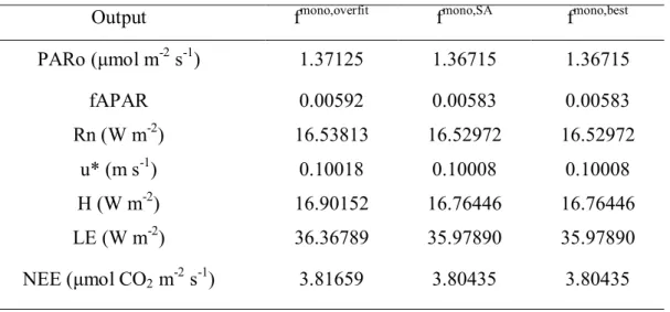
4.2 Mono-objective calibration
Mono-objective calibrations were performed in two different ways: calibrations using all 43 available parameters (overfit) and calibrations using only the sensitive parameters (Table 4). The MAE results for both mono-objective calibrations are shown in Table 6. For the seven optimized variables, the optimizations using only the SA parameters produced the smallest MAE in all cases.
Table 6: MAE results for the mono-objective calibrations. fmono,overfit is the simulation using all 43 available parameters and fmono,SA is the simulation using only the parameters selected according to the sensitivity analysis validation
Output fmono,overfit fmono,SA fmono,best
PARo (μmol m-2
s-1) 1.37125 1.36715 1.36715
fAPAR 0.00592 0.00583 0.00583
Rn (W m-2) 16.53813 16.52972 16.52972
u* (m s-1) 0.10018 0.10008 0.10008
H (W m-2) 16.90152 16.76446 16.76446
LE (W m-2) 36.36789 35.97890 35.97890
NEE (μmol CO2 m-2 s-1) 3.81659 3.80435 3.80435
In order to understand the MAE results, dispersion and typical day plots were produced for each mono-objective calibration. According to Figures 2-8, most outputs (except fAPAR and Rn) fit better to the data when only the sensitive parameters were used.
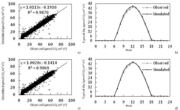
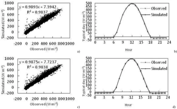
Figure 2 shows the nearly perfect fit of the hourly data of PARo. The model slightly overestimated PARo between 9 and 12 hours and underestimated PARo in the first hours of the night (Figure 2-b and d). The regression coefficients were a = 1.01 and b = -0.19 for the overfit calibration (Figure 2-a) and a = 1.00 and b = -0.14 for the SA calibration (Figure 2-c).
a) b)
c) d)
Figure 2: PARo results after the mono-objective calibration: a) Dispersion plot and b) typical day using all 43 parameters and c) Dispersion plot and d) typical day using only sensitive parameters.
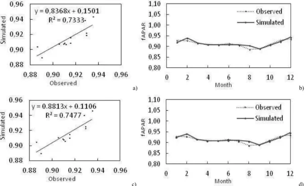
and b = 0.15 for the overfit calibration (Figure 3-a) and a = 0.88 and b = 0.11 for the SA calibration (Figure 3-c).
Figure 4 shows the nearly perfect fit of the hourly data of Rn. The difference between both mono-objective calibrations of Rn was small. The regression coefficients were a = 0.99 and b = 7.39 for overfit calibration (Figure 4-a) and a = 0.99 and b = 7.72 for the SA calibration (Figure 4-c).
a) b)
c) d)
Figure 3: fAPAR results after the mono-objective calibration a) Dispersion plot and b) seasonal variation using all 43 parameters and c) Dispersion plot and d) seasonal variation using only sensitive parameters.
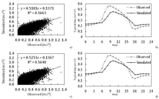
overfit calibration (Figure 5-a) and a = 0.53 and b = 0.14 for the SA calibration (Figure 5-c).
Figure 6 shows the mono-objective calibration of H. The bias between observed and simulated data was small and the overestimation of H was noticeable during the night (Figure 6-b and d). On the other hand, H simulations during daytime were satisfactory. The regression coefficients were a = 0.73 and b = 13.13 for the overfit calibration (Figure a) and a = 0.76 and b = 13.06 for the SA calibration (Figure 6-c). This was a fairly surprising result, considering that the model does not generate enough turbulence (Figure 5) and means that OPTIS has found a way to improve the IBIS simulation for H, by excessively heating up the canopy during daytime, through changes in the net radiation and leaves heat capacity (results not shown). This is a common behavior in mono-objective optimizations, indicating the need for multiple output optimizations.
a) b)
c) d)
Figure 7 shows the mono-objective calibration of LE. The model was not able to estimate the high values during the day, causing a bias of about 80 W m-2 in the daily peak (Figure 7-b and d). This is a direct consequence of the low turbulence generated by the model, although, contrary to H, in this case the optimizer apparently could not find alternative ways to increase LE values. The regression angular coefficients were a = 0.59 for the overfit calibration (Figure 7-a) and a = 0.60 for the SA calibration (Figure 7-c), just slightly higher than the angular coefficient for the u* optimization (a = 0.52).
Figure 8 shows the mono-objective calibration of NEE. The model overestimated NEE during the day and there was an advance of one hour in the minimum value (Figure 8-b and d). The regression coefficients were a = 0.76 and b = -1.02 for the overfit calibration (Figure 8-a) and a = 0.76 and b = -0.99 for the SA calibration (Figure 8-c).
a) b)
c) d)
a) b)
c) d)
Figure 6: H results after the mono-objective calibration a) Dispersion plot and b) typical day using all 43 parameters and c) Dispersion plot and d) typical day using only sensitive parameters.
a) b)
c) d)
a) b)
c) d)
Figure 8: NEE results after the mono-objective calibration a) Dispersion plot and b) typical day using all 43 parameters and c) Dispersion plot and d) typical day using only sensitive parameters.
4.3 Multi-objective calibration
4.3.1 Comparison between simultaneous and hierarchical calibration
{PARo-fAPAR}{Rn}, and only 0.8222 for the simultaneous configuration {PARo-fAPAR-Rn}.
Table 7: Calibration results using only radiative flux output variables. The bracket is used to identify the hierarchical level, h is the number of hierarchical levels and n is the output quantity.
, mono best multi f f
h n Optimization
configuration PARo fAPAR Rn Index D
1 2 {PARo-fAPAR} 0.9726 0.7447 - 0.8586
1 2 {PARo-Rn} 0.8582 - 0.9676 0.9129
2 2 {PARo}{Rn} 0.9699 - 0.9661 0.9680
2 2 {Rn}{PARo} 0.9707 - 0.9867 0.9787
1 2 {fAPAR-Rn} - 0.6796 0.8405 0.7600
2 2 {fAPAR}{Rn} - 0.8235 0.9103 0.8669
2 2 {Rn}{fAPAR} - 1.0294 0.7246 0.8770
1 3 {PARo-fAPAR-Rn} 0.8888 0.7527 0.8250 0.8222
2 3 {PARo-fAPAR}{Rn} 0.9334 0.6250 0.9746 0.8443
2 3 {Rn}{PARo-fAPAR} 0.9587 0.7955 0.9304 0.8948
configuration using u* in the second hierarchical level ({H-LE}{u*}, {H-LE}{u*}, {LE-NEE}{u*}).
Figure 9: Index D for radiative flux output variables as a function of the number of optimized outputs (n), separated by the type of optimization (simultaneous or hierarchical).
Figure 10: Index D for turbulent flux output variables as a function of the number of optimized outputs (n), separated by the type of optimization (simultaneous or
hierarchical). 0.72 0.76 0.80 0.84 0.88 0.92 0.96 1.00
0 1 2 3 4
In d e x D n
Simultaneous Hierarchical
0.80 0.84 0.88 0.92 0.96 1.00
0 1 2 3 4 5
In d e x D n
Table 8: Calibration results using only turbulent flux output variables. The bracket is used to identify the hierarchical level, h is the number of hierarchical levels and n is the output quantity.
, mono best
multi f
f
h n Optimization
configuration u* H LE NEE Index D
1 2 {H-LE} - 0.9451 0.9093 - 0.9272
1 2 {H-NEE} - 0.7243 - 1.0090 0.8666
1 2 {LE-NEE} - - 0.8757 0.9666 0.9211
1 2 {u*-H} 0.9806 0.9774 - - 0.9790
2 2 {u*}{H} 0.8510 0.9802 - - 0.9156
2 2 {H}{u*} 1.0000 0.9970 - - 0.9985
1 2 {u*-LE} 0.9517 - 0.9507 - 0.9512
2 2 {u*}{LE} 0.8623 - 0.9967 - 0.9295
2 2 {LE}{u*} 0.9459 - 0.9919 - 0.9689
1 2 {u*-NEE} 0.9011 - - 0.9765 0.9388
2 2 {u*}{NEE} 0.8510 - - 0.9991 0.9250
2 2 {NEE}{u*} 0.8178 - - 1.0465 0.9322
1 3 {H-LE-NEE} - 0.9075 0.8990 0.9757 0.9274
1 3 {u*-H-LE} 0.9726 0.8713 0.9436 - 0.9292
2 3 {u*}{H-LE} 0.8510 0.9464 0.9209 - 0.9061
2 3 {H-LE}{u*} 0.9808 0.9563 0.9101 - 0.9491
1 3 {u*-H-NEE} 0.8764 0.7180 - 0.9398 0.8447
2 3 {u*}{H-NEE} 0.8623 0.8707 - 0.9074 0.8801
2 3 {H-NEE}{u*} 0.9715 0.9158 - 0.9962 0.9612
1 3 {u*-LE-NEE} 0.8711 - 0.8170 0.9797 0.8892
2 3 {u*}{LE-NEE} 0.8510 - 0.9831 0.9555 0.9299
2 3 {LE-NEE}{u*} 0.9484 - 0.9467 0.9736 0.9563
2 4 {u*}{H-LE-NEE} 0.8510 0.8720 0.9407 0.9343 0.8995
2 4 {H-LE-NEE}{u*} 0.9759 0.8827 0.9153 0.9830 0.9392
4.3.2 Results for the hierarchical calibration
The analysis of the hierarchical calibration results indicates that it is possible to underline some combinations of variables that generate the best results and also to identify the position of each variable and the distribution of parameters among the hierarchical levels to provide for the best fit of observed data.
in the configuration {Rn}{fAPAR}, the ratio fmono/fmulti for fAPAR was greater than one, i.e., the mono-objective calibration was not the best possible calibration. There are two possible explanations: either the number of parameters used was more than necessary or the values used for the baseline parameters were not the most appropriate.
For turbulent flux variables, the best result was always obtained when u* was in the second hierarchical level and H or/and LE or/and NEE were in the first hierarchical level (Table 8). The same discussion presented for fAPAR can be applied to NEE in two cases: configurations {H-NEE} and {NEE}{u*}.
For radiative and turbulent fluxes, confirming the trend of the previous results, the best result considering the index D (Table 9) occurred for the order below:
1° hierarchical level: Rn
2° hierarchical level: PARo and fAPAR 3° hierarchical level: H, LE and NEE 4° hierarchical level: u*
Hierarchical calibration performs a global calibration of the model and optimizes, as well as possible, all variables simultaneously. As expected, the individual results for hierarchical calibration are worse than the results for the mono-objective calibration. In order to understand the hierarchical calibration results, the dispersion and typical day plots were produced for each individual variable of the best seven-objective calibration (Figures 11-17). These results can be compared to those obtained for the mono-objective calibration, presented in Figures 2 to 8.
Table 9: Calibration results using radiative and turbulent flux output variables. The bracket is used to identify the hierarchical level, h is the number of hierarchical levels and n is the output quantity.
, mono best
multi f
f
h n Output PARo fAPAR Rn u* H LE NEE Index D
3 7 {PARo-Rn-fAPAR}{ustar}{H-LE-NEE} 0.6706 0.5556 0.7468 0.8856 0.2626 0.7031 0.7298 0.6506
4 7 {PARo-fAPAR}{Rn}{ustar}{H-LE-NEE} 0.9476 0.6140 0.7192 0.8882 0.2720 0.7524 0.6555 0.6927
4 7 {Rn}{PARo-fAPAR}{ustar}{H-LE-NEE} 0.7944 0.6481 0.7246 0.8863 0.2733 0.7242 0.8479 0.6998
3 7 {PARo-Rn-fAPAR}{H-LE-NEE}{ustar} 0.6706 0.5556 0.7468 0.9136 0.2723 0.7228 0.7901 0.6674
4 7 {PARo-fAPAR}{Rn}{H-LE-NEE}{ustar} 0.9476 0.6140 0.7192 0.8920 0.2761 0.7174 0.8037 0.7100
a) b)
Figure 11: PARo results after the multi-objective calibration a) Dispersion plot and b) typical day.
Figure 12 shows fAPAR after the hierarchical calibration. Monthly data presented good fit, with overestimated results during the winter (Figure 12-b). The regression coefficients were a = 0.76 and b = 0.23 (Figure 12-a).
Figure 14 shows the multi-objective calibration of u*. As observed for the mono-objective calibration, the model overestimated u* during the day and underestimated u* during the night, with a delay of one hour in the maximum value (Figure 14-b). The regression coefficients were a = 0.44 and b = 0.16 (Figure 14-a).
a) b)
a) b)
Figure 13: Rn results after the multi-objective calibration a) Dispersion plot and b) typical day.
a) b)
Figure 14: u* results after the multi-objective calibration a) Dispersion plot and b) typical day.
a) b)
Figure 15: H results after the multi-objective calibration a) Dispersion plot and b) typical day.
a) b)
Figure 16: LE results after the multi-objective calibration a) Dispersion plot and b) typical day.
The results for H, LE and NEE were remarkably different from those obtained for the mono-objective optimization. All three variables must be optimized simultaneously, in the third hierarchical level, because the three output variables are sensitive to the same parameters. It was observed earlier that the simultaneous optimization usually decreases the algorithm’s performance, and this became very clear when comparing Figures 15-17 to Figures 6-8. Because of several constraints in this optimization (including H, LE and NEE in the same hierarchical level and energy conservation by the model), the optimizer chose parameters that reduced stomatal conductance and increased canopy temperature (results not shown).
in Table 8). Although the drop in the ratio fmono/fmulti is an expected characteristic of the hierarchical multi-objective optimization as the number of objectives increase, in no other optimized variable the performance presented such a significant drop. In addition to the constraints already discussed, an important characteristic of the observed and the simulated data was co-responsible for this result: whereas the model must conserve energy (Rn – G = LE + H), the observed energy flux data obtained from net radiometers and eddy covariance systems is rarely conservative, and Rn – G is usually greater than LE + H (See Twine et al. [2000] for a general discussion, or Costa et al. [2010] for a discussion specific for this site).
Given these errors in the data, the optimizer tends to make different choices in the mono or multi-objective optimizations. In the H mono-objective optimization, there is no constraint on Rn simulation, so the optimizer can freely modify it to provide the adequate net radiation for the correct simulation of H. In the multi-objective optimization, simulated Rn matches the observations, which eliminates the possibility of any energy adjustments, and more radiative energy must be portioned between the two turbulent fluxes (G is about 1% of Rn, so it was not considered in this discussion).
An attempt to compensate this problem in energy balance closure was made by using only Rn, LE and H values in days when LE + H was within 40% of Rn (see discussion in Costa et al. [2010]). However even after filtering, in most days, Rn was significantly different from LE + H. A better approach to correct this problem may be to correct LE and H according to the observed Bowen ratio, so that long-term LE + H matches long-term Rn, as proposed by Twine et al. [2000]. This would ensure energy conservation in the long-term observed data.
Figure 17 shows the multi-objective calibration of NEE. The model bias at midday was about 7 μmol CO2 m-2 s-1 and there was an advance of one hour in the minimum
a) b)
Figure 17: NEE results after the multi-objective calibration a) Dispersion plot and b) typical day.
4.4 Discussion on the performance index
Figure 18 shows all results of the performance index D versus the number of optimized outputs, separated by the number of hierarchical levels, from 1 to 4. Four conclusions can be drawn from this figure.
First, it is generally true that, for the same number of optimized outputs, the higher the number of hierarchical levels used, the better the performance of the optimized model (higher D). This is in agreement with the detailed analysis provided in Section 4.3.1.
Figure 18: Index D for radiative and turbulent flux output variables versus the number of optimized outputs (n), separated by the type of optimization (simultaneous or hierarchical).
Third, results indicate that D drops at faster rates if n increases. This seems to be a consequence of the constraints introduced by the need to simultaneously optimize specific variables, notably fAPAR and PARo, and NEE, H and LE, which are sensitive to the same parameters. Further research on the criteria to select the parameters to be optimized at each hierarchical level may remove some of these constraints, and may help improve the model results for a large value of n.
0.52 0.54 0.56 0.58 0.60 0.62 0.64 0.66 0.68 0.70 0.72 0.74 0.76 0.78 0.80 0.82 0.84 0.86 0.88 0.90 0.92 0.94 0.96 0.98 1.00
0 1 2 3 4 5 6 7 8
Ind
e
x
D
n
Simultaneous 2 hierarchical levels
5. CONCLUSIONS
An evaluation of the efficiency of an algorithm of hierarchical calibration, which is based in the temporal organization of natural ecosystems and of the IBIS land surface/ecosystem model was carried out. The automatic system of calibration (OPTIS) is based in the multi-objective genetic algorithm NSGA-II and enables the calibration of many (more than 3) output variables. The application of OPTIS allows for the general calibration of the model, adjusting the variables simulated by IBIS in a more reliable way. This study used the sensitivity analysis developed by Morris to select the most important parameters for calibration. Sensitivity analysis is the most important step for a well fit model, because the results are highly dependent on the distribution of the parameters in the hierarchical levels. Furthermore, in a mono-objective calibration, the variable fits better to the data if it is calibrated using only the sensitive parameters and not all the available ones.
(radiative flux variables PARo and fAPAR, and turbulent flux variables H, LE and NEE) and the difficulty in selecting parameters to be optimized in each hierarchical level, resulted in a faster drop of D as n increased. The decrease in the slope of the D x n curve is desirable, since the use of more measurements at different time scales is the only way to comprehensively improve models.
Model’s performance depends on the optimization configuration. As a first rule, this study identified that the configuration responsible for the best model fit occurs if Rn is calibrated before PARo and fAPAR, and u* is calibrated after H, LE and NEE. However, the model’s performance after optimization is extremely sensitive to variations in the allocation of parameters to each hierarchical level. The choice of these parameters is in principle governed by the results of the sensitivity analysis. Nevertheless, the qualitative nature of the Morris method, its inability to evaluate the interactions among parameters, as well as its random nature, limited the role of the SA in the parameter decision process, and considerable modeler intuition was used to allocate the parameters to each hierarchical level. Although it is likely that the index D for model’s performance will always decrease with the increase of n, it may be possible to keep the decrease rate in the range of 1% of D per objective added to the problem (per unitary increase in n). This was the rate obtained in this study before constraints started to decrease the optimizer’s performance, and it may be extended to higher values of n if the following limitations are overcome:
First, given the importance of choosing the right parameters at each hierarchical level, further research is necessary about the criteria of parameter selection at each hierarchical level, including other sensitivity analyses techniques that account for the interaction among parameters;
Second, a sensitivity analysis that provides quantitative, comparable measures across parameters could also be the solution for the constraints that arise when two or more variables are sensitive to the same parameters;
well-adjusted parameters to be the baseline for the second iteration; the process could be iterated until increases in D are considered negligible;
Fourth, other sources of error in LSEMs must be identified, quantified, and corrected. In particular, model limitations such as the lack of representation of important processes may weaken the entire calibration process. A poor model performance during the mono-objective calibration could be indicative of poor model formulation. After improvements in the code are made, new parameters can be included in the list of calibrated parameters;
Fifth, some sites may present a single measurement of several important variables, usually slowly-varying variables that are important for slow processes (NPP, biomass, etc.). Although the model’s long-term performance may improve if these variables are included as objective functions, such procedure considerably decreases the index D (the mono-objective optimization has no problem in exactly matching a single observation, and hence the ratio fmono/fmulti becomes zero). A possible solution could be to include these measurements collected at several sites.
Finally, reference data must meet strict quality criteria to avoid contamination of model parameters. In particular, flux data should be corrected to ensure energy conservation.
REFERENCES
Coello, C.A.C., 2006. Evolutionary multi-objective optimization: A Historical view of the field. IEEE Comput. Intell. Mag. 1(1), 28-36.
Costa, M.H., Biajoli, M.C., Sanches, L., Hutyra, L.R., da Rocha, H.R., Aguiar, R.G. de Araújo, A.C., 2010. Atmospheric versus vegetation controls of amazonian tropical rainforest evapotranspiration: Are the equatorial and tropical rainforests any different?. J. Geophys. Res. 115, G04021.
Czitrom, V., 1999. One-Factor-at-a-Time versus designed experiments. The American Statistician 53 (2), 126-131.
Deb, K., Pratap, A., Agarwal, S., Meyarivan, T., 2002. A fast and elitist multi-objective genetic algorithm: Nsga-ii. IEEE Transactions on Evolutionary Computation 6 (2).
Fonseca, C.M., Fleming, P.J., 1996. On the performance assessment and comparison of stochastic multiobjective optimizers. Parallel Problem Solving fron Nature IV, H.-M. Voigt, W.Ebeling, I. Rechenberg, and H.-P. Schwefel, Eds. Berlin, Germany: Springer-Verlag, 584-593.
Fox, D.G., 1980. Judging air quality model performance, Bulletin of American Meteorological Society 62, 599–609.
Fu, M.C., Glover, F.W., April, J., 2005. Simulation optimization: A review, new developments, and applications. In: Proceedings Of The 2005 Winter Simulation Conference, edited by Kuhl M, Steiger N, Armstrong F, Joines J. Institute of Electrical and Electronics Engineers, 83–95.
Goldberg, D.E., 1989. Genetic Algorithms in Search Optimization and Machine Learning. Addison Wesley, 41. ISBN 0-201-15767-5.
Groenendijk, M., Dolman, A.J., Van Der Molen, M.K., Leuning, R., Arneth, A., Delpierre, N. et al., 2011. Assessing parameter variability in a photosynthesis model within and between plant functional types using global Fluxnet eddy covariance data. Agricultural and Forest Meteorology 151, 22–38.
Gupta, H.V., Sorooshian, S., 1998. Toward improved calibration of hydrologic models: Multiple and noncommensurable metrics of information. Water Resour. Res. 34(4), 751–763.
Hamby, D.M., 1994. A review of techniques for parameter sensitivity analysis of environmental models. Environmental Monitoring and Assessment 32, 135-154. Hawkins, D.M., 2004. The problem of overfitting. Journal of Chemical Information and Computer Sciences 44(1), 1-12.
Konak, A., Coit, D.W., Smith, A.E., 2006. Multi-objective optimization using genetic algorithms: A tutorial. Reliability Engineering & System Safety 91, 992– 1007.
performance of a dynamic global ecosystem model: Water balance, carbon balance, and vegetation structure. Global Biogeoch. Cycles 14(3), 795-825.
Lai, Y., 1996. Hierarchical optimization: A satisfactory solution. Fuzzy Sets and Systems 77, 321-335.
Legates, D.R., McCabe Jr., G.J., 1999. Evaluating the use of “goodness-of-fit” measures in hydrologic and hydroclimatic model validation. Water Resour. Res. 35(1), 233–241.
Luan, J., Muetzelfeldt, R.I., Grace, J., 1996. Hierarchical approach to forest ecosystem simulation. Ecol. Model. 86, 37–50.
Mackay, D.S., Samanta, S., Ahl, D.E., Ewers, B.E., Gower, S.T., Burrows, S.N., 2003. Automatic parameterization of land surface process models using Fuzzy logic. Transactions in GIS 7(1), 139–153.
Malhi, Y., Phillips, O.L., Lloyd, J., Baker, T., Wright, J., Almeida, S., Arroyo, L., Frederiksen, T., Grace, J., Higuchi, N., Killeen, T., Laurance, W.F., Leaño, C., Lewis, S., Meir, P., Monteagudo, A., Neill, D., Núñez Vargas, P., Panfil, S.N., Patiño, S., Pitman, N., Quesada, C.A., Rudas-Ll, A., Salomão, R., Saleska, S., Silva, N., Silveira, M., Sombroek, W.G., Valencia, R., Vásquez Martínez, R., Vieira, I.C.G., Vinceti, B., 2002. An international network to monitor the structure, composition and dynamics of Amazonian forests (RAINFOR). Journal of Vegetation Science 13(3), 439-450.
McMahon, S.M., Diez, J.M., 2007. Scales of association: hierarchical linear models and the measurement of ecological systems. Ecology Letters10, 1-16.
Morris, M.D., 1991. Factorial sampling plans for preliminary computational experiments. Technometrics 33(2), 161–174.
Pitman, A.J., 2003. The evolution of, and revolution in, land surface schemes designed for climate models. Int. J. Climatol. 23(5), 479–510.
![Figure 1: OPTIS structure [Varejão et al., 2012].](https://thumb-eu.123doks.com/thumbv2/123dok_br/15373528.64282/32.892.171.757.232.787/figure-optis-structure-varejão-et.webp)