© 2013 Science Publications
doi:10.3844/jcssp.2013.1534.1542 Published Online 9 (11) 2013 (http://www.thescipub.com/jcs.toc)
Corresponding Author: Dina EL-Gammal, Department of Computer Science, Faculty of Information Technology, MISR University for Science and Technology, Egypt
NEW BINARY PARTICLE SWARM OPTIMIZATION
WITH IMMUNITY-CLONAL ALGORITHM
1
Dina EL-Gammal,
2Amr Badr and
3Mostafa Abd El Azeim
1
Department of Computer Science, Faculty of Information Technology, MISR University for Science and Technology, Egypt
2
Department of Computer Science,
Faculty of Computers and Information, Cairo University, Giza, Egypt 3
Department of Software Engineeering, Faculty of Computing and Information Technology, Arab Academy for Science, Technology and Maritime Transport, Cairo, Egypt
Received 2013-09-16, Revised 2013-09-21; Accepted 2013-09-30
ABSTRACT
Particle Swarm Optimization used to solve a continuous problem and has been shown to perform well however, binary version still has some problems. In order to solve these problems a new technique called New Binary Particle Swarm Optimization using Immunity-Clonal Algorithm (NPSOCLA) is proposed This Algorithm proposes a new updating strategy to update the position vector in Binary Particle Swarm Optimization (BPSO), which further combined with Immunity-Clonal Algorithm to improve the optimization ability. To investigate the performance of the new algorithm, the multidimensional 0/1 knapsack problems are used as a test benchmarks. The experiment results demonstrate that the New Binary Particle Swarm Optimization with Immunity Clonal Algorithm, found the optimum solution for 53 of the 58 multidimensional 0/1knapsack problems.
Keywords: Immunity-Clonal Algorithm, Particle Swarm Optimization, Binary Particle Swarm Optimization
1. INTRODUCTION
This James Kennedy and Russell Eberhart introduced a Particle Swarm Optimization (PSO) in 1995 (Eberhart and Kennedy, 1995; Kennedy et al., 2001) by simulate a bird swarm. PSO depending on three steps which are repeated until some stopping condition is met, the first step is to Evaluate the fitness of each particle then specify the individual best position and global position ending with update velocity and position of each particle using the following equations:
( ) ( )
(
( ) ( ))
( ) ( )
(
)
i i 1 1 i i
2 2 i i
v t 1 v t c r pbest t - p t
c r gbest t - p t ,
+ = ω +
+ (1)
(
)
( )
(
)
i i i
p t +1 = p t + v t +1 (2)
where, (i) is the index of the particle and (t) is the time. In Equation (1), the velocity (v) of particle (i) at a time (t + l) is calculated by using three terms.
The first term (ωvi(t)) called inertia effect which is responsible for keeping the particle to fly in the same direction, where (ω) is the inertia factor usually decreases linearly during run (Shi and Eberhart, 1998), the higher value of (ω) encourages the exploration while the lower value encourages the exploitation. vi(y) is the velocity of particle (i) at time (t).
The third term (c2r2(Gbesti(t)-pi(t))) called social effect; it is responsible for allowing the particle to follow (Gbest) the best position the swarm has found so far where (c2) is a social coefficient that usually close to 2 and affects the size of step the particle takes toward (Gbest) and (r2) is a random value between 0 and 1 cause the particle to move in semi direction toward (Gbest) once the velocity is calculated, the position updated by Equation (2).
1.1 Related Work
PSO was designed for continuous problem, but can’t deal with discrete problems. A new version of PSO Called Binary Particle Swarm Optimization is introduced by Kennedy and Eberhart (1997) to be applied to discrete Binary Variables, because there are many optimization problems occur in a space featuring discrete. The Position in BPSO is represented as a binary vector and the velocity is still floating-point vector however; velocity is used to determine the probability to change from 0 to 1 or from 1 to 0 when updating the position of particle.
There are some differences between PSO and BPSO, which may lead to the following problems.
Firstly, the behavior of velocity clamping in BPSO differ from it in PSO. The velocity in PSO is responsible for exploration where the velocity in BPSO encourages the exploitation (Engelbrecht, 2005). This problem lead to the phenomenon of premature convergence in which the search process will likely trapped in region containing a non-global optimum simply its mean loss of diversity.
Secondly, the value of (ω) in PSO usually decreases linearly however; In BPSO there are some difficulties to choose a proper value for (ω) to control the exploration and exploitation as discuss in (Engelbrecht, 2005).
Thirdly, the position in BPSO is updated using velocity, so the new position seems to be independent from current position but the position in PSO is updated using current position and the velocity determines only the movement of particle in the space (Khanesar et al., 2007). Because of these difficulties, many researches have been devoted to solve these problems (Khanesar et al., 2007; Mohamad et al., 2011; Gherboudj et al., 2012; Gherboudj and Chikhi, 2011).
Ye et al. (2006) introduced a new technique of binary Particle Swarm Optimization in (Ye et al., 2006) by introducing some new operators to be used in updating velocity and position equations.
In this technique, each potential solution (particle) is represented with position and velocity of n-bit binary string and updating according to the following equations:
(
)
( )
(
( )
( )
)
( )
( )
(
)
i i i i
i i
v t +1 = wv t or pbest t xor p t
or β gbest t xor p t
α
(3)
(
)
( )
(
)
i i i
p t +1 = p t xor v t +1 (4)
A particle moves to nearer or farther corners of hypercube Depending on the perspective of flipping bits in the position vector. The cognitive term in Equation (1) is exchanged by (pbesti(t) xor pi(t)) where (xor) operator is used to set 1 when the bits in (pi) and (pbesti) are different otherwise set to 0; for example if pi = 10011 and pbesti = 00011 the distance between (pi) and (pbesti) will look like that 10000. The social term in velocity equation and the equation of updating position are calculated in the same way. In Equation (3), the three terms: inertia term, cognitive term and social term are combined together using or operator to be united in one vector and the parameters (α) and (β) are used to control the convergence speed of the algorithm.
In this approach the velocity and position for each particle are generated randomly at first iteration as n-bit binary string then the best position of each particle and the global best position are obtained by evaluating the fitness of each one, after that the particle velocity and position update using Equation (3) and (4). As it is obvious it does not clear how (ω), (α) and (β) in Equation (3) actually work as they represented in (Ye et al., 2006) as a parameters where the value of (ω) is generally set to less than 1.0 and the value of α equal the value of (β) equal 1.94. As mentioned above the (or) operator is used to combine the three terms of Equation (3) in one vector. One of these term is the inertia effect which essentially depending on the value of the velocity. For example if the velocity value at iteration (t) has ones more than zeros it may lead to make the new value of velocity has only ones and thus make the velocity has a constant value in all coming iteration and has no effect. For example:
Let v = a+b+c, a = 1110, b = 1010 and c = 1001 Then v(t + l) = 1111
Also, let p(t) = 0001
Then p(t+l) = 0001 xor 1111 = 1110
means loss of diversity and the new position doesn’t actually depending on all terms in the velocity equation.
1.2 Immune Clonal Selection
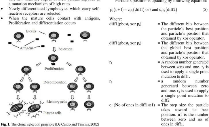
Artificial Immune System inspired by natural immune system in which the human beings and animals are protected (using antibodies) from intrusions by substance (antigens). Clonal Selection is a type of adaptive immune system which is directed against specific antigen and consists of two major types of lymphocytes; B-cells (white blood cells which are responsible for producing antibodies) and T-cells (white blood cells also called cells-receptors, they are responsible for detecting antigens) which are involved in process of identify and removing antigen. The basic idea of Clonal Selection as shown in
Fig. (1) (De Castro and Timmis, 2002) based on the proliferation of activated B-cells that have better matching with specific antigen. Those B-cells can be changed in order to achieve a better matching. Clonal selection algorithm take into consideration, the memory set maintenance, death of cells that can’t recognize antigen or have a bad matching and the ratio between re-selection of the clones and their affinity. The main features of the Clonal Selection theory are (Burnet, 1978):
• The new cells are copies of their parents exposed to a mutation mechanism of high rates
• Newly differentiated lymphocytes which carry self-reactive receptors are selected
• When the mature cells contact with antigens, Proliferation and differentiation occurs
Fig. 1. The clonal selection principle (De Castro and Timmis, 2002)
2. NEW PARTICLE SWARM
OPTIMIZATION WITH IMMUNITY
CLONAL SELECTION ALGORITHM
This section presents the new Binary Particle Swarm Optimization with immunity Clonal Algorithm (NPSOCLA). The algorithm combines a modified Binary Particle Swarm Optimization algorithm, the clonal selection algorithm and subset of random population in the aim to achieve a balance between exploration and exploitation. The proposed algorithm is explained in two parts as follows.
2.1. New Binary Particle Swarm Optimization
(NBPSO)
In the NBPSO, the Position is updated without using the velocity. The particle’s step size toward the best position and the global best position is controlled by using logical operators. The NBPSO works as follows.
2.2. Representation
The population is initialized randomly where each particle (pi) in it represented as a binary position vector.
2.3. Position Update Equation
Particle’s position is updating by following equation:
(
)
(
)
(
)
i 1 1 2 2
p t +1 = c r diff1 or / and c r diff2 (5)
Where:
diff1(pbesti xor pi) = The different bits between the particle’s best position and particle’s position that obtained by xor operator. diff1(gbesti xor pi) = The different bits between
the global best position and particle’s position that obtained by xor operator.
r1 = A random number generated
between zero and one. r1 is used to apply a single point mutation to diff1.
r2 = a random number
generated between zero and one. r2 is used to apply a single point mutation to diff2
c2 (No of ones in diff2/n2) = The step size the particle takes toward its best position. n2 is the number between zero and no of ones in diff2.
or/and = A logical operator used to combine the two terms of Equation (5) in one binary vector (new position) Choosing between use (or) or (and) depends on the type of the problem.
Pseudo Code of new binary particle swarm algorithm:
1. Initialize the position for each particle in the swarm 2. While stopping criteria not met do
3. {
4. For i=1 to n 5. {
6. Calculate fitness value
7. If ( (i - particle) fitness > best position) 8. {
9. best position=i-particle 10. }
11. }
12. Choose the best of all best positions as gbest 13. For i=1 to n
14. {
15. Update particle position according to Equation 5 as follows:
16. Set temp position1 to position
17. Set diff1 to the result of (position xor Pbest) 18. Set c1 to the result of dividing the number of ones
in diff1 by n1 19. For j=0 to C1 20. {
21. If (diff1 current bit==1 and tempposition1 current bit==0)
22. {
23. Set temp position current bit to 1 24. Set c1 to c1-1
25. } 26. }
27. If (r1>0.5) 28. {
29. Flip the value of temp position1 [random bit index] 30. }
31. Repeat the same steps from 17 to 29 with diff2 by set temp position 2 to position
32. Set new position to the result of (tempposition1 xor tempposition2)
33. } 34. }
2.4. Clonal Selection Algorithms
In the new proposed Binary Particle Swarm Optimization with immunity Clonal Algorithm in this study, Clonal Selection Algorithm (CSA) is applied on the best-fit particles when the global best position does not change for (m) times. If the initial population size is P then CSA is applied on N = 10*p/100 best fit particles (Pbests). The number of clones generated is given by the following Equation (6):
(
)
CN =floor α β* (6)
Where:
NC = Total number of particles to be cloned from the current particle
α = Fitness ratio of each particle
β = Cloning index
By varying this parameter, number of Clones can be regulated.
The new set C of NC number of cloned particles are then put through a mutation process in such a way that the best fit clone will have least mutation. This is done by the following Equation (7):
( )
M = floor 1-α * C (7)
Where:
M = Number of bits to be flipped in the cloned particle
α = Fitness ratio of each particle C = Mutating index.
By varying this parameter, number of Mutates can be regulated.
The cloning and mutation applied on the best-fit particles of NBPSO to increase the exploration potential of the algorithm near the vicinity of the fittest particles and distant regions from the less fit particles in the search space.
1. Create a population of the best pbests (best particles) in the swarm population.
2. Create n clones from each particle, where n is proportional to the fitness of the particle.
3. Mutate each clone inversely proportionally to its fitness.
4. Calculate the fitness of the cloned particles. 5. Sort.
6. Pick the best of them to be nominated in the next generation without redundancy.
2.5. New Particle Swarm Optimization with
Clonal
Selection
Algorithm
Outline
(NPSOCLA)
This section shows how new particle swarm optimization, clonal selection algorithm and a subset of new random population are combined together.
Pseudo Code of NPSOCLA:
1. Initialize each particle with random position (Initialize population of P size)
2. Initialize max-n iterations 3. While n<max-n iterations 4. {
5. For i=1: population size 6. {
7. Calculate fitness value 8. }
9. Obtain pbests and gbest
10. If gbest doesn’t change for n times 11. {
12. Go to clonal selection algorithm with the best pbests in the swarm population without redundancy
13. New population(P size) = select the best individuals from (swarm population + New random generating population + the clonal selection population)
14. Go to the new binary particle swarm algorithm 15. }
16. Else
17. Updating each particle position according to equation (5)
18. }
3. EXPERIMENTAL RESULTS
To validate the feasibility and effectiveness of the proposed approach, the proposed algorithm was applied on several instances of 0/1 Multidimensional Knapsack
Problem (0/1MKP) found in (Beasley, 2012). The 0/1 Multidimensional Knapsack Problem is an NP-Hard problem (Garey and Johnson, 1979). It can be defined as follows: there are m knapsacks with maximum Cm capacities. All Knapsacks have to be filled with the same x objects. Each object has P profit and w weight. The weight of the object differs from one knapsack to another. The goal is to maximize the profit without violating constraints. The 0/1 MKP can be formulated as Equation (8 and 9):
n i i i 0 Maximize px
=
∑
(8){ }
nij i j i
i 0
w x C , j 1 .m,
Subject x 0,1
= ≤ = … ∈
∑
(9)The solutions to the 0/1 MKP that are represented as binary vectors may be infeasible because one of the knapsack constraints may be violated in the following two cases:
• When initializing the population with random solutions (Random positions)
• When updating the solutions with Equation (5)
So, each solution must verify the m constrained of the knapsack to be accepted as a feasible solution. In our new algorithm, the following technique is used to convert the infeasible solution to feasible solution based on some ideas from greedy algorithm (Kohli et al., 2004) and Check and Repair Operator (CRO) (Labed et al., 2011) as follows:
1. Calculate the profit ratio Rij = Pi/Wij for every item in every knapsack.
2. Compute the max value of the profit ratio Ri = max {Pj/Wij} for every item.
3. Sort items according to the ascending order of Ri 4. Remove the corresponding item with lowest values
of Ri from the item set. (i.e., the value of corresponding bit which is 1 becomes 0).
5. Repeat Step 4 until a feasible solution is achieved.
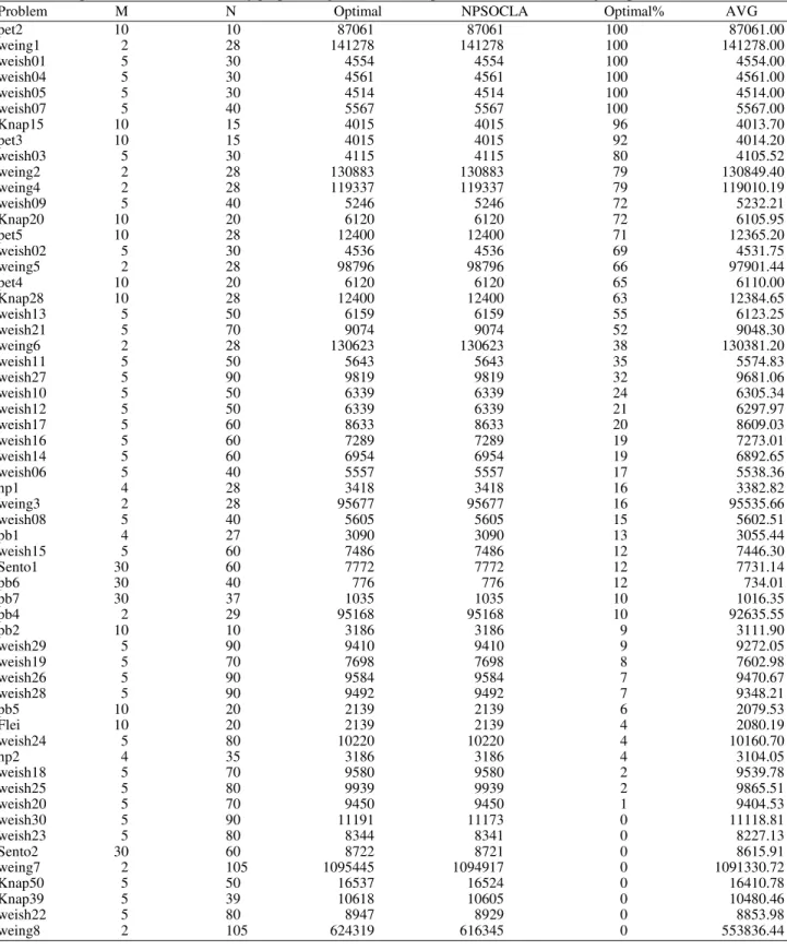
Table 1. Comparison of results obtained by proposed algorithm and the optimal known solution-using or operator
Problem M N Optimal NPSOCLA Optimal% AVG
pet2 10 10 87061 87061 100 87061.00
weing1 2 28 141278 141278 100 141278.00
weish01 5 30 4554 4554 100 4554.00
weish04 5 30 4561 4561 100 4561.00
weish05 5 30 4514 4514 100 4514.00
weish07 5 40 5567 5567 100 5567.00
Knap15 10 15 4015 4015 96 4013.70
pet3 10 15 4015 4015 92 4014.20
weish03 5 30 4115 4115 80 4105.52
weing2 2 28 130883 130883 79 130849.40
weing4 2 28 119337 119337 79 119010.19
weish09 5 40 5246 5246 72 5232.21
Knap20 10 20 6120 6120 72 6105.95
pet5 10 28 12400 12400 71 12365.20
weish02 5 30 4536 4536 69 4531.75
weing5 2 28 98796 98796 66 97901.44
pet4 10 20 6120 6120 65 6110.00
Knap28 10 28 12400 12400 63 12384.65
weish13 5 50 6159 6159 55 6123.25
weish21 5 70 9074 9074 52 9048.30
weing6 2 28 130623 130623 38 130381.20
weish11 5 50 5643 5643 35 5574.83
weish27 5 90 9819 9819 32 9681.06
weish10 5 50 6339 6339 24 6305.34
weish12 5 50 6339 6339 21 6297.97
weish17 5 60 8633 8633 20 8609.03
weish16 5 60 7289 7289 19 7273.01
weish14 5 60 6954 6954 19 6892.65
weish06 5 40 5557 5557 17 5538.36
hp1 4 28 3418 3418 16 3382.82
weing3 2 28 95677 95677 16 95535.66
weish08 5 40 5605 5605 15 5602.51
pb1 4 27 3090 3090 13 3055.44
weish15 5 60 7486 7486 12 7446.30
Sento1 30 60 7772 7772 12 7731.14
pb6 30 40 776 776 12 734.01
pb7 30 37 1035 1035 10 1016.35
pb4 2 29 95168 95168 10 92635.55
pb2 10 10 3186 3186 9 3111.90
weish29 5 90 9410 9410 9 9272.05
weish19 5 70 7698 7698 8 7602.98
weish26 5 90 9584 9584 7 9470.67
weish28 5 90 9492 9492 7 9348.21
pb5 10 20 2139 2139 6 2079.53
Flei 10 20 2139 2139 4 2080.19
weish24 5 80 10220 10220 4 10160.70
hp2 4 35 3186 3186 4 3104.05
weish18 5 70 9580 9580 2 9539.78
weish25 5 80 9939 9939 2 9865.51
weish20 5 70 9450 9450 1 9404.53
weish30 5 90 11191 11173 0 11118.81
weish23 5 80 8344 8341 0 8227.13
Sento2 30 60 8722 8721 0 8615.91
weing7 2 105 1095445 1094917 0 1091330.72
Knap50 5 50 16537 16524 0 16410.78
Knap39 5 39 10618 10605 0 10480.46
weish22 5 80 8947 8929 0 8853.98
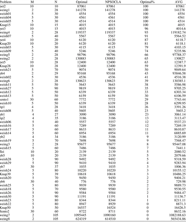
Table 2. Comparison of results obtained by proposed algorithm and the optimal known solution-using and operator
Problem M N Optimal NPSOCLA Optimal% AVG
pet2 10 10 87061 87061 100 87061
weing1 2 28 141278 141278 100 141278
weish01 5 30 4554 4554 100 4554
weish04 5 30 4561 4561 100 4561
weish05 5 30 4514 4514 100 4514
Knap15 10 15 4015 4015 100 4015
pet3 10 15 4015 4015 96 4014.6
weing4 2 28 119337 119337 93 119182.74
weish07 5 40 5567 5567 91 5564.52
pet4 10 20 6120 6120 87 6118.7
Knap20 10 20 6120 6120 81 6118.1
weish03 5 30 4115 4115 79 4103.15
weish09 5 40 5246 5246 74 5235.96
weing5 2 28 98796 98796 66 97788.37
weing2 2 28 130883 130883 65 130827
pet5 10 28 12400 12400 63 12387.7
Knap28 10 28 12400 12400 59 12391.9
weish21 5 70 9074 9074 50 9049.64
pb4 2 29 95168 95168 43 93846.58
weish02 5 30 4536 4536 41 4516.38
weing6 2 28 130623 130623 39 130385.1
weish11 5 50 5643 5643 38 5586.98
weish27 5 90 9819 9819 35 9705.25
weish12 5 50 6339 6339 33 6303.34
weish13 5 50 6159 6159 30 6106.59
sento1 30 60 7772 7772 29 7743.44
weish10 5 50 6339 6339 28 6299.95
hp1 4 28 3418 3418 26 3391.26
weish08 5 40 5605 5605 23 5603.2
pb1 4 27 3090 3090 23 3061.14
hp2 4 35 3186 3186 13 3113.47
weish06 5 40 5557 5557 12 5537.23
weish16 5 60 7289 7289 12 7269.19
weish17 5 60 8633 8633 11 8610.87
weish14 5 60 6954 6954 11 6885.69
pb2 4 34 3186 3186 9 3120.99
weish19 5 70 7698 7698 9 7568.47
weing3 2 28 95677 95677 8 95447.08
weish15 5 60 7486 7486 7 7441.1
flei 10 20 2139 2139 5 2080.52
pb5 10 20 2139 2139 5 2079.66
weish28 5 90 9492 9492 5 9318.59
weish29 5 90 9410 9410 4 9283.94
pb7 30 37 1035 1035 3 1006.36
weish24 5 80 10220 10220 3 10155.12
Knap39 5 39 10618 10618 3 10486.25
weish20 5 70 9450 9450 2 9404.21
pb6 30 40 776 776 2 729.98
weish25 5 80 9939 9939 2 9889.73
weish18 5 70 9580 9580 2 9530.55
weish26 5 90 9584 9584 2 9484.47
weish30 5 90 11191 11191 1 11136.7
weish23 5 80 8344 8344 1 8211.11
weish22 5 80 8947 8929 0 8871.3
Knap50 5 50 16537 16524 0 16426.5
Sento2 30 60 8722 8711 0 8632.16
weing7 2 105 1095445 1090160 0 1082188.63
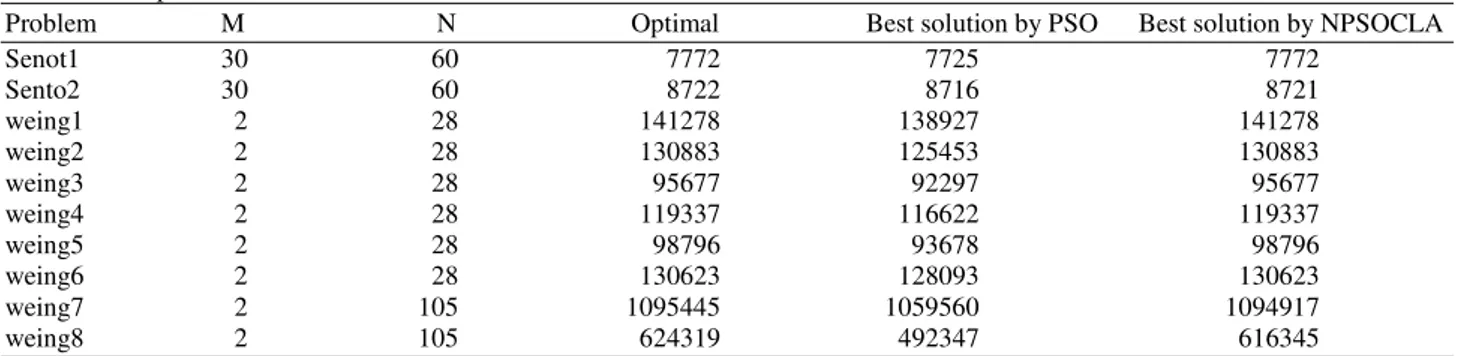
Table 3. Comparative results between PSO and NPSOCLA
Problem M N Optimal Best solution by PSO Best solution by NPSOCLA
Senot1 30 60 7772 7725 7772
Sento2 30 60 8722 8716 8721
weing1 2 28 141278 138927 141278
weing2 2 28 130883 125453 130883
weing3 2 28 95677 92297 95677
weing4 2 28 119337 116622 119337
weing5 2 28 98796 93678 98796
weing6 2 28 130623 128093 130623
weing7 2 105 1095445 1059560 1094917
weing8 2 105 624319 492347 616345
Table 4. Comparative results between PSO and NPSOCLA Probleminstance GA NPSOCLA --- --- --- Name Optimum Average #Max Average #Max knap15 4015 4012.70 83 4015.00 100 knap20 6120 6102.30 33 6118.10 81 knap28 12400 12374.70 33 12384.65 63 knap39 10618 10536.90 4 10486.25 3 knap50 16537 16378.00 1 16426.50 0
Fig. 2. A comparison between PSO and NPSOCLA explains the percent of finding the optimal solution
Two parts of experiments were performed. First, the proposed algorithm was tested when the logical operator in Equation (5) is (or) and when it is (and). In the second part of experiments, the obtained results were compared with the obtained solutions in (Khuri et al., 1994; Hembecker et al., 2007).
Table 1 and 2 show the experiment result of the proposed algorithm with some instances taken from ORlib (Beasley, 2012). The first column indicates the name of problem. The second column indicates the number of knapsacks (M). The third column indicates the number of objects (N). The fourth column indicates the best-known solution. The fifth column indicates the best result obtained by the New Particle Swarm Optimization with Clonal Selection algorithm. The sixth
column indicates the number of times that the New Particle Swarm Optimization with Clonal Selection algorithm reaches the best-known solution (#max). The seventh column indicates the average obtained over all 100 runs by (NPSOCLA).
We can deduce from Table 1 and 2 that, the NPSOCLA found the optimum solution for 53 of the 58 test cases. It should be noted that there are five problems (sento2, knap50, weish22, weing7, weing8) that do not reach the optimum solution but are very close to it.
Table 3 andFig. 2 show a comparison in terms of
best solution between the exact solutions (optimal), proposed algorithm and PSO algorithm (Hembecker et al., 2007). It is show that the NPSOCLA outperforms the PSO algorithm.
Table 4 shows a comparison between a GA in
(Khuri et al., 1994) and the New Particle Swarm Optimization with Clonal Selection Algorithm (NPSOCLA). The first two columns (problem instance) report the name of the problem and the maximum obtainable benefit. The following groups of columns report the results archived by GA in (Khuri et al., 1994) and by NPSOCLA, respectively. We show the average profit obtained over all 100 runs and, in the column #max, the number of times the best solution is reached. It is show that the NPSOCLA outperforms the GA in kanp15, knap20 and, knap28 .The GA outperforms the proposed algorithm in knap39. In knap50 the GA reach the optimal solution one time but its average is less than the NPSOCLA’s average, which doesn’t reach the optimal solution.
4. CONCLUSION
(NPSOCLA) has a good performance; on the other hand the difficult task in the proposed algorithm is to choose the proper parameters because the best setting for parameters can be different from problem to another So, our fundamental outlook moving towards design a self-adaptive method to control parameters setting.
5. REFERENCES
Beasley, J.E., 2012. OR-Library-Operations Research Library.
Burnet, F.M., 1978. Clonal Selection and After. In: Theoretical Immunology, Bell, G.I., A.S. Perelson and G.H. Pimbley (Eds.), Marcel Dekker Inc., pp: 63-85.
De Castro, L.N. and J. Timmis, 2002. Artificial immune systems: A new computational intelligence approach. Springer, 1: 57-58.
Eberhart, R. and J. Kennedy, 1995. A new optimizer using particle swarm theory. Proceedings of the 6th International Symposium on Micro Machine and Human Science, Oct. 4-6, IEEE Xplore Press,
Nagoya, pp: 39-43. DOI:
10.1109/MHS.1995.494215
Engelbrecht, A.P., 2005. Fundamentals of Computational Swarm Intelligence. 1st Edn., John Wiley and Sons, Chichester, ISBN-10: 0470091916, pp: 672.
Garey, M.R. and D.S. Johnson, 1979. Computers and Intractability: A Guide to the Theory of NP-Completeness. 10th Edn., W. H. Freeman, New York, pp: 338.
Gherboudj, A. and S. Chikhi, 2011. BPSO algorithms for knapsack problem. Proceedings of the 3rd International Conference on Recent Trends in Wireless and Mobile Networks, Jun. 26-28, Springer Berlin Heidelberg, Ankara, Turkey, pp: 217-227. DOI: 10.1007/978-3-642-21937-5_20
Gherboudj, A., S. Labed and S. Chikhi, 2012. A new hybrid binary particle swarm optimization algorithm for multidimensional knapsack problem. Proceedings of the 2nd International Conference on Computer Science, Engineering and Applications, May 25-27, Springer Berlin Heidelberg, New Delhi, India, pp: 489-498. DOI: 10.1007/978-3-642-30157-5_49
Hembecker, F., H.S. Lopes and W. Godoy Jr., 2007. Particle swarm optimization for the multidimensional knapsack problem. Proceedings of 8th International Conference on Particle Swarm Optimization for the Multidimensional Knapsack Problem, Apr. 11-14, Heidelberg Springer-Verlag, Warsaw, Poland, pp: 358-365. DOI: 10.1007/978-3-540-71618-1_40
Kennedy, J. and R.C. Eberhart, 1997. A discrete binary version of the particle swarm algorithm. Proceedings of the IEEE International Conference on Systems, Man and Cybernetics, Oct. 12-15, IEEE Xplore Press, Orlando, FL., pp: 4104-4108. DOI: 10.1109/ICSMC.1997.637339
Kennedy, J., R.C. Eberhart and Y. Shi, 2001. Swarm Intelligence. 1st Edm., Morgan Kaufmann, San Francisco, Calif, USA.
Khanesar, M.A., M. Teshnehlab and M.A. Shoorehdeli, 2007. A novel binary particle swarm optimization. Proceedings of the 15th Mediterranean Conference on Control and Automation, Jun. 27-29, IEEE Xplore Press, Athens, pp: 1-6. DOI: 10.1109/MED.2007.4433821
Khuri, S., T. Back and J. Heitkotter, 1994. The zero/one multiple knapsack problem and genetic algorithms. Proceedings of the ACM Symposium on Applied Computing, (SAC’ 94), ACM Press, Phoenix, Arizona, USA., pp: 578-582. DOI: 10.1145/326619.326694
Kohli, R., R. Krishnamurti and P. Mirchandani, 2004. Average performance of greedy heuristics for the integer knapsack problem. Eur. J. Operat. Res., 154: 36-45. DOI: 10.1016/S0377-2217(02)00810-X Labed, S., A. Gherboudj and S. Chikhi, 2011. A
modified hybrid particle swarm optimization algorithm for multidimensional knapsack problem. Int. J. Comput. Applic., 34: 11-16. DOI: 10.5120/4070-5586
Mohamad, M.S., S. Omatu, S. Deris and M. Yoshioka, 2011. A modified binary particle swarm optimization for selecting the small subset of informative genes from gene expression data. IEEE Trans. Inform. Technol. Biomed., 15: 813-822. DOI: 10.1109/TITB.2011.2167756
Shi, Y. and R. Eberhart, 1998. A modified particle swarm optimizer. Proceedings of the IEEE International Conference on Evolutionary Computation, May 4-9, IEEE Xplore Press, Anchorage, AK., pp: 69-73. DOI: 10.1109/ICEC.1998.699146