Performance Analysis of Transfer function Based Active Noise Cancellation Method Using Evolutionary Algorithm

(1)

International Journal of Electronics Communication and Computer Engineering Volume 5, Issue 1, ISSN (Online): 2249_–071X, ISSN (Print): 2278_–4209

Performance Analysis of Transfer function Based Active

Noise Cancellation Method Using Evolutionary

Algorithm

Prof. Vikas Gupta, Prof. Ritu Chauhan, Kumkum Dubey

Abstract – Due to the exponential increase of noise pollution, the demand for noise controlling system is also increases. Basically two types of techniques are used for noise cancellation active and passive. But passive techniques are inactive for low frequency noise, hence there is an increasing demand of research and developmental work on active noise cancellation techniques. In this paper we introduce a new method in the active noise cancellation system. This new method is the transfer function based method which used Genetic and Particle swarm optimization (PSO) algorithm for noise cancellation. This method is very simple and efficient for low frequency noise cancellation. Here we analysis the performance of this method in the presence of white Gaussian noise and compare the results of Particle swarm optimization (PSO) and Genetic algorithm. Both algorithms are suitable for different environment, so we observe their performance in different fields. In this paper a

comparative study of Genetic and Particle swarm

optimization (PSO) is described with proper results. It will go in depth what exactly transfer function method, how it work and advantages over neural network based method.

Keywords–Active Noise Control, Genetic, Particle Swarm

Optimization, Transfer Function.

I. I

NTRODUCTION

Present days high speed & quality is a major issue in communication. Lots of techniques are developed for improving the quality of signal in communication field. For proper communication, it is necessary that information is received at the receiver without any distortion. But due to the presence of noise distortion take place. For transmission of acoustic signal this distortion is not tolerable. For removing distortion it is necessary that noise will be cancelled out. Different methods are used for cancelling the noise one of the famous method is active noise control (ANC) method. In ANC method an antinoise signal is generated, whose magnitude is similar to the noise signal but its phase is opposite to the noise signal. When antinoise and noise signal are combined then destructive interference take place and noise is cancelled out. This scheme contains a reference microphone which sampled noise to be cancelled, an electronic control unit to process the input signal and generate control signal. This control signal is given to the loudspeaker and finally loudspeaker generate antinoise signal and antinoise signal get mixes with noise signal and cancelled it. If some noise is remaining out then it is treated as an error signal and it is absorbed by the microphone it act as feedback signal to the controller. The controller can adjust itself for generating such type of antinoise signal so that it can cancelled out noise completely and error become zero. Controller contain digital filter which synthesis the

antinoise signal. The performance of digital filter is affected by the type of filter, filter weight values are adjusted by using different algorithm. Large numbers of algorithms are developed for cancellation of noise. Like LMS, Filtered-X LMS algorithm, FLANN etc. LMS is one of the simplest algorithm but its convergence speed is low. So that it is updated and filtered-X LMS algorithm is used for removing noise of linear environment. But these methods are not suitable for non-linear environment, hence other methods were developed for non-linear environment these include volterra series, memory polynomial filters, FLANN filter etc. FLANN is one of the successful methods for non-linear environment. But this method increases computation complexity of the system. For removing the limitation of FLANN, genetic algorithm is used with it. Genetic algorithm and PSO algorithm are the best algorithm for removing noise. Since their convergence speed is high in comparison to other algorithm and they remove the requirement of secondary path thus complexity in computation reduces. In this we

don’t use neural network. Here noise is calculated from

transfer function of channel. This is a simplest method for calculating noise. It can measure accurately and fastly. Since neural network is a complex method, so make it simple transfer function method is used.

II. A

DAPTIVE

A

LGORITHM

(2)

III. E

VOLUTIONARY

A

LGORITHM

These algorithms [2] are stochastic search methods that mimic the metaphor of natural biological evolution. Evolutionary algorithm based method are used in communication system for channel equalization, ANC system. This algorithm based on the principal of survival of the fittest to produce better and better approximations to a solution. At each generation a new set of approximations is created by the process of selecting individual according to their level of fitness in the problem domain and combine them together for generating new individuals. This process leads to the evolution of population of individual that are better suited to their environment. Evolutionary algorithms involve selection, recombination, migration, locality selection and neighborhood. At the beginning a number of individual are randomly initialized. The objective function is then evaluated for these individuals and the initial generation is produced. If the optimization criteria are not met the creation of new generation starts. Individuals are selected according to their fitness for the production of off-spring . Parents are recombined to production off-spring. All offspring will be mutated with a certain probability. The fitness of the offspring is then computed .The offspring are inserted into the population replacing the parents, producing a new generation. This cycle is performed until the optimization criteria is reach. It contain following

algorithms:-A. Genetic Algorithm

This is the most popular type of evolutionary algorithm. Genetic algorithm is based upon the process of natural

selection and doesn’t require gradient statistics. This

algorithm is able to find a global error minimum. The genetic algorithm with small population size and high mutation rates can find a good solution fastly. This algorithm is started with a set of solution called population. Solution from one population are taken and used to form a new population. The new population is better than old population. Solutions which are selected to form new solutions are selected according to their fitness. This process is repeated until some condition is satisfied. In genetic algorithm, a population is evolved toward better solution. Each individual solution has a set of properties which can be mutated and altered, solution are represented in binary as string of 0s and 1s. The process of randomly generated population at the starting of algorithm is known as iteration or generation. Finally it involved all the steps of evolutionary algorithm that means selection of individual on the basis of fitness value and then replacement of old individual until the optimum solution is achieved.

Limitation:-1. Evaluation of fitness function for complex problem is complicated. Finding the optimal solution to complex high dimensional, multimodal problems require very expensive fitness function evaluation.

2. Genetic algorithm is not suitable for complex function. especially when the number of elements which are exposed to mutation is large.

3. Genetic algorithm may have a tendency to converge towards local optima or rather than the global optimum of the problem.

B. Particle swarm optimization

It was first developed in 1995 by Eberhart and Kennedy [15] rooted on the notion of swarm intelligence of insects, birds etc. This algorithm attempts to mimic the natural process of group communication of individual knowledge that occurs when such swarms, flock, migrate, forage etc. in order to achieve such optimum property such as configuration or location. PSO algorithm cannot be directly used in the ANC system as the performance of the algorithm depends on a set of error samples and not on the instantaneous value of the error microphone. In addition the conventional PSO based optimization, the same data set is used to the particles respectively in every generation. The objective of the PSO based ANC algorithm is to minimize the mean square error that is sensed by the error microphone. Let us consider a coefficient vector of P adaptive filters as population which is represented as a set of particles in the PSO terminology. The PSO algorithm is initialized with a population of random solutions. In this case the coefficient vectors of the P adaptive filters are used as the initial random solutions. Let this set be represented as

(3)

symbol gbest and its position is represented as wgbest. The PSO algorithm updates the velocity and position of each particle toward its wpbestand wgbestpositions at each step according to the following update

equations:-vi(k)= vi(k-1) + r1[wpbesti–wi(k)]+ r2 [wgbest–wi(k)]. Wi(k) = wi(k-1) + vi(k)

Where r1 and r2 are two random numbers that are generated independently in the range [0,1]. The basic PSO algorithm uses two random vectors for r1 and r2; however we use r1 and r2 as random numbers instead , due to reduced complexity. Vi(k) is a new velocity for each particle based on its previous velocity vi(k-1), the

particle’s position at which the best fitness has been

achieved wpbest and the best positions of each particle achieved so far among the neighbors wgbest.

Advantages of

PSO:-1. PSO has memory i.e. every particle remembers its best solution aswell as the group’s best solution.

2. Its initial population is maintained fixed throughout the execution of the algorithm and so there is no need for applying operators to the population.

3. This process is both time & memory storage consuming.

4. Another key advantage of PSO is the ease of implementation in both the contest of coding and parameter selection.

Limitations

1. If the new gbest particle is an outlying particle with respect to the swarm, the rest of the swarm can tend to move toward the new gbest from the same direction. 2. Particles closer to gbest will tend to quickly converge

on it and become stagnant while the other more distant particles continue to search. A stagnant particle is essentially useless because its fitness continues to be evaluated but it no longer contributes to the search.

IV. P

ROPOSED

M

ETHODOLOGY

Transfer function is measured here for calculating noise. For measuring transfer function a pilot signal is sent through the channel and then ratio of fourier transform of input signal and output signal is calculated that gives us transfer function of the channel. Thus by calculating the

transfer function we calculate the behavior of channel. We follow the change occur in the behavior of channel through its transfer function. This change is take place due to noise effect.

Noise at observed microphone = Transfer function noise to Observed microphone*noise signal.

Noise at error microphone = Transfer function noise to error microphone* noise signal.

After calculating noise from transfer function we find out the difference between the noise and antinoise signal. If noise is not fully cancelled by antinoise signal then coefficients of PSO algorithm are updated so that it generate such type of antinoise signal which cancel the noise completely.

V. R

ESULTS

A. Effect of Generations

From experimental results we obtain table 1 between MSE, calculated time and total generations, which show that at the starting level when we increase generations then MSE value also increases i.e. from 100 to 500 MSE increases. However, when more samples are collected M.S.E. tends to decrease, M.S.E. decreases over generations i.e. for very high generations like 700, 1000 MSE decreases.

Table 1: Computation time & MSE of PSO for different generations

S.No. Total

Generations

Calculated Time

MSE

1 100 0.99226 0.0031235

2 200 0.95521 0.0033901

3 500 1.176 0.0036691

4 700 0.9799 0.003609

5 1000 1.0873 0.0032433

B. Comparison of PSO and genetic

Both methods are efficient for anti noise cancellation but for different environment and for different parameters. Genetic is suitable for discrete variable and PSO is suitable for continuous variable.

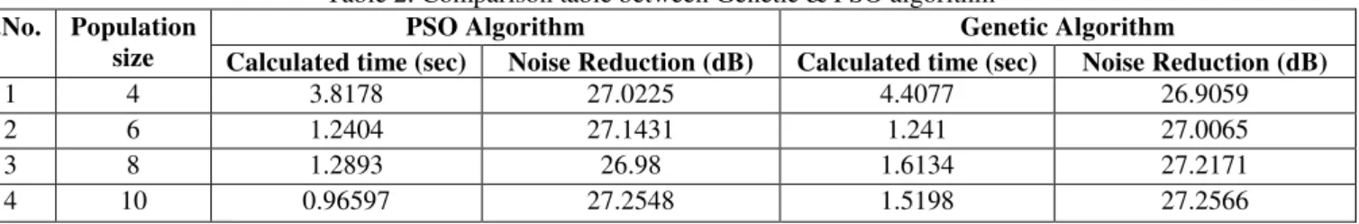
Table 2: Comparison table between Genetic & PSO algorithm S.No. Population

size

PSO Algorithm Genetic Algorithm

Calculated time (sec) Noise Reduction (dB) Calculated time (sec) Noise Reduction (dB)

1 4 3.8178 27.0225 4.4077 26.9059

2 6 1.2404 27.1431 1.241 27.0065

3 8 1.2893 26.98 1.6134 27.2171

4 10 0.96597 27.2548 1.5198 27.2566

From the table 2 it is clear that PSO converge fastly than genetic algorithm because calculated time of PSO is lower than genetic. But some time noise reduction level of PSO

is high and some time genetic. Since it can’t we say that

which algorithm is best because the efficiency of both algorithm depend on the population size, generations, noise environment etc.

(4)

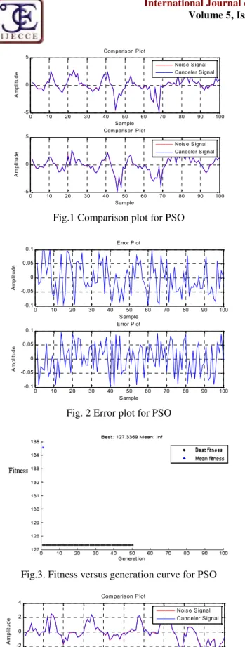
C Fig.1 Comparison plot for P

Fig. 2 Error plot for PSO

Fig.3. Fitness versus generation cu

Fig.4. Comparison Plot for Ge

0 10 20 30 40 50 60 70 80 90 100

-5 0 5 Sam ple A m p li tu d e

Com parison Plot

Noise Signal Canceler Signal

0 10 20 30 40 50 60 70 80 90 100

Com parison Plot

0 10 20 30 40 50 60 70 80 90 100

-0.1 -0.05 0 0.05 0.1 Sample A m p li tu d e Error Plot

0 10 20 30 40 50 60 70 80 90 100

-4 -2 0 2 4

S am ple

A m p li tu d e

Com paris on P lot

Nois e S ignal Canc eler S ignal

0 10 20 30 40 50 60 70 80 90 100

-5 0 5

S am ple

A m p li tu d e

Com paris on P lot

SO

curve for PSO

r Genetic

Where as in figure 4,5,6 the c fitness curve for Genetic alg population size is 8, total gene time is 4.7846 sec, MSE 0.003 and speakers is 2 and noise red Here comparison plot show the and canceller signal.

Fig.5. Error plot

Fig.6. Fitness curv

VI. C

ONCL

Finally we concluded that ca simple in industries if we calcu without using any neural netwo out the approximate value of n antinoise signal which cancelle suitable for removing non-line plot, comparison plot and fitnes PSO work more efficiently a genetic.

R

EFERENCE

[1] S. U. H. Qureshi, “Adaptive E

1349–1387, September 1985 [2] D. E. Goldberg, Genetic Algo

and Machine Learning, Addison [3] C. Y. Chang and D. R. Chen, “

secondary path identification algorithm IEEE Trans. Instrum 2327, Sep. 2010.

0 10 20 30 40 50 60 70 80 90 100

Com parison Plot

0 10 20 30 40 50 60 70 80 90 100

Com parison Plot

0 10 20 30 40 50 60 70 80 90 100

-4 -2 0 2 4

S am ple

A m p li tu d e

Com paris on P lot

0 10 20 30 40 50 60 70 80 90 100

-5 0 5

S am ple

A m p li tu d e

Com paris on P lot

0 10 20 30 40 50 60 70 80 90 100 -0.1 -0.05 0 0.05 0.1 Sample A m p li tu d e Error Plot

e comparison plot, error plot, algorithm is given, where enerations is 100, calculated 031927, no. of error sensors eduction level is 27.2577 dB. he comparison between noise

lot for Genetic

urve for Genetic NCLUSION

cancellation of noise is very lculated its transfer function twork method we easily find f noise and then generate its elled it. This method is very inear distortions. From error itness curve it is also clear that and converge fastly than

RENCES

e Equalization,” IEEE, vol. 73, pp.

lgorithms in Search, Optimization, ison-Wesley, 1989..

, “Active noise cancellation without

on by using an adaptive genetic um. Meas., vol. 59, no. 9, pp. 2315– 0 10 20 30 40 50 60 70 80 90 100 -0.1 -0.05 0 0.05 0.1 Sample A m p li tu d e Error Plot

(5)

[4] S. C. Douglas, “Fast implementations of the filtered-X LMS and

LMS algorithms for multichannel active noise control,” IEEE Trans. Speech Audio Process., vol. 7, no. 4, pp. 454–465, Jul. 1999.

[5] S. M. Kuo and D. R. Morgan,Active Noise Control Systems— Algorithms and DSP Implementations. New York: Wiley, 1996. [6] C. A. Jacobson, C. R. Johnson, D. C. McCormick, and W. A.

Sethares, “Stability of active noise control algorithms,” IEEE Signal Process. Lett., vol. 8, no. 3, pp. 74–76, Mar. 2001. [7] M. Diego, A. Gonzalez, M. Ferrer, and G. Pinero, “An adaptive

algorithms comparison for real multichannel active noise

control,” in Proc. 12th Proc. Eur. Signal Process. Conf., Sep. 2004, pp. 925–928.

[8] M. Young, The Technical Writer’s Handbook. Mill Valley, CA:

University Science, 1989.

[9] John G. Proakis, Dimitris G. Manolakis, “Digital Signal Preocessing”, Pearson Publication, 2007.

[10] S. M. Kuo and D. R. Morgan, Active noise control systems: Algorithms and DSP implementations. New York: Wiley, 1996. [11] L. Yao and W. A. Sethares, “Nonlinear parameter estimation via

the genetic algorithm,”IEEE Transactions on Signal Processing, vol. 42, April 1994.

[12] S.J. Elliott and P.A. Nelson. Active noise control. IEEE signal processing magazine, pages 12–35, October 1993.

[13] P. L. Feintuch, N. J. Bershad and A. K. Lo, “A frequency -domain model for filtered LMS algorithms - Stability analysis,

design, and elimination of the training mode,” IEEE Transactions on Signal Processing, vol. 41, pp. 1518-1531, Apr. 1993.

[14] D.R Morgan. An analysis of multiple correlation cancellation loops with a filter in the auxiliary path. IEEE Transactions on Acoustics, Speech and Signal Processing, ASSP-28(4):454–467, August 1980.

[15] R. C. Eberhart and J. Kennedy, “A new optimizer using particle

swarm theory,” Proceedings of the Sixth International

Symposium on Micromachine and Human Science, Nagoya, Japan. pp. 39–43, 1995.

A

UTHOR

’

S

P

ROFILE

Vikas Gupta

is currently Professor in Electronics and Communication department and working as HOD in E.C. department, Technocrats Institute of Science and Technology college, Bhopal. He had been completed his B.E. in Electronics & Communication branch and M.Tech. in Digital Communication and Pursuing Ph.D. from MANIT, Bhopal

Ritu Chauhan

is currently working as a Professor in Electronics and Communication department, Technocrats Institute of Science & Technology college, Bhopal. She had completed her B.E. in Electronics & Communication branch from MPCT College Gwalior and MTech in Communication Control & Networking from MITS college Gwalior.