Analyzing the Long Term Cohesive Effect of
Sector Specific Driving Forces
Yonatan Berman1*, Eshel Ben-Jacob1†, Xin Zhang2, Yoash Shapira1*
1School of Physics and Astronomy, Tel-Aviv University, Tel-Aviv, Israel,2College of Transport and Communication, Shanghai Maritime University, Shanghai, China
†Deceased.
*yonatanb@post.tau.ac.il(YB);yoashshapia@gmail.com(YS)
Abstract
Financial markets are partially composed of sectors dominated by external driving forces, such as commodity prices, infrastructure and other indices. We characterize the statistical properties of such sectors and present a novel model for the coupling of the stock prices and their dominating driving forces, inspired by mean reverting stochastic processes. Using the model we were able to explain the market sectors’long term behavior and estimate the coupling strength between stocks in financial markets and the sector specific driving forces. Notably, the analysis was successfully applied to the shipping market, in which the Baltic dry index (BDI), an assessment of the price of transporting the major raw materials by sea, influences the shipping financial market. We also present the analysis of other sectors—the gold mining market and the food production market, for which the model was also success-fully applied. The model can serve as a general tool for characterizing the coupling between external forces and affected financial variables and therefore for estimating the risk in sec-tors and their vulnerability to external stress.
Introduction
As a part of the effort to study financial markets, sectors within the market, in which stocks are strongly interacting are particularly analyzed [1–10]. Due to their nature, some of these sectors are affected by external driving forces. For example, the energy sector stocks are strongly affected by the oil and natural gas prices. Such sectors are expected to differ in various aspects from the market index, due to their dependence on external forces. Analyzing the behavior of such sectors is meaningful for the overall understanding of the stock market. In particular, the importance of such sectors is relevant due to their role in diversifying the market, by incorpo-rating information on external indices and forces [7–9,11–14].
The aim of this paper is to characterize the statistical properties of sectors in the context of their coupling with external driving forces. The characterization is accompanied by proper modeling of this coupling, resulting in the cointegration of the stock prices and the driving forces, as well as in Granger causality between the index and the stock prices [15,16]. Using the model, it is possible to estimate the coupling strength between the external forces and the
OPEN ACCESS
Citation:Berman Y, Ben-Jacob E, Zhang X, Shapira Y (2016) Analyzing the Long Term Cohesive Effect of Sector Specific Driving Forces. PLoS ONE 11(3): e0152487. doi:10.1371/journal.pone.0152487
Editor:Wei-Xing Zhou, East China University of Science and Technology, CHINA
Received:October 1, 2015
Accepted:March 15, 2016
Published:March 31, 2016
Copyright:© 2016 Berman et al. This is an open access article distributed under the terms of the Creative Commons Attribution License, which permits unrestricted use, distribution, and reproduction in any medium, provided the original author and source are credited.
Data Availability Statement:Data are available from the following sources: 1. Yahoo! Finance (http:// finance.yahoo.com). Data taken from Yahoo! Finance include all stock prices used as well as the NASDAQ index and gold prices. 2. Clarkson’s database (http:// sin.clarksons.net). The Baltic dry index historical values were taken from this database. 3. NASDAQ financial database (http://www.nasdaq.com/markets/ wheat.aspx). This database was used to determine historical wheat prices.
stock prices in addition to estimating the risk in specific sectors and assessing their vulnerabil-ity to external stress.
First, we devise a theoretical model for a set of random walking stocks coupled to an exter-nal force or index. We then aexter-nalyze the statistical properties of the shipping sector, as a typical example of a sector in the financial market, and compare the model results with these statistical properties. In order to further validate the model, it is applied to the gold mining and food pro-duction sectors as well. Finally, a discussion of the results and a summary of the work are presented.
A coupling model for a market sector with an external driving force
As an initial step, we devise a theoretical model for the behavior of a set of stocks with an exter-nal driving force. The main ratioexter-nale behind the model is the market mechanism, sometimes apparent in fundamental and technical analysis, in which prices of indices and various other variables are treated as indicators for future outcome. On the daily level, the change of each stock can be treated as random, added by a coupling term, which prevents the stock price from significantly diverging on the long run from the driving force. This mechanism produces an effective interaction between the stocks, creating a process of cointegration as well as Granger causality between the stock prices and the index.Assuming the external driving force is a time seriesIt, witht= 1,. . .,N, we produceMtime
series for the price ofMstocks, denoted asXi
t, withi= 1,. . .,M. We arbitrarily set the initial
price of each stock to be 1, and assume, without the loss of generality, thatI1= 1. We randomly
create a set of random noise seriesoit, which followNð0;0:0001Þand define fort>1:
Xi t¼X
i
t 1 1þo i t
þZi It 1 X i t 1
; ð1Þ
whereηiis defined as the strength of the coupling between thei-th stock andIt.
We assume the random setsoitare independent and identically distributed. For results
dem-onstrating the weak effect of this correlation, the reader is referred toS1 Fig.
In order to investigate the results of the model, we initially use a randomwalk to representIt.
Given thatI1= 1,It¼ Qt
j¼21þj, where for eachj,jfollowsNð0;0:0001Þ. The choice in this
specific statistical noise for the daily return and the daily relative change of the index is origi-nated in the typical mean and standard deviation of the return distribution of several external indices (such as the Baltic Dry Index and the gold price). In practice, the distribution is not normal, however, a more realistic distribution will not affect the model results significantly (see
S2 Figfor additional information).
A typical result of the model for a randomItwith 4 randomly generated stocksXit(i= 1, 2,
3, 4) is presented inFig 1for 2000 days and for 2 values of coupling strength—0.01 and 0 (we considered the couplingηito be independent ofiin this case). It is clearly visible that forη= 0,
the stocks do not follow the trend of the driving forceIt, and in this case the average correlation
between the stock prices andItis 0.06. Thefigure shows one typical realization of the model.
Averaging over a large number of realizations would produce a price correlation matrix, which is similar to matrices E and F, since the correlation between the different stock prices andIt
would go to zero. This similarity was tested using aχ2test, considering 5 degrees of freedom
(since there are 5 independent time series) and taking the matrix F as the expected matrix. The averaged price correlation matrix forη= 0 and 1000 realizations of the model serves as a good
fit to the single realization correlation matrix F withp<0.01.
Forη= 0.01, the stocks follow the external force trend and a narrower“braid”is obtained.
In this case, the average correlation between the stock prices andItwas 0.86. The correlation
between the daily change of the external force and the stocks was also calculated. In both cases
design, data collection and analysis, decision to publish, or preparation of the manuscript.
Competing Interests:The authors have declared
Fig 1. A typical result for the coupling model.A randomwalk was used asIt(thick blue curve), and following the coupling model, the prices of 4 stocks
it was very low, and practically insignificant: 0.01 forη= 0 and -0.01 forη= 0.01. In addition,
the correlation between the modeled stock prices and a randomwalk was 0 on average, as expected, independent of the value ofη.
The results for the caseη= 0.01, depicted inFig 1, demonstrate that a substantial correlation
exists between the stock prices and the index, while the returns are practically uncorrelated. In other words, we obtain a“cohesive”effect of the driving force on the sector stocks in the long run. This behavior is the kind of behavior we would also expect from sectors and their appro-priate external driving forces [17–22].
The modeled stock prices produced demonstrate the property of cointegration. We used the Engle-Granger cointegration test [23] to estimate whether the stock prices andItmeet this
property. Depending onη, the stock prices analyzed were found as cointegrated with each
other, as well as cointegrated withIt(withp<0.01). Forη= 0, the stock prices are not
cointe-grated (p>0.01). Hence, for proper modeling of sectors and their driving forces, in which the
stock prices are cointegrated,ηshould be large enough. We point out that cointegration is not
a continuous quantitative property such as correlation, and the cointegration property is neces-sary but not sufficient. In addition, we use the Granger causality test in order to test the rela-tionship between the different time series produced. While other measures of similarity can be also used [24–26], we would mainly use correlation as the continuous quantitative measure to evaluate the similarity between the model results and the real data. We note that the similarity between the external driving forces and the price of a certain stock is more profound than only being strongly correlated. However, within the scope of this work, we reduce the discussion to correlation, cointegration and Granger causality.
The only parameter in the model isη, the coupling intensity. It is responsible for the
result-ing correlation between the stock prices and the external force. In order to test its effect on this correlation, the dependence of the average correlation between the force and the stock prices was calculated. The results are presented inFig 2. They demonstrate that asηincreases, the
average correlation increases, with an asymptotic value at 1. The actual values inFig 2weakly depend on the variance ofIt, while a thorough discussion of the quantitative effects of the
vari-ance and other statistical attributes of the external driving forces are left for future work.
Single factor and mean reverting models in finance
The derivation of the model, described previously, is based on the explained rationale regarding the effect of external driving forces on investors’decision making, hence on the prices of stocks in various sectors. The resulting model, formulated inEq (1), is reminiscent of the broad family of single factor models, used extensively in various fields of finance [27–29]. However, these models differ fundamentally fromEq (1), most importantly by modeling the dynamics of stock prices directly. Usually, single factor models are used for modeling return and interest rates and incorporate linear rather than non-linear dynamics.
Another type of model, to which the derived model is very similar, is a mean reversion model type [30]. These models, of which some are also single-factored, are extensively used in various fields such as physics, meteorology and finance. Their financial application is usually for modeling interest rates [28,31], but also other financial variables characterized by significant positive or negative autocorrelation [32]. A basic discrete mean reverting model inspired by the Ornstein-Uhlenbeck process, a prototype of mean reverting processes, is the following [30]:
Xt Xt 1¼Z mð Xt 1Þ þsðWt Wt 1Þ; ð2Þ
whereμ,ηandσare parameters andWtis a standard Brownian motion (we will refer toEq (2)
The similarity of this process toEq (1)is clear, however, in this standard version of the pro-cess,μis usually considered as constant. If we letμchange in time (It), it becomes almost
iden-tical toEq (1), given thatσis taken as constant and similar to the standard deviation ofωtinEq
(1). We note that in the Ornstein-Uhlenbeck process the random noise is additive and not mul-tiplicative as inEq (1). However, for practical purposes, whenXis normalized and close to 1, this difference does not affect the model results, as depicted inFig 3.
The Benth model [33,34] is a mean-reverting process and a variation of the Ornstein-Uhlenbeck process, used to model the dynamics of daily air temperatures, but also to model a variety of financial variables [35,36]. Therefore, we also compared its results to our model. It is defined by the folloping equation:
Xt Xt 1 ¼It It 1þZðXt 1 It 1Þ þst 1ðWt Wt 1Þ; ð3Þ
whereXtis the daily average temperature,Wtis a standard Brownian motion,Itis a
determin-istic function modeling the trend and seasonality of the average temperature, whileσtis the
daily volatility of temperature variations.
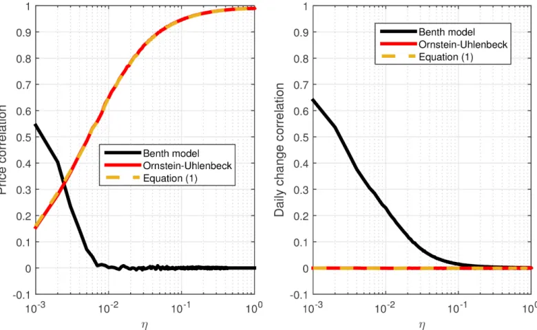
We compared between Eqs (1–3), given the same value ofσ(or standard deviation ofωt).
10000 reference time series,It, of 1000 time steps (or days) were considered for different values
ofη. The reference time series were defined as done in the previous section (I1= 1;
It¼ Qt
j¼21þj, where for eachj,jfollowsNð0;0:0001Þ). We used the 3 models to construct
a time seriesXt. We calculated the correlation betweenXtandItand between the daily relative
change of each of these series. For each value ofηwe considered the average value of these
Fig 2. The dependence of the index-stocks correlation onη.The average correlation betweenItand
arbitrary modeled stock, based on 5000 runs of the model, is presented for several series length (1000, 2000, 3000, 4000 and 5000 days) forηrunning from 0 to 1.
correlations (within the 10000Itseries), so we could compare the results depicted in Figs1and
2between the different models. The results of the comparison are presented inFig 3.
As demonstrated by the results inFig 3, the results forEq (1)and for the standard version of the Ornstein-Uhlenbeck process (for non constantμ) are almost identical. The Benth model is naturally inappropriate for modeling the effect of driving external forces on the price in the way described in the previous section.
It is possible to produce a smoothed time series for eachItusing LOWESS method [37]. The
similarity of the results forItand for the smoothed time series,I~t, is found to be very high (see
S3 Fig) and preserves the fundamental property of high stock-index price correlation and 0
cor-relation in the return. Using a smoothedItis a more realistic assumption than considering the
value itself, since in practice a stock price can significantly diverge from the external force value. However, proper normalization eliminates the need for considering a smoothed approximate time series for the external driving force. In the next sections, thefinancial data analyzed will be normalized so that the average value of the stock price equals that of the index. This normaliza-tion is necessary, as otherwise the expressionðIt 1 X
i
t 1ÞinEq (1)is essentially meaningless.
The shipping market as a test case
Following the model derivation, a statistical characterization of market sectors is essential in order to validate it. We will try to capture the unique statistical properties of stocks that belong
to a certain sector and traded in stock markets. Such stocks can belong not only to the same sector but also to the same market (for example, if traded in the same stock exchange). There-fore, each stock can be characterized according to several categories of belonging, most notably its stock market index and the driving force dominating its sector.
In order to perform this characterization, we first address the shipping sector, which func-tions as a test case for a sector dominated by an external force. By characterizing this sector spe-cifically, we will be able to derive general conclusions regarding the nature of sectors and compare these conclusions with the model results.
The shipping stock market is a unique sector in the financial market, in which stock prices are ultimately regulated by external parameters. Most notably, these parameters include fuel prices, raw material and infrastructure demand as well as various commodity prices [19,38]. Because the international shipping industry facilitates 90% of world trade and is a key factor in global economic development, it is a major factor in economic and financial theory [39–41]. The shipping industry is tightly linked to the world economy and to the international trade business cycle. Therefore, it enjoyed a long prosperous period with growing trade at the inter-national level until the financial crisis in 2008 [41–44]. The shipping industry is also dynamic and volatile. The volatility in shipping markets is significantly higher (0.79%) than the average volatility in commodity markets (0.5%) and equity markets (e.g., S&P500 0.2%) [44]. This extremely high risk is not only due to volatility in global economic cycles, but is also highly influenced by intrinsic characteristics of the shipping industry itself [19]. Naturally, the ship-ping market stocks are linked both to the stock market, represented by the stock market index, and to external driving forces.
TheBaltic Dry Index(BDI) [44] is an index issued daily, which provides an assessment of the price of transporting dry cargo (such as grains, coal, ore and cement) by sea, representing the physical market. Its value is measured in US dollars (though arbitrary, in fact) and deter-mined by a panel of international shipbrokers. As such, important information is contained in its value, substantially affecting the shipping market.
In order to analyze the relationship between the BDI and different shipping market stocks, the correlation between them was calculated. We used 4 different stocks—DSX, DRYS, PRGN and WILS, 4 leading shipping companies focusing on dry bulk market, and calculated the cor-relations for the period 2007–2014. The results are presented inFig 4.
The correlation between the BDI and the price of the shipping companies examined is very high, meaning that indeed, the BDI reflects relatively well the state of the shipping industry. However, there is only a weak positive correlation between the daily change of the BDI and the daily return of the stocks. It should be noted, in addition, that the correlation between these stocks and the BDI is much higher (0.8–0.9) than the positive correlation that exists between stocks and the stock market index (0.2–0.4) [20,45–49]. Therefore, the high correlation found cannot be explained by the overall market behavior, although it affects both the stocks of ship-ping companies and even the BDI, but only weakly. This is also illustrated inFig 5, in which the historical PRGN stock price is presented along with the BDI and the NASDAQ Composite index to which the PRGN stock belongs. The positive correlation between the stock price and the stock market index (0.2) is much lower than the correlation between the stock price and the BDI (0.96). However, when the daily relative change is compared, we obtain a correlation of 0.5 between the daily relative change of the PRGN stock price and the NASDAQ Composite index, and 0.1 between the PRGN stock price and the BDI daily change.
The correlation matrices depicted inFig 4are similar in structure and values to the model results presented inFig 1. The similarity was also tested using aχ2test, considering 5 degrees of
Fig 1serve as a good fit to the real correlation matrices withp<0.01. This demonstrates that
the model can represent the actual financial data regarding the correlation structure in market sectors, particularly in the shipping sector.
In addition, the stock prices analyzed were found as cointegrated with each other, as well as cointegrated with the BDI value (withp<0.01) and all the stocks are found to Granger cause
Fig 4. The correlation structure in the shipping market.The correlation in the price (A) and in the daily change (B) between the Baltic dry index and stocks of 3 shipping companies traded in New York stock exchange (NYSE)—DSX, DRYS and PRGN—and one in Oslo stock exchange—WILS—for the period 2007–2014 (seeS1 Table).
doi:10.1371/journal.pone.0152487.g004
all others and the BDI (and vice versa) withp<0.01. These properties are most probably
origi-nated by the substantial effect of the BDI on the stocks. Their return, however, as implied from
Fig 4, is not cointegrated with the daily changes of the BDI.
Together with the previous results, a clearer picture of the dynamics of the shipping market emerges. On the daily time scale, the BDI is not a strong effector on the shipping market stocks. The daily returns of the stocks are governed by the fluctuative nature of stock market trade, by news flow and by the patterns of the investors’behavior [20,50,51]. However, on a longer time scale, such as the monthly or annual time scales, the trend of the stocks is close to the trend of the BDI, which represents the state of the physical shipping market.
The model results and the analyzed data demonstrate that the model produces results that agree with the statistical properties of the market sectors, as presented for the shipping market. In particular, the modeled stocks present high correlation (as a function ofη) with the value of
the external driving force, while their daily return is independent of the daily change of the force. Consequently, it is observed that a mechanism such as the coupling term in the model can explain the high correlation between the external force and the stock prices on a long time scale, without changing the uncorrelated behavior on shorter time scales.
We note that using a normal distribution for the daily change is not based on real data. The real return distribution approximately follows a Lévy distribution [20]. However, this differ-ence is insignificant in the context of the behavior analyzed (seeS2 Figfor additional informa-tion). The realistic return distribution does not contradict the model results, yet it is simply unnecessary for demonstrating the presented effect of the external forces on stock prices. Therefore, for simplicity, a normal distribution is used.
Following these results it is possible to estimate the value ofηfor specific driving forces and
stocks, and particularly, for the shipping market. The average correlation between the BDI and the analyzed shipping market stocks was 0.89, which approximately corresponds toη= 0.025,
according to the model results. If the BDI is taken asItwe can produce simulated prices of “shipping”stocks. The model was used to create a simulated time series for the PRGN stock, using the appropriate number of days (1772) and the appropriate value ofηcorresponding to
the correlation between the PRGN stock price and the BDI (η= 0.062).Fig 5presents this
calculation.
The results demonstrate that the simulated stock prices highly resemble the original stock price and their average correlation with the BDI is almost identical (0.955) to the correlation of the original stock (0.956). The correlation between the PRGN stock price and the simulated stock prices was 0.97 on average. As expected, the daily return of these two stocks displays an insignificant correlation (0.04). The appropriate value taken forη(0.062 or 6.2%) lies in a
sen-sible domain of values [52,53]. Furthermore, the difference between the various realizations is very small. The modeled stock price time series was also found to Granger cause the BDI time series withp<0.01, as expected.
The results presented so far indicate that the coupling model devised captures the statistical characteristics of market sectors and can be applied for the shipping market. By properly adjusting the value ofη, an artificial stock price time series is created, such that its quantitative
behavior is similar to real stock prices within the shipping market. This confirms the underly-ing assumptions of the model, and the mechanism by which the external drivunderly-ing force effects the sector stock prices.
market the gold price was taken as the external forceIt, and the stock prices of 4 leading gold
mining companies were considered—Goldcorp Inc. (GG), Barrick Gold Corporation (ABX), Silver Wheaton Corporation (SLW) and Franco-Nevada Corporation (FNV). For the food pro-duction market we used the wheat price as the external force, and the stock prices of 4 grains and food manufacturing companies were considered—Archer Daniels Midland Company (ADM), Bunge Limited (BG), Nestlé S.A. (NSRGY) and Ingredion Inc. (INGR). For more details, refer toS1 Table.
The correlations between the different stocks and the external forces were calculated. This calculation was done both between the stock prices and the external force values and between the stock returns and the external force relative daily change time series, as done for the ship-ping market stocks. The results are presented inFig 6.
The correlation between the gold price and the price of the gold mining companies exam-ined, as well as for the wheat price and food companies, is very high (except for ABX). As implied by the results for the shipping market, the results demonstrate that the gold mining
Fig 6. The correlation structure in the gold mining and food production markets.The correlation in the price (A) and in the daily change (B) between the gold price and stocks of 4 leading gold mining companies traded in NYSE and Toronto stock exchange for the period 2007–2014; The correlation in the price (C) and in the daily change (D) between the wheat price and stocks of 4 leading food companies traded in NYSE and over the counter for the period 1983– 2014.
and food production markets can be regarded as examples for sectors with an external driving force (compare with Figs1and4). There is only a very weak positive correlation between the daily change of the external force and the daily return of the stocks, as found for the shipping market. In addition, all the stock prices (apart from FNV in the gold mining sector) within each of the sectors are found to be cointegrated and Granger cause each other (withp<0.01).
The model was applied to the gold mining market as previously done for the PRGN stock taking the SLW stock for the gold mining sector and the BG stock for the food production sec-tor. The results are presented inFig 7, capturing a similar behavior to the behavior depicted in
Fig 5.
Due to the lower correlation between the stock prices and the driving forces in the gold min-ing and food production sectors, when compared to the shippmin-ing sector, the modeled stock prices obtained are reminiscent of the original stock price. This indicates that the prices of these stocks might be driven by additional driving forces, in particular the stock market index. For example, the correlation between the BG stock price to the S&P500 index to which it belongs, is 0.72, which is almost as high as its correlation to the wheat price. Therefore, in prac-tice, in order to provide a proper model for the stock price, an additional coupling parameter is needed to an additional external driving force. This expansion of the model is left for future work. We note, however, that for most of the stocks, the correlation between their price and the stock market index is about 0.2 to 0.4 [20].
Discussion
We described the statistical properties of market sectors with an external driving force. These sectors are most notably characterized by a long time scale dependence on the driving force, meaning that the trend of the force strongly affects the sector stock prices. However, the short term behavior of the stocks is weakly affected by this force. In particular, the daily return of the sector stocks is effectively independent of the daily change of the external force. The daily return is therefore a result of the market behavior [20,50]. In addition, the stock prices are found to be statistically cointegrated and to Granger cause each other as well. These properties were demon-strated by analyzing the shipping sector, the gold mining sector and the food production sector.
This characteristic behavior motivated us to devise a mean reverting model based on the coupling between sector stock prices and a driving force for the sector stock price dynamics. The model was found successful by reproducing all the described properties. By adjusting one free parameter—the coupling intensity between the external force and the stock prices—we were also able to artificially reproduce the actual stock prices, preserving the statistical proper-ties demonstrated. We note, however, that other statistical properproper-ties related to short term characteristics of financial data, such as intraday behaviors, the return distribution and the slow decay of the autocorrelation with the lag, are irrelevant within the scope of this model. At this stage, we only capture the behavior of stock prices within sectors, which are affected by external forces and unaffected by these statistical properties.
The findings of this work, together with the study of short term herd behavior phenomena in the stock market [20], demonstrate that the full description of the dynamics of stocks, can be done by integrating multiple time scales and multiple dominating forces or indices [48]. Nota-bly, we found that along with short time scale coupling between stock prices to the stock market index [18,20,48], there exists a longer time scale coupling to a sector specific external force.
the diversification of risk in the financial market, notably under market stress. Empirical obser-vations demonstrate that in times of stress, correlations within the financial markets increase [54], so that on a long time scale, sectors governed by external driving forces, might reduce the importance of such effects [11–13].
It follows that each stock has several categories of belonging, corresponding most notably with its stock market index and an external driving force dominating its sector. For example, when analyzing the shipping market we considered the stock WILS, which is traded in the Oslo stock exchange. WILS demonstrated a very low correlation between its daily return and the daily return of the other shipping stocks considered, which are traded in the NYSE. How-ever, on a longer time scale, the prices of WILS and the other stocks were highly correlated, due to the effect of the BDI. In addition, the stock index might also have an effect on stock prices on a longer time scale which is smaller than the effect of the BDI or the external driving forces in general. Such an effect might be associated with the discrepancy depicted in Figs5and7
between the modeled stock price and the real stock price. Introducing an additional coupling parameter between the modeled stock price and the stock market index might improve the model accuracy. Following this, a more intricate measure of similarity between the stock price, the index and the external driving force should be introduced, as correlation will be insufficient as such measure in this case.
FollowingEq (1), and by omitting the statistical noise, the parameterηcan be mathematically
interpreted as the reciprocal of a characteristic time scale. For example, taking a time interval of one day,η= 0.01 can be associated with a characteristic time of 100 days. This time characterizes
the process of the stock price convergence into the driving force value. The statistical noise plays an important role and therefore this interpretation is not exact. However, it introduces a charac-teristic time scale to the dynamics described by the model. The values ofηassociated with the
sectors presented previously, stand for characteristic time scales ranging approximately from 25 to 200 days, and confirm the notion of long term effect of the external driving forces.
More research should be carried out to establish the above: The integration of the model with the herd behavior model for the shorter time scale [20] to provide a model consistent with mar-ket phenomena on a variety of time scales; expansion of the model to include an approximate
Fig 7. Simulated gold mining and food production stock prices.(Left) The gold price is displayed (blue) along with the real SLW stock price (red) and the averaged price of 1000 model realizations usingη= 0.02 (green); (Right) The wheat price is displayed (blue) along with the real BG stock price (red) and the averaged price of 1000 model realizations usingη= 0.006 (green). The error bars signify±1σ.
smoothed time series for the external force to provide a more realistic driving effect on the stock prices; expansion of the model to include additional important statistical attributes of the driving forces; further validation of the model by considering additional economies and sectors; consid-ering additional measures of similarity between stock prices and driving forces; relating the results to risk assessment, specifically in times of financial stress or crisis.
Supporting Information
S1 Fig. The model results with and without stock-stock return correlation.A randomwalk
was used asIt(thick blue curve), and following the presented coupling model, the prices of 4
stocks were constructed and presented for 1000 days and forη= 0.05. It was taken without any
correlation between the daily returns of the different stocks (A) and given the actual correla-tions for the shipping stocks analyzed (seeFig 4in the paper) (B). In addition, the correlation structure is presented—the correlation matrices of the price without (C) and with daily return correlation (D), as well as for the daily return without (E) and with daily return correlation (F). (EPS)
S2 Fig. Comparison between normal and Lévy distributed returns.(A) The dependence of
the index-stocks correlation onηfor normal distributed returns (blue) and Lévy distributed
returns (green); Also presented are the correlation matrices of the price forη= 0.01 (B) and the
return (C) for the Lévy distributed returns. Compare these results toFig 1in the paper. The parameters used for the Lévy distributed return were taken from the analysis of the Baltic dry index daily change (for the external force) and from typical values for the daily return of stock traded in the stock market (for the stocks).
(EPS)
S3 Fig. The dependence of the index-stocks price and return correlation onηfor different
models.(A) One realization ofItandI~ttime series, smoothed using the LOWESS method; (B)
The dependence of the index-stocks correlation onηfor the Benth model (black), the
Orn-stein-Uhlenbeck process (red),Eq (1)model (dashed yellow curve) and forEq (1)model calcu-lated using~It(green); (C) The dependence of the index-stocks return correlation onηfor the
Benth model (black), the Ornstein-Uhlenbeck process (red),Eq (1)model (dashed yellow curve) and forEq (1)model calculated using~It(green).
(EPS)
S1 Table. Summary of all data sets used in the empirical analysis for the model validation. In order to validate the model, we use empirical data and compare to model results to the char-acteristics of different sectors in the market. The data used is for the dry shipping market, the gold mining sector and the food production sector and based on various databases [55–57]. The following table summarizes all the data sets used in this analysis and their sources. (PDF)
Acknowledgments
This research has been supported in part by the Tauber Family Foundation and the Maguy-Glass Chair in Physics of Complex System at the Tel-Aviv University.
Author Contributions
References
1. Gindling TH (1991). Labor market segmentation and the determination of wages in the public, private-formal, and informal sectors in San Jose, Costa Rica. Econ Devel Cult Change. 1991; 39: 585–605. doi:10.1086/451892
2. Cooke TE. The impact of size, stock market listing and industry type on disclosure in the annual reports of Japanese listed corporations. Account Bus Res. 1992; 22: 229–237. doi:10.1080/00014788.1992. 9729440
3. Campbell JY, Lo AWC, MacKinlay AC. The econometrics of financial markets ( Vol. 2). Princeton: Princeton university press; 1997.
4. Mantegna RN. Hierarchical structure in financial markets. Eur Phys J B. 1999; 11: 193–197. doi:10. 1007/s100510050929
5. Wurgler J. Financial markets and the allocation of capital. J Financ Econ. 2000; 58: 187–214. doi:10. 1016/S0304-405X(00)00070-2
6. Beck T, Demirgüç-Kunt A, Levine R. A new database on the structure and development of the financial sector. World Bank Econ Rev. 2000; 14: 597–605. doi:10.1093/wber/14.3.597
7. De Bandt O, Davis EP. Competition, contestability and market structure in European banking sectors on the eve of EMU. J Bank Financ. 2000; 24: 1045–1066. doi:10.1016/S0378-4266(99)00117-X
8. Bourlès R, Cette G, Lopez J, Mairesse J, Nicoletti G. Do product market regulations in upstream sectors curb productivity growth? Panel data evidence for OECD countries. Rev Econ Stat. 2000; 95: 1750– 1768.
9. Gopikrishnan P, Rosenow B, Plerou V, Stanley HE. Quantifying and interpreting collective behavior in financial markets. Phys Rev E. 2001; 64: 035106. doi:10.1103/PhysRevE.64.035106
10. Uechi L, Akutsu T, Stanley HE, Marcus AJ, Kenett DY. Sector dominance ratio analysis of financial markets. Physica A. 2015; 421: 488–509. doi:10.1016/j.physa.2014.11.055
11. Ellis F. Household strategies and rural livelihood diversification. J Dev Stud. 1998; 35: 1–38. doi:10. 1080/00220389808422553
12. Imbs J, Wacziarg R. Stages of diversification. Am Econ Rev. 2003; 93: 63–86. doi:10.1257/ 000282803321455160
13. Iacobucci D, Rosa P. Growth, diversification, and business group formation in entrepreneurial firms. Small Bus Econ. 2005; 25: 65–82. doi:10.1007/s11187-005-4258-8
14. Kinlaw W, Kritzman M, Turkington D. Toward determining systemic importance. J Portfolio Mgt. 2012; 38: 100–111.
15. Granger CWJ. Investigating causal relations by econometric models and cross-spectral methods. Econometrica. 1969; 37: 424–438. doi:10.2307/1912791
16. Granger CWJ, Newbold P. Spurious regressions in econometrics. J Econometrics. 1974; 2: 111–120. doi:10.1016/0304-4076(74)90034-7
17. Borghesi C, Marsili M, MiccichèS. Emergence of time-horizon invariant correlation structure in financial returns by subtraction of the market mode. Phys Rev E. 2007; 76: 026104. doi:10.1103/PhysRevE.76. 026104
18. Kenett DY, Tumminello A, Madi A, Gur-Gershgoren G, Mantegna RN, Ben-Jacob E. Dominating clasp of the financial sector revealed by partial correlation analysis of the stock market. PLOS ONE. 2010; 5: e15032. doi:10.1371/journal.pone.0015032PMID:21188140
19. Zhang X, Podobnik B, Kenett DY, Stanley HE. Systemic risk and causality dynamics of the world inter-national shipping market. Physica A. 2014; 415: 43–53.
20. Shapira Y, Berman Y, Ben-Jacob E. Modelling the short term herding behaviour of stock markets. New J Phys. 2014; 16: 053040. doi:10.1088/1367-2630/16/5/053040
21. Berman Y, Shapira Y, Ben-Jacob E. Unraveling Hidden Order in the Dynamics of Developed and Emerging Markets. PLOS ONE. 2014; 9: e112427. doi:10.1371/journal.pone.0112427PMID:
25383630
22. Sandoval L Junior, Mullokandov A, Kenett DY. Dependency relations among international stock market indices. J. Risk Financial Manag. 2015; 8: 227–265. doi:10.3390/jrfm8020227
23. Engle RF, Granger CWJ. Co-integration and error correction: representation, estimation, and testing. Econometrica. 1987; 55: 251–276. doi:10.2307/1913236
24. Mantegna RN, Stanley HE. Econophysics: Scaling and its breakdown in finance. J Stat Phys. 1997; 89: 469–479. doi:10.1007/BF02770777
26. MiccichèS, Bonanno G, Lillo F, Mantegna RN. Degree stability of a minimum spanning tree of price return and volatility. Physica A. 2003; 324: 66–73. doi:10.1016/S0378-4371(03)00002-5
27. Sharpe WF. Capital asset prices: A theory of market equilibrium under conditions of risk. J. Finance. 1964; 19: 425–442. doi:10.2307/2977928
28. Cox JC, Ingersoll JE Jr., Ross SA. An intertemporal general equilibrium model of asset prices. Econo-metrica. 1985; 53: 363–384. doi:10.2307/1911241
29. Black F, Derman E, Toy W. A one-factor model of interest rates and its application to treasury bond options. Financ Anal J. 1990; 46: 33–39. doi:10.2469/faj.v46.n1.33
30. Uhlenbeck GE, Ornstein LS. On the theory of the Brownian motion. Phys Rev. 1930; 36: 823–841. doi:
10.1103/PhysRev.36.823
31. Poterba JM, Summers LH. Mean reversion in stock prices: Evidence and implications. J Financ Econ. 1988; 22: 27–59. doi:10.1016/0304-405X(88)90021-9
32. Cecchetti SG, Lam PS, Mark NC. Mean reversion in equilibrium asset prices. NBER Working Paper No. w2762. 1988.
33. Benth FE, Benth JÅ. The volatility of temperature and pricing of weather derivatives. Quant Finance. 2007; 7: 553–561. doi:10.1080/14697680601155334
34. Zapranis A, Alexandridis A. Modelling the Temperature Time-dependent Speed of Mean Reversion in the Context of Weather Derivatives Pricing. Appl Math Finance. 2008; 15: 355–386. doi:10.1080/ 13504860802006065
35. Benth FE, Benth JÅ, Koekebakker S. Stochastic modelling of electricity and related markets ( Vol. 11). Singapore: World Scientific; 2008.
36. Wong HY, Lo YW. Option pricing with mean reversion and stochastic volatility. Eur J Oper Res. 2009; 197: 179–187. doi:10.1016/j.ejor.2008.05.014
37. Cleveland WS. LOWESS: A Program for Smoothing Scatterplots by Robust Locally Weighted Regres-sion. Am Stat. 1981; 35: 54–54. doi:10.2307/2683591
38. Zhang X, Shao S, Stanley HE, Havlin S. Dynamic motifs in socio-economic networks. Europhys Lett. 2014; 108: 58001. doi:10.1209/0295-5075/108/58001
39. Grammenos CT, Arkoulis AG. Macroeconomic factors and international shipping stock returns. Int J Marit Econ. 2002; 4: 81–99. doi:10.1057/palgrave.ijme.9100033
40. Samitas AG, Kenourgios DF. Impact of mergers and acquisitions on stock returns of tramp shipping firms. J Financ Serv Manag. 2007; 2: 327–343.
41. Branch A, Stopford M. Maritime Economics. New York: Routledge; 2013.
42. Krafft M. International Shipping in Crisis: Background, Framework and Implications. EU: GRNI Press; 2010.
43. Albertijn S, Bessler W, Drobetz W. Financing Shipping Companies and Shipping Operations: A Risk-Management Perspective. J Appl Corp Financ. 2011; 23: 70–82. doi:10.1111/j.1745-6622.2011. 00353.x
44. Drobetz W, Richter T, Wambach M. Dynamics of time-varying volatility in the dry bulk and tanker freight markets. Appl Financ Econ. 2012; 22: 1367–1384. doi:10.1080/09603107.2012.657349
45. Allez R, Bouchaud JP. Individual and collective stock dynamics: intra-day seasonalities. New J Phys. 2011; 13: 025010. doi:10.1088/1367-2630/13/2/025010
46. Goswami B, Ambika G, Marwan N, Kurths J. On interrelations of recurrences and connectivity trends between stock indices. Physica A. 2012; 391: 4364–4376. doi:10.1016/j.physa.2012.04.018
47. Song DM, Tumminello M, Zhou WX, Mantegna RN. Evolution of worldwide stock markets, correlation structure, and correlation-based graphs. Phys Rev E. 2011; 84: 026108. doi:10.1103/PhysRevE.84. 026108
48. Shapira Y, Kenett DY, Ben-Jacob E. The index cohesive effect on stock market correlations. Eur Phys J B. 2009; 72: 657–669. doi:10.1140/epjb/e2009-00384-y
49. Kenett DY, Shapira Y, Madi A, Bransburg-Zabary S, Gur-Gershgoren G, Ben-Jacob E. Index cohesive force analysis reveals that the US market became prone to systemic collapses since 2002. PLOS ONE. 2011; 6: e19378. doi:10.1371/journal.pone.0019378PMID:21556323
50. Preis T, Moat HS, Stanely HE. Quantifying trading behavior in financial markets using Google Trends. Sci Rep. 2013; 3: 1684. doi:10.1038/srep01684
51. Moat HS, Curme C, Avakian A, Kenett DY, Stanely HE, Preis T. Quantifying Wikipedia usage patterns before stock market moves. Sci Rep. 2013; 3: 1801. doi:10.1038/srep01801
53. Podobnik B, Fu DF, Stanley HE, Ivanov PC. Power-law autocorrelated stochastic processes with long-range cross-correlations. Eur Phys J B. 2007; 56: 47–52. doi:10.1140/epjb/e2007-00089-3
54. Preis T, Kenett DY, Stanley HE, Helbing D, Ben-Jacob E. Quantifying the behavior of stock correlations under market stress. Sci Rep. 2012; 2: 752. doi:10.1038/srep00752PMID:23082242
55. Clarkson’s Shipping Intelligence Network database. 2014. Accessed:http://sin.clarksons.net. 56. Yahoo! Finance database. 2014. Accessed:http://finance.yahoo.com.