The causal effect of family size on child labor and education

(1)

T

HE

C

AUSAL

E

FFECT OF

F

AMILY

S

IZE ON

C

HILD

L

ABOR AND

E

DUCATION

VLADIMIR PONCZEK AND ANDRE PORTELA SOUZA

Julho

de 2007

T

e

x

t

o

s

p

a

r

a

D

(2)

TEXTO PARA DISCUSSÃO 162 • JULHO DE 2007 • 1

The Causal Effect of Family Size on Child Labor and

Education

Vladimir Ponczekand Andre Portela Souza

R

ESUMO

P

ALAVRAS CHAVES

C

LASSIFICAÇÃO

JEL

J13,I21

A

BSTRACT

This paper investigates the causal relationship between family size and child labor and education among Brazilian children. More especifically, it analyzes the impact of family size on child labor, school attendance, literacy and school progression. It explores the exogenous variation in family size driven by the presence of twins in the family. The results are consistent under the reasonable assumption that the instrument is a random event. Using the nationally representative Brazilian household survey (PNAD), detrimental effects are found on child labor for boys. Moreover, significant effects are obtained for school progression for girls caused by the exogenous presence of the young siblings in the household.

K

EY

W

ORDS

(3)

TEXTO PARA DISCUSSÃO 162 • JULHO DE 2007 • 2

Os artigos dos Textos para Discussão da Escola de Economia de São Paulo da Fundação Getulio Vargas são de inteira responsabilidade dos autores e não refletem necessariamente a opinião da

FGV-EESP. É permitida a reprodução total ou parcial dos artigos, desde que creditada a fonte.

Escola de Economia de São Paulo da Fundação Getulio Vargas FGV-EESP

(4)

The Causal Effect of Family Size on Child Labor and Education

Vladimir Ponczek∗_{and Andre Portela Souza}†

June 14, 2007

Preliminary draft. Please do not quote without permission. Comments welcome.

Abstract

This paper investigates the causal relationship between family size and child labor and

education among Brazilian children. More especifically, it analyzes the impact of family size

on child labor, school attendance, literacy and school progression. It explores the exogenous

variation in family size driven by the presence of twins in the family. The results are consistent

under the reasonable assumption that the instrument is a random event. Using the nationally

representative Brazilian household survey (PNAD), detrimental effects are found on child labor

for boys. Moreover, significant effects are obtained for school progression for girls caused by the

exogenous presence of the young siblings in the household.

(5)

1 Introduction

The economic literature has discussed the relationship between family size and child quality for

quite some time. It has been argued that there is a trade-off between quantity and quality of

children (Becker and Lewis (1973), Becker and Tomes (1976), and Hanushek (1992)). In general,

child quality is understood as any child outcome that is valued by the parents. In practice, authors

have in mind the wellbeing of the child or her accumulation of human capital. Becker and Lewis

(1973) developed a model which introduces a theoretical framework to analyze this issue. They

assume that the cost of an additional child (holding quality constant) is greater as the number

of children increases. Similarly, the cost of increasing the average quality of a child rises (holding

quantity constant) as quality increases. An important implication of such models is that family

size becomes an input in the production of child quality.

In principle, the impact of family size on child quality can be harmful or beneficial. One

can imagine a situation where the larger the family is, the more the resources are diluted. For

instance, in an environment where credit markets are imperfect, families with many children would

invest less in each child than if they have fewer children. However, it is possible that having more

children decreases maternal labor supply (Angrist and Evans (1998)). Thus, as argued by Blau and

Grossberg (1992) this reduction could increase the probability that the mother spends more time

parenting which could improve the child quality.

Child labor is a common phenomenon in developing countries. It is often used by the families to

complement their total resources (see Basu (1999), Edmonds and Pavcnik (2005), and Edmonds and

Pavcnik (2006) for surveys on child labor). Child labor is typically associated with lower human

capital formation (Beegle et al. (2006), Emerson and Souza (2006)). The theoretical literature

emphasizes the trade-off between child labor and human capital accumulation. The main channels

are time constraints (the child has less time to acquire education) as well as the physical and

psychological constraints (the child is less capable of learning after hours of work) (e.g. Baland

(6)

child quality as long as human capital formation is an attribute valued by the parents. However,

some economists argue that child labor can be a resource to finance the child education (e.g.

Psacharopoulos (1997)). In this case, an extra child would raise the family income required to

invest in child quality.

Measuring the impact of family size on child quality outcomes is an empirical endeavor. An

important feature to be taken into account is that child quality and quantity are jointly determined

by the parents. For instance, in the Becker and Tomes (1976) model, families decide how many

children to have and how much to invest in each child. Given the nonlinear constraints, an exogenous

increase in the number of children raises the per child cost of quality. Thus, the model implies that

there is a negative causal relation between quantity and quality.

However, a negative association between quality and quantity could be driven by other factors.

For example, parents’ endowment (such as ability, wealth, education, and cultural factors) affects

the child quality by intergenerational transmission mechanisms. Low-endowed parents may produce

low-endowed children who benefit less from an extra investment in their quality compared to

high-endowed children. If this is the case, parents with low endowments would optimally decide to have

more children and lower quality per child compared to high-endowed parents. Again, one would

observe a negative correlation between quantity and quality but now not driven by an exogenous

change in the family size. Therefore, this correlation would not be causal.

By the same token, child labor and fertility are ambiguously related. It is possible to show in

the Baland and Robinson (2000) model when fertility is exogenous that an increase in family size

decreases the amount worked by each child. This occurs because having more children may increase

the total family income reducing the required labor intensity per child. However, if fertility and

child labor are jointly determined, the direction of causality is not clear. On one hand, increasing

child labor reduces the net cost of a child, raising the demand for children. On the other hand,

increasing fertility increases the total cost of all children and requires more child labor to generate

the extra income. Additionally, Cigno and Rosati (2005) illustrate a model where wealth and

(7)

fertility and child labor and education would be driven by a third factor. The causal effect of the

former on the latter would not be necessarily present.

Any empirical exercise which tries to estimate the causal effect of family size on child quality

must take into consideration the endogeneity of fertility. The empirical literature concerned with

industrialized countries that deals with this endogeneity problem focuses on educational outcomes.

The results are mixed. Black et al.(2005) find no impact of family size on children’s educational

attainment in Norway. Haan (2005) finds no significant effect of thenumber of children on

educa-tional attainment in US and Netherlands. Angrist et al. (2005) and Angrist et al. (2006) do not

find any causal impact of family size on completed educational attainment and earnings in Israel.

Conley and Glauber (2005) using the 1990 US PUMS estimate that children living in larger families

are more likely not to attend private school and be held back in school. And Goux and Maurin

(2005) show that children living in larger families perform worse in school than children in smaller

families in France. They claim that the mechanism is due to overcrowded homes. For developing

countries, using data from India between 1969 and 1971, Rosenzweig and Wolpin (1980) estimate

that households with higher fertility had lower levels children’s schooling. Lee (2004) finds negative

impacts of family size on per child investment in education for South Korean households.

To the best of our knowledge, the literature lacks studies on the determinants of child labor

that correctly take into account the endogeneity of family size. For instance, Psacharopoulos and

Patrinos (1997) find that having more young siblings is associated with less schooling, more

age-grade distortion, and less child labor among Peruvian children in 1991. Cigno and Rosati (2002)

studying the determinants of child labor and education in rural India find a significantly positive

effect of the number of children aged 6-16 on the time used to work and a negative effect on

the time used to attend school. Although these works are an important step for understanding

the determinants of child labor, the potential endogeneity of fertility can bias their results and

mislead the conclusion they found. The only attempt made to deal with endogeneity problem of

the relationship between child labor and fertility is in Deb and Rosati (2004). They use the gender

(8)

for fertility. They find a positive effect ofnumber of children on the probability of work when the

endogeneity is taken into account. This result is different from the case when fertility is assumed to

be exogenous. In this case, they find an insignificantly negative effect on child labor. Although their

study is a valid attempt to deal with the endogeneity of fertility, we doubt that the instruments

have the indispensable characteristic of being orthogonal to the unobservables. It is very likely

that the instruments, especially the parents’ ages and the village mortality rate, are correlated to

wealth, ability and others unobservable variables that could be jointly related with child labor and

fertility, jeopardizing their results and conclusions.

The objective of this paper is to gauge the causal effect of family size on child labor and

educational outcomes in a developing country context. More specifically, we obtain the impact of

family size on child labor, school attendance, literacy rate, and school progression among Brazilian

children. In order to consistently estimate these causal effects we make use of instrumental variable

technique. We explore the exogenous variation of family size driven by the presence of twins in

the family. We believe that our results are consistent under the reasonable assumption that this

instrument is a random event. We use the nationally representative household surveys (PNAD) for

2001 to 2004. We find that this exogenous increase in family size has different effects on outcomes for

boys and girls. For boys, increase in sibship size are positively related to child labor and negatively

related to school progression. For girls, we only find significant effects on school progression caused

by the exogenous presence of young siblings in the household. Moreover, we examine whether these

impacts marginally differ with family size. The results suggest that the greatest impact lies on the

exogenous change from one to two children.

Correctly estimating the causal effect of family size on child quality outcomes is important for

a developing country public policy perspective. It is well known that the majority of larger families

are poorer and our results suggest that the size of the family has a direct impact on important

social outcomes for children. This discussion can better inform the public debate about how to

understand and address poverty, education, and child labor in developing countries.

(9)

The identification strategy is presented in section 3. The results are discussed in section 4. Section

5 concludes.

2 Data

The data used here come from thePesquisa Nacional por Amostra de Domic´ılios(PNAD) database.

The PNAD is an annual household survey, with sample size equal to 1/500 of the Brazilian

pop-ulation (about 100,000 households) and is designed to produce a picture of the social-economic

conditions of the Brazilian population. It covers all urban and almost all rural areas, except the

Amazon region. It has been conducted in regular basis since 1981 by IBGE (Brazilian Census

Bureau) except in years in which census data were collected (1991 and 2000) and a year with

budget constraint (1994). PNAD also contains extensive information on personal and household

characteristics. For each person, information about age, schooling attendance, literacy, years of

completed schooling, migration, labor participation, retirement, income sources (including values),

etc. is available. We used the 2001, 2002, 2003 and 2004 PNAD’s. We pooled these four surveys

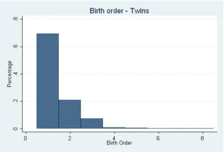
in order to obtain sufficient number of observations for our instrument, since the birth of twins is

a rare event.

Our entire sample consists of children between seven and fifteen years old. Seven years old is the

mandatory school entry age in Brazil1

. We restrict the children’s age to be at most fifteen, since at

fifteen the individual is expected to have completed the middle school cycle (ensino fundamental)

and above this age they are more likely to live outside their parent’s household and are allowed to

work by the Brazilian law. For analyzing child labor, we only include children between ten and

fifteen since PNAD does not have the information about labor participation for children younger

than ten.

PNAD allows us to identify who the mother of each child in the family is, as long as the mother

lives in the same household. Therefore, in order to identify the twins we use year and month

1

(10)

of birth for children with the same mother2

. We exclude from the sample all families in which

the mother was dead or not present. We also excluded families with triplets, quadruplets, and

quintuplets. To identify the twins and number of siblings we use all children younger than sixteen.

Our instrumental variable for the number of children is the presence of twins in the family.

Additionally, the sample is restricted to only include families with two adults (the mother and

her husband) to avoid dealing with the potential endogenous decision about the number of adults

living together in the same family. Therefore, we are just looking at families composed of two

adults and their children aged between zero and fifteen3

. Thus, the variation of the family size will

come from the number of children between zero and fifteen years old in the family.4

In order to check possible channels through which family size impacts child quality, a

sub-sample is created additionally. Now, we narrow our sub-sample only to families with children ten years

or older and estimate the impact of the number of younger siblings (six years old or less) on them

and investigate if the channel through which family size impacts child quality operates from the

younger to the older siblings.

Note that our sample includes some children that were born after the birth of twins in the

family. One possible critique of this sample selection is that the presence of twins in families that

have children after the birth of twins is not correlated with family size. The family could have stuck

with the previously chosen number of children. For those families, the number of siblings would

still be endogenous.

In an attempt to overcome this potential problem, we create three more sub-samples for

ro-bustness checks. First, we exclude from our original sample families that the twins are not last

born and all families with a single child. In other words, this sub-sample encompasses families with

two or more children and no twins or families with last-born twins. In this sub-sample, we also

2

We did not use day of birth to avoid loosing observation of those twins who were born before and after midnight. Nevertheless, we found just four cases like this in our sample

3

Restricting to two-parent families could lead to a selection bias problem. However, we do not believe that this is a serious problem to our analysis, since of all families with children aged fifteen or less only 16% are not two-parent families

4

(11)

exclude the twins themselves. Moreover, in order to analyze whether the marginal effects ofnumber

of children differ along the family size distribution, we create, secondly, a sub-sample of families

with a single child or first-birth twins; and thirdly, we restrict to three-children families where the

oldest child in families with two non-twins is compared to the oldest child in families in which the

non-twin first-born is followed by second-born twins.

For the sake of completeness, we compare our findings using the presence of twins as instruments

with the results obtained using another instrument also commonly present in the literature, the

sibling-sex composition, that is, the occurrence of the first and second born siblings being of the

same gender. We construct a sample including only first-borns of families with two or more children

and instrument the family size by the variable that indicates if the gender of the first two children

is the same.

A final caveat should be added. The number of children calculated is the number of observed

children living in the household in the week of reference. It is possible that there are more siblings

living outside the households. Thus, these figures might be underestimated. We believe that this

problem is attenuated because we only use two-adult families with children aged at most fifteen.

Children older than eighteen is more likely to live outside and families with young children are

less likely to have eighteen-year-old or more children. Therefore, we think this problem is minor.

Nevertheless, this measurement error is attenuated by the IV approach if the presence of twins is

uncorrelated with the measurement error.

3 Empirical Strategy

The main problem regarding estimating the impact of family size on social-economic indicators is

the potential endogeneity of fertility. The decision about how many children a couple will have and

how much to spend in quality outcomes is likely jointly determined. Both could be correlated with

unobserved variables. It is possible that unobserved endowment characteristic such as ability, and

(12)

Having Cigno and Rosati (2005), Baland and Robinson (2000) and Becker and Tomes (1976) models

as a guide, one can conjecture the possible channels that fertility would be endogenous in regressions

involving child labor and quality outcomes in general. For instance, it is known that some culture

traditions are associated with having bigger families than others, and if families with different

traditions also have unequal perception of the value of education, a simple OLS estimator relating

family size and educational outcomes will be biased. By the same token, wealth and ability are

determinants of affording and the correctly understanding of the use of anticonceptional methods.

If they are also correlated with the children educational and labor outcomes, the OLS will not

capture the causal impact of family size on those quality indicators. Depending on the correlation

between unobservables and family size and also with the dependent variables, the OLS estimator

could be upward or downward biased. If the example above about the relationship between ability

and value of education perception and anticonceptional measures is true, we would expect that a

naive approach would overestimate the actual impact of family size on education. On the other

hand, one can imagine that the parent’s decision of having another child is made after a positive

income shock or expectation of increase in future resources, which could offset part of the extra

burden. In this case, the OLS estimator would underestimate the effect of having the extra child

in the family.

Thus, we need a source of variation of family size orthogonal to any unobserved characteristic

of the households that is also related with the dependent variables. The IV approach will be able

to generate a consistent estimator as long as the excluded instrument is uncorrelated with the

unobserved characteristics but also has an important role in the explanation of the endogenous

variable.

The presence of twins in a family has the two desired characteristics for being a good IV. It is

clearly correlated with the family size and, since it is very likely to be a random occurrence, tends

to be orthogonal to the error term in the main regression. A potential flaw of our strategy rises if

there is any independent effect of the presence of twins on quality that does not operate through

(13)

which may affect the raising of the other children in the family. If that is the case, the impact of

family size on quality would be overestimated.

Our benchmark strategy consists in a 2SLS regression, where, in the first step, we regressnumber

of children (Nij) on the presence of twins (P T) and other predetermined variables (W):

Nj =α+βP Tj+γ′Wij+ǫij (1)

The second step follows5

:

Yij =α+βNˆj+γ′Wij +υij (2)

where Yij is the outcome of interest of children i living with family j, i.e., school attendance,

literacy, school progression - defined as (years of schooling)/(age−6) - and participation in the

work force. W is a vector of control variables such as: age; squared age; gender; family head’s

years of schooling and gender; mother’s age; dummies indicating if the child is white, lives in a

urban and metropolitan area, is a twin herself; and year dummies capturing any ongoing trend on

the dependent variables. We also check if there are different impacts on boys and girls by running

separate regressions for each gender.

Additionally, we investigate whether the presence of an extra sibling younger than 7 years old

has similar effects on quality of older children (ten and above) compared to the presence of an extra

sibling regardless of age6

. We replace the presence of any pair of twins as the IV by the presence

of twins younger than seven.

In order to avoid possible endogeneity brought by families that have children after the birth of

twins, we narrow our sample only to families with twins that have not had any children after the

birth of twins. In other words, we check the impact of the number of siblings on those who were

born before the random event.

5

When calculating the variance and covariance matrices ofǫandυwe allow for correlation of residuals within the family unit.

6

(14)

Furthermore, in order to examine if the impact of the increase in the family size is uniform

along family size, we measure two different local average treatment effects (LATE), gauging the

impacts of having one extra or a third sibling on the oldest child. Two sub-samples are created:

one composed of families with only one pair of twins (Treatment) or singletons (Control) - LATE

1; and a second with a twin oldest child with a pair of twins’ siblings (Treatment) or two

non-twins’ siblings -LATE 2. The coefficient of family size inLATE 1 regression measures compare the

quality outcomes among first-born twins against a singleton. On the other hand,LATE 2 compares

the impacts on first-born quality in families with two children against first-borns in families with

three children where the twins are second birth. These comparisons are obtained by running OLS

regressions.

Following the literature (Angrist and Evans (1998), Conley (2000) and Conley and Glauber

(2005)), we extend our analysis by using the presence of same sex of the first and second children

as instrument. As argued by Blacket al.(2005), it is questionable whether sex composition affects

child quality only through family size. Nevertheless, we present the results comparing families

with two children against three children, using the sex composition of the first and second born as

instrument.

4 Results

Endogeneity is the main concern of any study trying to estimate the causal effect of family size on

socio-economic outcomes. Thus, one must be sure that the variation of the explanatory variable

comes from an exogenous source. Our approach consists in using the presence of twins in the

family as an instrument for family size. Although, the birth of twins seems to be a random event,

some important endogeneity issues must be addressed. Has the surge in fertility treatments (In

Vitro Fertilization Pre-Embryo Transfer - IVF) jeopardized the randomness of a twin’s birth?7

IVF

7

(15)

treatments became available in the mid 80’s, 8

but only popularized in Brazil after the mid 90’s

(Borlot and Trindade (2004)). A relative increase in the age of twin’s mothers would suggest an

influence of IVF on the instrument, since, in general, older women are the majority of the ones

searching for fertility treatments. We found no evidence about that in the data. The evolution

of two variables are displayed in figure 1: the ratio of the mother’s age at birth and the ratio of

the proportion of mothers older than thirty-five at birth (mothers of twins/ mothers of non-twins).

The first thing to be noticed is that mothers of twins are on average older than others. However,

there is no evidence that this ratio has increased after IVF treatment became popular in Brazil.

The same can be said about the proportion of mothers older than thirty-five. The fluctuation is

due to the small number of mothers of twins in this age group in our sample (around twenty five

each year). Nevertheless it does not seem to have a clear positive trend or break in the series after

the mid 90’s. This evidence suggests that the relation between IVF treatments and birth of twins

does not invalidate our instrument.

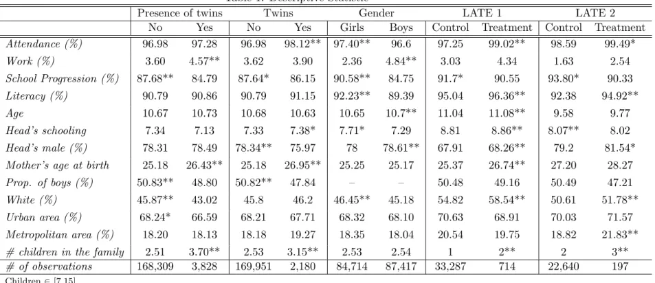
Table 1 shows the main characteristics of the children in the sample. Five different pairs of

groups are compared: children in families with twins (including themselves) against children in

families without twins; twins against non-twins; girls against boys; singletons against a pair of

first-born twins; and the first child in the family with a non-twin sibling against the first child

in the family (non-twin) with two second-born twins. Those who live with twins are significantly

more likely to work and are behind in school progression. The same occurs with twins against

non-twins, but the difference is only statistically significant in the case of school progression. Neither

attendance nor literacy seems to be related with the presence of twins in the family. These results

are not surprising, since Brazil has rapidly increased the school attendance rate after a massive

governmental effort to enroll all children in school reaching 95% of the children between seven and

fifteen years old in 2000 (Souza and Fernandes (2006)). Consequently, the same occurred with

literacy which attained slightly lower indices (89% in 2000). Surprisingly, twins themselves are

significantly more likely to attend school. Families with twins are significantly larger than the

8

(16)

others. The average number of children in family with the presence of twins is 3.70, while this

average is 2.51 children (32.2% smaller) in the other families.

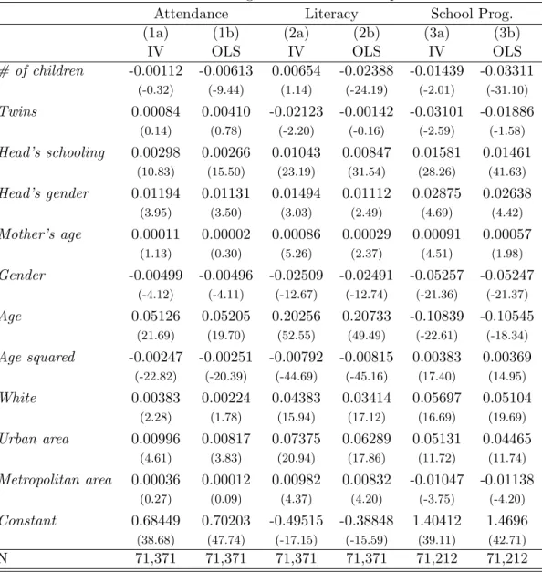
Columns 1b,2b,3b and 4b in table 3 have the OLS regressions for attendance, literacy, school

progression and child labor, respectively. All of them show a strongly significant coefficient of

family size, indicating that children in bigger families are less likely to go to school, to be literate,

are more behind in the school grade and are more likely to work. In general, these figures suggest

a strong detrimental effect of family size in the child quality outcomes.

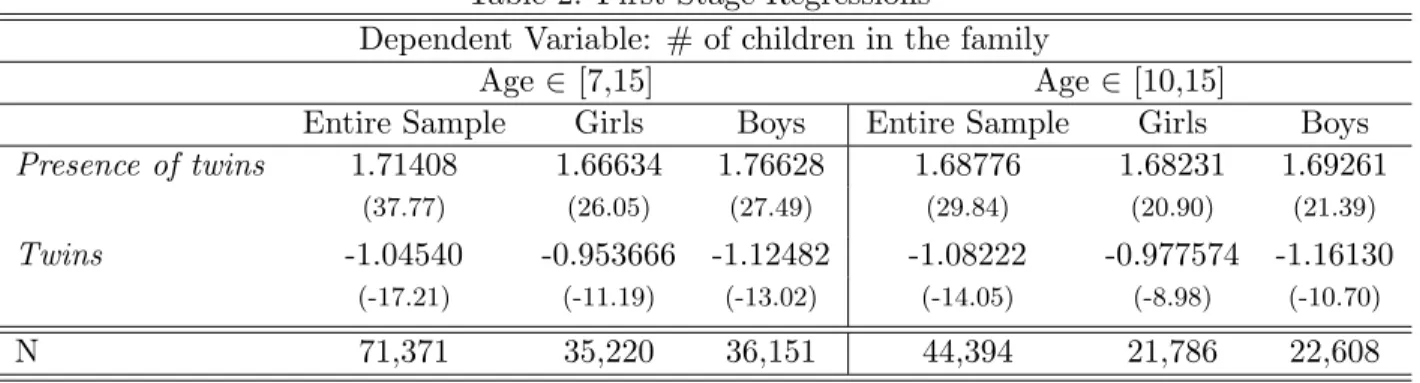
Are those results reliable? First of all, we check if our IV has a strong correlation with the

potential endogenous variable. Table 2 displays the first stage of the IV regressions. The results

corroborate the figures shown in table 1, the coefficient of presence of twins on family size is positive

and significant for the entire sample and also for boys and girls (for both age groups: seven to fifteen

and ten to fifteen years old). The IV regressions displayed in columns1ato4ashow that the impact

of family size is significant and harmful for the children at least for school progression and child

labor. One extra child in the family increases, on average, 1.9% the likelihood of child labor and

increases by 1.4% the school delay. The same cannot be said about school attendance and literacy.

We are unable to reject that the IV results are significantly different from zero. Comparing the

IV with the OLS regressions, we see that for all outcomes but child labor, the OLS bias seems to

overestimate the actual impact of family size. In the case of school progression, the OLS coefficient

is more than two times bigger than the IV one. However, for child labor, using the Wu-Hausman

test, we cannot reject that the OLS estimator is significantly different from the IV one.

Table 4 compares the results for the IV regressions for samples only with girls (columns a)

or boys (columns b). The coefficients of family size are not significantly different from zero for

any of the quality outcomes in the sample only with girls9

. On the other hand, for child labor,

family size is significantly detrimental for boys and we are able to reject that the IV results are

statistically equal to the OLS. Looking at the baseline differences between girls and boys in table

1, we observe that girls on average have higher attendance, literacy, school progression levels and

9

(17)

work less often.10

A possible explanation for these results is that an exogenous change in family

size has a direct impact on the resource available per child. Previous studies have shown that boys

seem to be more affected when there are sudden changes in the family budget constraints, while

girls are somehow “immune” to those variations. Preferences revealed by intra-household allocation

decisions could be the key factor in this case. Studying the impact of a social security reform on

educational outcomes in Brazil, Ponczek (2006) found results leading in the same direction: boys

benefited significantly more than girls from the extra income source brought by the reform, specially

if the pensioner is a male. Similarly, Emerson and Souza (2007) show that father’s education is

strongly correlated with son’s school attendance and child labor compared to girls.

We investigate possible channels of family size effects on child quality outcomes. Unexpected

presence of younger children may affect the quality outcomes of older siblings. For instance, older

girls might have to stay at home to take care of younger siblings. Or older boys are more likely

to work to help providing for the family because he can command more resources. To check this,

we use the presence of younger twins (<seven) as instrument for number of siblings also younger

than seven and estimate its impact on quality outcomes for older siblings. Table 6 displays the

first-stage and of this exercise. The results are similar from the previous ones. Including boys and

girls in the sample (7), there is a strong effect of family size on school progression. Spliting the

sample between boys and girls (table 8), we find significantly detrimental effect on boys for child

labor at 5% level of significance and also a significant impact on school progression for girls. This

last result is consistent with the idea that older daughters have to take care of younger siblings,

stealing time and attention from studying.

All these results may not be consistent if the fertility decisions after the birth of twins are

endogenous. For instance, the number of children who were born after the twins could be not

correlated with our instrument. In this case, family size would not be not affected by the presence

of twins weakening the instrument. So, we also test whether the impact of an extra sibling is

10

(18)

different for families that have already concluded their reproductive cycle after the birth of twins.

Therefore, we narrow our sample to children with one or more sibling in families with no twins or

that the youngest children are twins11

. We can see in tables 10 and 11 the results for the entire

sub-sample and separated for girls and boys, respectively. We find a significant result on child labor

for boys. The first stage of these regressions are displayed in table 9.

We also address the following question: Is the impact of family size constant over the number

of children in the family? To answer it, we further run two different LATE’s regressions. One

comparing the outcomes of singletons against a pair of first-born twins (LATE 1); and a second one

comparing the outcomes of the oldest child with only one twin sibling against the first-born

non-twin child with second-born non-twins (LATE 2). Table 5 displays both OLS regressions. We observe

that the (LATE 1) shows a significant effect of number of children on child labor. Unexpectedly,

we also find a significantly positive effect on school attendance and literacy. However, it important

to keep in mind that these regressions compare twins against non-twin children. It is likely that

at least part of the estimated impact of family size might be due to underlying differences in the

characteristics of twins vs. non-twins.

TheLATE 2 results show that the effect of the third extra sibling only have a significant impact

on the school progression of the first-born. However, it is important to notice that the number of

observations diminishes considerably after narrowing our sample in the LATE 2 regressions (117

children) which is the main cause of the imprecision of our results. This occurs because the great

majority of twins are first-born children. Few families have a non-twin oldest child followed only

by a pair of twins.12

Regardless of the precision issue, theLATE 2 coefficient ofnumber of children

is absolutely smaller than LATE 1 for child labor suggesting that the largest part of the family

size influence on this outcome may come from the division of resources between first and second

children.

11

We only observe actual births in a point in time. Since it is not possible to know for sure if the family will have another child or not, this procedure relies on the assumption that the families with last-born twins will not have another children after the last birth

12

(19)

Finally, using the sex composition of the two first children as instrument fornumber of children,

we could not find any significant detrimental effect of family size on child labor. However the IV

results are more than ten times larger than the OLS for child labor on first-born boys, suggesting

that is likely that the sex composition has independent effects on the quality outcomes undermining

the required exogeneity of the instrumental variable. Table 12 shows the first-step regressions and

displays a significant effect of the instrument on the total number of children.

All regressions and robustness checks are also estimated using aprobitmodel for the dichotomic

variables (attendance, literacy and child labor). The results (not shown) are very similar to those

using a linear probability model suggesting that our findings are robust to the function form of the

empirical model.

5 Conclusion

In this paper, we measure the causal impact of family size on child labor and education. The main

empirical problem in measuring such effect is the potential endogeneity of fertility, since it is a

choice variable and unobservables could influence both the family size choice and the child quality

outcome. To overcome this problem, we use the instrumental variable estimation approach. We

use the presence of twins in the household as the instrumental variable for family size. We show

that this variable is strongly correlated with the number of children and since the birth of twins

is very likely to be a random event and orthogonal to the unobservables, we believe that it has

the required properties for a good instrumental variable. We also verify a potential endogeneity

channel of the presence of twins in the family by IVF treatments. We find no suggestion that the

surge of IVF treatments in the 90’s significantly changed the age of the mothers of twins which we

would expect if the treatments had an impact on the twins fertility.

A simple OLS approach shows a strong detrimental relationship between family size and child

labor and education. The IV estimators corroborate this findings for school progression and child

(20)

compared to OLS, and greater impact for child labor.

Investigating the channels through which family size affects quality outcomes, we find that an

exogenous variation on thenumber of young children has the same qualitative effects on child labor

for older boys and a significantly negative effect on school progression for older girls.

We also find suggestive evidence that the negative effect of an extra child on child labor is

stronger for an exogenous change from one to two children compared to variation from two to three

children on first-borns.

It is an empirical fact that the majority of larger families are poorer and our results suggest that

the size of the family has a direct impact on child labor and education. In developing countries

where credit markets are imperfect, parents cannot easily smooth the family consumption and

resource allocation over time. Our findings corroborate the idea that an unexpected additional

child harms the human capital formation of the child herself and her siblings, thus perpetuating

(21)

References

Angrist, J. D. and Evans, W. N.(1998) “Children and Their Parents’ Labor Supply: Evidence

from Exogenous Variation in Family Size.” American Economic Review 88(3): pp. 450–77.

Available at http://ideas.repec.org/a/aea/aecrev/v88y1998i3p450-77.html.

Angrist, J. D., Lavy, V., and Schlosser, A. (2005) “New Evidence on the Causal Link

Between the Quantity and Quality of Children.” NBER Working Papers 11835, National Bureau

of Economic Research, Inc. Available at http://ideas.repec.org/p/nbr/nberwo/11835.html.

Angrist, J. D., Lavy, V., and Schlosser, A. (2006) “Multiple Experiments For The Causal

Link Between The Quantity And Quality Of Children.” Tech. rep., Massachusetts Institute of

Technology Department of Economics Working Paper Series.

Baland, J.-M. and Robinson, J. A. (2000) “Is Child Labor

Ineffi-cient?” Journal of Political Economy 108(4): pp. 663–679. Available at

http://ideas.repec.org/a/ucp/jpolec/v108y2000i4p663-679.html.

Basu, K. (1999) “Child Labor: Cause, Consequence, and Cure, with Remarks on

Interna-tional Labor Standards.” Journal of Economic Literature 37(3): pp. 1083–1119. Available

at http://ideas.repec.org/a/aea/jeclit/v37y1999i3p1083-1119.html.

Becker, G. S. and Lewis, H. G. (1973) “On the Interaction between the Quantity and

Quality of Children.” Journal of Political Economy 81(2): pp. S279–88. Available at

http://ideas.repec.org/a/ucp/jpolec/v81y1973i2ps279-88.html.

Becker, G. S. and Tomes, N. (1976) “Child Endowments and the Quantity and

Qual-ity of Children.” Journal of Political Economy 84(4): pp. S143–62. Available at

http://ideas.repec.org/a/ucp/jpolec/v84y1976i4ps143-62.html.

(22)

agricul-tural shocks.” Journal of Development Economics 81(1): pp. 80–96. Available at

http://ideas.repec.org/a/eee/deveco/v81y2006i1p80-96.html.

Black, S. E., Devereux, P. J., and Salvanes, K. G. (2005) “The More

the Merrier? The Effect of Family Size and Birth Order on Children’s

Educa-tion.” The Quarterly Journal of Economics 120(2): pp. 669–700. Available at

http://ideas.repec.org/a/tpr/qjecon/v120y2005i2p669-700.html.

Blau, F. D. and Grossberg, A. J. (1992) “Maternal Labor Supply and Children’s

Cogni-tive Development.” The Review of Economics and Statistics 74(3): pp. 474–81. Available at

http://ideas.repec.org/a/tpr/restat/v74y1992i3p474-81.html.

Borlot, A. M. M. and Trindade, Z. A. (2004) “As tecnologias de reprodu¸c˜ao assistida e as

representa¸c˜oes sociais de filho biol´ogico.” Estudos de Psicologia 9: pp. 63–70.

Cigno, A. and Rosati, C.(2002) “Child Labour Education and Nutrition in Rural India.”Pacific

Economic Review 7: pp. 1–19.

Cigno, A. and Rosati, C.(2005)The Economics of Child Labor, chap. Fertility, Infant Mortality,

and Gender (3), pp. 51–68. Oxford University Press.

Conley, D.(2000) “Sibship Sex Composition: Effects on Educational Attainment.” Social Science

Research 29: pp. 441–457.

Conley, D. and Glauber, R.(2005) “Parental Educational Investment and Children’s Academic

Risk: Estimates of the Impact of Sibship Size and Birth Order from Exogenous Variations in

Fertility.” (11302). Available at http://ideas.repec.org/p/nbr/nberwo/11302.html.

Deb, P. and Rosati, C. (2004) “Estimating the Effect of Fertility Decisions on Child Labour.”

(23)

Edmonds, E. V. and Pavcnik, N. (2005) “Child Labor in the Global

Econ-omy.” Journal of Economic Perspectives 19(1): pp. 199–220. Available at

http://ideas.repec.org/a/aea/jecper/v19y2005i1p199-220.html.

Edmonds, E. V. and Pavcnik, N. (2006) “International trade and child labor:

Cross-country evidence.” Journal of International Economics 68(1): pp. 115–140. Available at

http://ideas.repec.org/a/eee/inecon/v68y2006i1p115-140.html.

Emerson, P. M. and Souza, A. P. (2006) “Is Child Labor Harmful? The Impact of working

Earlier in Life on Adult Earnings.” Oregon State University. mimeo.

Emerson, P. M. and Souza, A. P. (2007) “Bargaining over Sons and Daughters: Child Labor,

School Attendance and Intra-Household Gender Bias in Brazil.” World Bank Economic Review

(0213). Available at http://ideas.repec.org/p/van/wpaper/0213.html (forthcoming).

Goux, D. and Maurin, E. (2005) “The effect of overcrowded housing on children’s

per-formance at school.” Journal of Public Economics 89(5-6): pp. 797–819. Available at

http://ideas.repec.org/a/eee/pubeco/v89y2005i5-6p797-819.html.

Haan, M. D. (2005) “Birth Order, Family Size and Educational Attainment.”

Tin-bergen Institute Discussion Papers 05-116/3, Tinbergen Institute. Available at

http://ideas.repec.org/p/dgr/uvatin/20050116.html.

Hanushek, E. A.(1992) “The Trade-Off between Child Quantity and Quality.”Journal of Political

Economy 100(1): pp. 84–117. Available at

http://ideas.repec.org/a/ucp/jpolec/v100y1992i1p84-117.html.

Lee, J. (2004) “Sibling Size and Investment in Children’s Education: An Asian Instrument.”

(1323). Available at http://ideas.repec.org/p/iza/izadps/dp1323.html.

Ponczek, V. (2006) “Effects of a Reform in the Rural Pension System on Intra-Household

(24)

Psacharopoulos, G. (1997) “Child labor versus educational attainment Some evidence from

Latin America.” Journal of Population Economics 10(4): pp. 377–386. Available at

http://ideas.repec.org/a/spr/jopoec/v10y1997i4p377-386.html.

Psacharopoulos, G. and Patrinos, H. A. (1997) “Family size, schooling and child labor in

Peru - An empirical analysis.” Journal of Population Economics 10(4): pp. 387–405. Available

at http://ideas.repec.org/a/spr/jopoec/v10y1997i4p387-405.html.

Rosenzweig, M. R. and Wolpin, K. I. (1980) “Testing the Quantity-Quality Fertility Model:

The Use of Twins as a Natural Experiment.” Econometrica 48(1): pp. 227–40. Available at

http://ideas.repec.org/a/ecm/emetrp/v48y1980i1p227-40.html.

Souza, A. P. and Fernandes, R. (2006) “Reduccion del Trabajo Infantil y Aumento de la

asistencia a la escuela: Analysis de Descomposicion para Brasil en los A˜nos Noventa.” In L. F.

Lopez Calva, (Ed.) Trabajo Infantil. Teoria y Lecciones de la America Latina., chap. 10, pp.

(25)

Figures and Tables

(26)

(27)

Table 1: Descriptive Statistic

Presence of twins Twins Gender LATE 1 LATE 2 No Yes No Yes Girls Boys Control Treatment Control Treatment

Attendance (%) 96.98 97.28 96.98 98.12** 97.40** 96.6 97.25 99.02** 98.59 99.49*

Work (%) 3.60 4.57** 3.62 3.90 2.36 4.84** 3.03 4.34 1.63 2.54

School Progression (%) 87.68** 84.79 87.64* 86.15 90.58** 84.75 91.7* 90.55 93.80* 90.33

Literacy (%) 90.79 90.86 90.79 91.15 92.23** 89.39 95.04 96.36** 92.38 94.92**

Age 10.67 10.73 10.68 10.63 10.65 10.7** 11.04 11.08** 9.58 9.77

Head’s schooling 7.34 7.13 7.33 7.38* 7.71* 7.29 8.81 8.86** 8.07** 8.02

Head’s male (%) 78.31 78.49 78.34** 75.97 78 78.61** 67.91 68.26** 79.2 81.54*

Mother’s age at birth 25.18 26.43** 25.18 26.95** 25.25 25.17 25.37 26.74** 27.20 28.27

Prop. of boys (%) 50.83** 48.80 50.82** 47.84 – – 50.48 49.16 50.49 47.21

White (%) 45.87** 43.02 45.8 46.2 46.45** 45.18 54.82 58.54** 50.61 51.78**

Urban area (%) 68.24* 66.59 68.21 67.71 68.32 68.10 70.63 68.91 70.03 71.57

Metropolitan area (%) 18.20 18.13 18.18 19.27 18.35 18.04 20.54 19.75 18.82 21.83**

# children in the family 2.51 3.70** 2.53 3.15** 2.53 2.54 1 2** 2 3**

# of observations 168,309 3,828 169,951 2,180 84,714 87,417 33,287 714 22,640 197

Children∈[7,15]

** Greater with 1% of significance * Greater with 5% of significance

(28)

Table 2: First-Stage Regressions

Dependent Variable: # of children in the family

Age∈[7,15] Age∈[10,15]

Entire Sample Girls Boys Entire Sample Girls Boys

Presence of twins 1.71408 1.66634 1.76628 1.68776 1.68231 1.69261

(37.77) (26.05) (27.49) (29.84) (20.90) (21.39)

Twins -1.04540 -0.953666 -1.12482 -1.08222 -0.977574 -1.16130

(-17.21) (-11.19) (-13.02) (-14.05) (-8.98) (-10.70)

N 71,371 35,220 36,151 44,394 21,786 22,608

T-statistic in parenthesis

(29)

Table 3: Linear Regressions - Entire sample

Attendance Literacy School Prog.

(1a) (1b) (2a) (2b) (3a) (3b)

IV OLS IV OLS IV OLS

# of children -0.00112 -0.00613 0.00654 -0.02388 -0.01439 -0.03311

(-0.32) (-9.44) (1.14) (-24.19) (-2.01) (-31.10)

Twins 0.00084 0.00410 -0.02123 -0.00142 -0.03101 -0.01886

(0.14) (0.78) (-2.20) (-0.16) (-2.59) (-1.58)

Head’s schooling 0.00298 0.00266 0.01043 0.00847 0.01581 0.01461

(10.83) (15.50) (23.19) (31.54) (28.26) (41.63)

Head’s gender 0.01194 0.01131 0.01494 0.01112 0.02875 0.02638

(3.95) (3.50) (3.03) (2.49) (4.69) (4.42)

Mother’s age 0.00011 0.00002 0.00086 0.00029 0.00091 0.00057

(1.13) (0.30) (5.26) (2.37) (4.51) (1.98)

Gender -0.00499 -0.00496 -0.02509 -0.02491 -0.05257 -0.05247

(-4.12) (-4.11) (-12.67) (-12.74) (-21.36) (-21.37)

Age 0.05126 0.05205 0.20256 0.20733 -0.10839 -0.10545

(21.69) (19.70) (52.55) (49.49) (-22.61) (-18.34)

Age squared -0.00247 -0.00251 -0.00792 -0.00815 0.00383 0.00369

(-22.82) (-20.39) (-44.69) (-45.16) (17.40) (14.95)

White 0.00383 0.00224 0.04383 0.03414 0.05697 0.05104

(2.28) (1.78) (15.94) (17.12) (16.69) (19.69)

Urban area 0.00996 0.00817 0.07375 0.06289 0.05131 0.04465

(4.61) (3.83) (20.94) (17.86) (11.72) (11.74)

Metropolitan area 0.00036 0.00012 0.00982 0.00832 -0.01047 -0.01138

(0.27) (0.09) (4.37) (4.20) (-3.75) (-4.20)

Constant 0.68449 0.70203 -0.49515 -0.38848 1.40412 1.4696

(38.68) (47.74) (-17.15) (-15.59) (39.11) (42.71)

N 71,371 71,371 71,371 71,371 71,212 71,212

Instrumental variable for IV regressions: presence of twins in the family Sample: Children living with two adults (the mother and her husband)

Age∈[7,15] for attendance, literacy and school prog. and∈[10,15] for child labor

(30)

Table 3: Linear Regressions - Entire sample (cont.) Child labor

(4a) (4b)

IV OLS

# of children 0.01851 0.01235

(2.32) (9.38)

Twins -0.00502 -0.00140

(-0.37) (-0.11)

Head’s schooling -0.00447 -0.00483

(-7.63) (-15.14)

Head’s gender -0.00582 -0.00663

(-0.86) (-1.08)

Mother’s age 0.00088 0.00070

(2.97) (2.39)

Gender 0.07254 0.07255

(26.34) (26.55)

Age -0.08971 -0.08916

(-6.46) (-6.31)

Age squared 0.00492 0.00489

(8.82) (8.44)

White 0.00211 0.00015

(0.55) (0.06)

Urban area -0.20689 -0.20925

(-41.18) (-37.74)

Metropolitan area -0.03862 -0.03890

(-12.37) (-14.76)

Constant 0.55432 0.58070

(6.02) (6.77)

(31)

Table 4: Linear IV Regressions - Girls× Boys

(1a) (1b) (2a) (2b) (3a) (3b)

Girls Boys Girls Boys Girls Boys

# of children 0.00038 -0.00255 0.00773 0.00515 -0.01687 -0.01197

(0.08) (-0.50) (0.99) (0.62) (-1.63) (-1.21)

Twins -0.01071 0.01303 -0.04450 0.00384 -0.03899 -0.02210

(-1.35) (1.48) (-3.47) (0.27) (-2.29) (-1.30)

Head’s schooling 0.00292 0.00305 0.00934 0.01149 0.01478 0.01681

(7.66) (7.71) (15.14) (17.71) (18.12) (21.93)

Head’s gender 0.00856 0.01509 0.01366 0.01715 0.02923 0.02969

(2.12) (3.34) (2.09) (2.32) (3.39) (3.39)

Mother’s age 0.00017 -0.00003 0.00066 0.00130 0.00058 0.00170

(1.66) (-0.16) (3.84) (3.73) (2.54) (4.10)

Age 0.04811 0.05426 0.19662 0.20870 -0.11444 -0.10312

(15.10) (15.54) (38.17) (36.47) (-16.80) (-15.26)

Age squared -0.00229 -0.00264 -0.00777 -0.00809 0.00414 0.00354

(-15.66) (-16.56) (-32.72) (-30.91) (13.21) (11.47)

White 0.00226 0.00538 0.03456 0.05289 0.04700 0.06643

(0.97) (2.23) (9.17) (13.40) (9.46) (14.27)

Urban area 0.01111 0.00885 0.05962 0.08755 0.03676 0.06559

(3.79) (2.79) (12.60) (16.81) (5.89) (10.66)

Metropolitan area -0.00172 0.00237 0.00720 0.01178 -0.01235 -0.00901

(-0.93) (1.17) (2.41) (3.53) (-3.13) (-2.29)

Constant 0.69430 0.67283 -0.42187 -0.60162 1.47378 1.27164

(29.55) (24.71) (-11.11) (-13.48) (29.40) (24.09)

N 35,220 36,151 35,220 36,151 35,157 36,055

Instrumental variable for IV regressions: presence of twins in the family Sample: Children living with two adults (the mother and her husband)

Age∈[7,15] for attendance, literacy and school prog. and∈[10,15] for child labor

(32)

Table 4: Linear IV Regressions - Girls ×Boys (cont.) Child Labor

(4a) (4b)

Girls Boys

# of children 0.0074 0.04080

(-0.76) (3.29)

Twins 0.00661 -0.01731

(0.40) (-0.83)

Head’s schooling -0.00410 -0.00498

(-5.61) (-5.58)

Head’s gender -0.00893 -0.00034

(-1.09) (-0.03)

Mother’s age -0.00007 0.00254

(-0.26) (3.81)

Age -0.07467 -0.10528

(-4.40) (-4.87)

Age squared 0.00395 0.00585

(5.79) (6.73)

White -0.00072 0.00369

(-0.15) (0.64)

Urban area -0.12662 -0.28063

(-20.86) (-35.22)

Metropolitan area -0.02638 -0.05029

(-6.89) (-10.37)

Constant 0.55384 0.61672

(4.91) (4.27)

(33)

Table 5: Linear Regressions - Local Average Treatment

Attendance Literacy School Prog. Child Labor (1a) (1b) (2a) (2b) (3a) (3b) (4a) (4b) LATE 1 LATE 2 LATE 1 LATE 2 LATE 1 LATE 2 LATE 1 LATE 2

# of children 0.01918 0.00582 0.02419 0.01118 -0.01916 -0.08714 0.04162 0.00742

(4.02) (0.64) (2.74) (0.50) (-1.01) (-2.62) (2.02) (0.22)

N 18,874 12,450 18,874 12,450 18,844 12,439 12,556 6,029

LATE 1: Effect of having 2 children compared to 1

LATE 2: Effect of having 3 children compared to 2 on the oldest child School Progression≡education/(age−6)

Same control variables as in table 3

(34)

Table 6: First-Stage Regressions - Effect of young siblings (≤6) on older children (≥10) Dependent Variable: # of children in the family

Entire Sample Girls Boys

Presence of twins∈ [0,9] 2.01484 2.02536 2.0060

(40.84) (28.37) (29.40)

Twins -0.19622 -0.15263 -0.24377

(-7.21) (-4.02) (-6.23)

N 59,071 29,104 29,967

Table 7: Linear IV Regressions - Effect of young siblings (≤6) on older children (≥ 10) Attendance Literacy School Prog. Child Labor

# of children -0.00060 -0.00018 -0.01978 0.01254

(-0.10) (-0.03) (-2.59) (1.34)

N 59,071 59,071 58,943 59,071

Instrumental variable for IV regressions: presence of young twins∈[0,6] in the family

Sample: Children∈_{[10,15] living with two adults (the mother and her husband)}

School Progression≡education/(age−6)

(35)

Table 8: Linear IV Regressions - Effect of young siblings (Girls× Boys)

Attendance Literacy School Prog. Child Labor

(1a) (1b) (2a) (2b) (3a) (3b) (4a) (4b)

Girls Boys Girls Boys Girls Boys Girls Boys

# of children -0.00194 0.00107 0.00522 -0.00496 -0.02602 -0.01241 -0.00673 0.03001

(-0.24) (0.12) (0.70) (-0.53) (-2.37) (-1.18) (-0.59) (2.07)

N 29,104 29,967 29,104 29,967 29,065 29,878 29,104 29,967

Instrumental variable for IV regressions: presence of young twins∈[0,6] in the family

Sample: Children∈_{[10,15] living with two adults (the mother and her husband)}

Table 9: First-Stage Regressions - Families that the youngest children are twins Dependent Variable: # of children in the family

Age∈[7,15] Age ∈[10,15]

Presence of twins 1.20533 1.24693 1.16224 1.13451 1.17225 1.09621

(22.40) (16.54) (15.13) (17.31) (12.75) (11.73)

N 58,807 28,888 29,919 36,061 17,654 18,407

Table 10: Linear IV Regressions - Families that the youngest children are twins

(1a) (1b) (2a) (2b) (3a) (3b)

# of children -0.00029 -0.00811 0.01063 -0.02782 -0.00975 -0.03752

(-0.04) (-10.13) (0.97) (-22.23) (-0.74) (-29.50)

N 58,807 58,807 58,807 58,807 58,671 58,671

Instrumental variable for IV regressions: presence of twins in the family Sample: Children living with two adults (the mother and her husband) and one or more sibling and who were born before the birth of twins

Age∈_{[7,15] for attendance, literacy and school prog. and}∈_{[10,15] for child labor}

(36)

Table 10: Linear IV Regressions - Families that the youngest children are twins (cont.) Child labor

(4a) (4b)

IV OLS

# of children 0.01368 0.01421

(0.91) (8.88)

N 36,061 36,061

Table 11: Linear IV Regressions - Families that the youngest children are twins (Girls×Boys)

(1a) (1b) (2a) (2b) (3a) (3b)

# of children -0.00031 -0.00021 0.01441 0.00665 -0.00258 -0.01766

(-0.04) (-0.02) (1.03) (0.39) (-0.14) (-0.91)

N 28,888 29,919 28,888 29,919 28,836 29,835

Instrumental variable for IV regressions: presence of twins in the family Sample: Children living with two adults (the mother and her husband) and one or more sibling and who were born before the birth of twins

Age∈_{[7,15] for attendance, literacy and school prog. and}∈_{[10,15] for child labor}

Table 11: Linear IV Regressions - Families that the youngest children are twins (Girls×Boys) Child Labor

(4a) (4b)

Girls Boys

# of children -0.02554 0.05749

(-1.43) (2.33)

(37)

Table 12: First-Stage Regressions - Same sex as instrument Dependent Variable: # of children in the family

Age∈ [7,15] Age∈[10,15]

Same Sex 0.04012 0.06005 0.02116 0.05159 0.08166 0.02344

(3.89) (4.12) (1.45) (3.97) (4.43) (1.28)

N 32,330 15,817 16,513 23,459 11,412 12,047

Instrumental variable for IV regressions: First two children with the same sex Sample: First-born children living with two adults and one or more siblings Age∈[7,15] for attendance, literacy and school prog. and∈[10,15] for child labor

Table 13: First two children with the same sex as instrument

(1a) (1b) (2a) (2b) (3a) (3b)

# of children -0.02685 -0.01158 -0.09335 -0.01425 -0.01118 -0.04021

(-0.55) (-7.91) (-1.40) (-8.81) (-0.13) (-24.22)

N 32,330 32,330 32,330 32,330 32,249 32,249

(38)

Table 13: First two children with the same sex as instrument (cont.) Child Labor

(4a) (4b)

IV OLS

# of children 0.07711 0.01738

(0.99) (7.30)

N 23,459 23,459