New Evidence of the Causal Effect of
Family Size on Child Quality in a
Developing Country
ANDRÉ PORTELA SOUZA
VLADIMIR PONCZEK
Maio
de 2011
T
Te
ex
x
to
t
os
s
p
pa
ar
r
a
a
D
Di
is
sc
c
us
u
ss
s
ão
ã
o
283
C
C
-M
-
Mi
ic
c
ro
r
o
W
Wo
or
rk
k
in
i
ng
g
P
Pa
ap
pe
er
r
S
Se
e
ri
r
ie
es
s
Os artigos dos Textos para Discussão da Escola de Economia de São Paulo da Fundação Getulio
Vargas são de inteira responsabilidade dos autores e não refletem necessariamente a opinião da
FGV-EESP. É permitida a reprodução total ou parcial dos artigos, desde que creditada a fonte.
Escola de Economia de São Paulo da Fundação Getulio Vargas FGV-EESP
New Evidence of the Causal Effect of Family Size on Child Quality
in a Developing Country
Vladimir Ponczek∗
Sao Paulo School of Economics, Getulio Vargas Foundation
Andre Portela Souza†
Sao Paulo School of Economics, Getulio Vargas Foundation.
March 17, 2011
Abstract
This paper presents new evidence of the causal effect of family size on child quality in a
developing-country context. We estimate the impact of family size on child labor and educational
outcomes among Brazilian children and young adults by exploring the exogenous variation of
family size driven by the presence of twins in the family. Using the Brazilian Census data
for 1991, we find that the exogenous increase in family size is positively related to labor force
participation for boys and girls and to household chores for young women. We also find negative
effects on educational outcomes for boys and girls and negative impacts on human capital
formation for young female adults. Moreover, we obtain suggestive evidence that credit and
time constraints faced by poor families may explain the findings.
JEL classification: J13,I21.
Keywords: Family size, child quality and human capital formation.
∗Corresponding author: Rua Itapeva, 474 12 andar - 01332-000 - Sao Paulo, SP - Brazil.
[email protected].+55(11)3281-3570
1
Introduction
This paper presents new evidence of the causal effect of family size on child quality in a
developing-country context. We explore dimensions of child quality that are prevalent in developing countries
and have not previously been examined by the literature, which has focused on the developed world.
The literature in economics has long discussed the relationship between family size and child quality.
It has been argued that a trade-off exists between the quantity and quality of children (Becker and
Lewis, 1973; Becker and Tomes, 1976; Hanushek, 1992). In general, child quality is understood
as any child outcome that is valued by the parents. Authors have considered the well-being of
children, or their accumulation of human capital. Becker and Lewis (1973) developed a model that
introduces a theoretical framework to analyze this issue. They assume that the cost of an additional
child, when holding quality constant, increases with the number of children. Similarly, the cost of
increasing the average quality of a child, when holding quantity constant, rises as quality increases.
An important implication of such models is that family size becomes an input in the production of
child quality.
Any empirical exercise that attempts to estimate the causal effect of family size on child quality
must take into consideration the endogeneity of fertility. The empirical literature that is concerned
with the endogeneity problem focuses on educational outcomes as child quality measures. The
results are mixed for industrialized countries. Black et al. (2005) find no impact of family size on
individual educational achievement in Norway. Haan (2005) finds no significant effect of thenumber
of children on educational achievement in the US and the Netherlands. Angrist et al. (2005, 2006)
do not find any causal impact of family size on completed educational achievement and earnings
in Israel. Conley and Glauber (2005) use the 1990 US PUMS to estimate that children living in
larger families are more likely not to attend private school and are more likely to be held back in
school. Caceres-Delpiano (2006) finds a negative impact of family size on the likelihood that older
children attend private school, but he finds no significant results on grading retention in the US.
in school than children in smaller families in France.
For developing countries, using data from India between 1969 and 1971, Rosenzweig and Wolpin
(1980) estimate that households with higher fertility rates have lower levels of children’s schooling.
Lee (2004) finds negative impacts of family size on per-child investment in education for South
Korean households. Qian (2008) explores relaxations in China’s One Child Policy if the first child
is a girl to show that Chinese first-borns experience an increase in school enrollment as a result
of an additional sibling in the family. She finds a greater impact if the second child is a girl. In
contrast, Li et al. (2007) find a negative effect of family size on Chinese children’s education.
Differently from previous studies, we extend the analysis to a richer set of child quality measures.
Additional to educational outcomes, we investigate the impact of family size on labor market
participation and domestic work among Brazilian children and young adults. The literature has
emphasized the potential detrimental effects of child labor on the individual’s well-being. Moreover,
we analyze possible channels through which family size may impact child quality. Particularly, we
investigate the effectiveness of the credit and time constraint channels that are more pervasive in
a developing-country context.
In principle, the impact of family size on child quality can be harmful or beneficial. A situation
can be imagined in which a larger family will have more diluted resources. For instance, in an
environment where credit markets are imperfect, families with many children would invest less
in each child than if they had fewer children. However, it is possible that having more children
decreases maternal labor supply (Angrist and Evans, 1998). As argued by Blau and Grossberg
(1992), this reduction may increase the probability of the mother spending more time parenting,
which may improve child quality. Therefore, measuring the impact of family size on child-quality
outcomes is an empirical endeavor.
Child quality and quantity are jointly determined. To consistently estimate the causal effects
of family size on child quality, we make use of the instrumental variable technique. We explore the
exogenous variation of family size driven by the presence of twins in the family. We believe that
Using the Brazilian Census data for 1991, we find that this exogenous increase in family size is
positively related to labor force participation for boys and girls and to household chores for young
women. Moreover, we find negative effects on educational outcomes for boys and girls and negative
impacts on human capital formation for young female adults.
It is possible that the quantity and quality tradeoff is more acute in environments where credit
constraints are more pervasive. In developing countries, where credit markets are imperfect, parents
cannot easily smooth out family consumption and resource allocation over time.1 Therefore, the
resource dilution induced by an extra child in the family may alter the time allocation of the
children. This phenomenon may not occur in developed countries because credit markets make
consumption smoothing over time possible.
Correctly estimating the causal effect of family size on child-quality outcomes is important for
a developing country’s public policy perspective. The majority of large families are poor, and
our results suggest that family size has a direct impact on important outcomes for children. This
discussion can better inform the public debate about how to understand and address poverty,
education, and child labor in developing countries.
The paper proceeds as follows. Section 2 discusses the dimensions of child quality explored
in this paper. Section 3 describes the data set and the sample selection used. The identification
strategy is presented in section 4. The results are discussed in section 5. Section 6 concludes.
2
Measures of Child Quality
Child quality is multidimensional and related to a child’s well-being. In practice, empirical studies
often restrict their attention to indicators of human capital accumulation. Generally, they measure
child quality by educational outcomes. However, in environments where the quantity and quality
tradeoff is more acute, other dimensions of child quality may be as relevant as the child’s formal
education. One of the dimensions that is frequently neglected is child labor. Child labor is a
1
common phenomenon in developing countries in both market and domestic work. It is often used
by families to complement their total resources (see Basu, 1999; Edmonds and Pavcnik, 2005, 2006;
Edmonds, 2008, for surveys on child labor) and is typically associated with lower human-capital
formation. The theoretical literature emphasizes the trade-off between child labor and
human-capital accumulation. The main channels are time constraints (the child has less time to acquire
education) as well as physical and psychological constraints (the child is less capable of learning
after hours of work) (see Baland and Robinson, 2000). Moreover, child labor can hammer short
and long run health outcomes. Working children may face health threats by the nature of the work
such as insalubrity and hazardous conditions. Therefore, child labor can be characterized as an
important determinant of child well-being.
There is evidence that child labor is harmful for the individual’s well-being, especially for
young children. For instance, Beegle et al. (2005) find damaging effects of child labor on schooling
outcomes, but no effects on health outcomes in Vietnam, and Emerson and Souza (2011) find a
detrimental impact of child labor on adult earnings over and above the benefit of education in
Brazil. For older children, the literature has no clear evidence on the harmful effects of labor
force participation. This lack of evidence may be due to the fact that older children might benefit
from the productivity gains caused by on-the-job training. For health outcomes, Cigno and Rosati
(2005) and Orazem and Lee (2010) find detrimental effects of child labor in Guatemala and Brazil,
respectively. Therefore, our findings reveal the importance of not overlooking other dimensions of
child quality because they corroborate the idea that an unexpected additional child may harm the
human capital formation of the child and its siblings, thus perpetuating intergenerational poverty
traps.
The advantage of exploring the quantity-quality tradeoff in a developing-country context is that
credit rationing is more pervasive. An extra child may impose a larger resource dilution without the
possibility of consumption smoothing over time in a family. Fewer resources may be allocated to
other siblings. Moreover, the time endowment of family members may be reallocated to domestic
effect may be more easily detected in environments such as Brazil, where it is possible to combine
child labor and schooling. In fact, in Brazil, formal schooling occurs for four hours a day. Indeed,
12.65% of all children aged between ten and fifteen years old worked in Brazil in 1991, and 41.34%
of those also attended schools.
Our measures of child quality include a set of child labor and educational indicators. Specifically,
they are: (i) labor force participation; (ii) household chores; (iii) school attendance; (iv) school
progression; (v) literacy; (vi) high school completion; (vii) college attendance; and (viii) completed
years of schooling for those who are not currently attending school.
3
Data
The data used were obtained from the 1991 Brazilian Census micro database, collected decennially
by the Brazilian Census Bureau (IBGE). For each Census, IBGE draws a random sample of the
households that contains extensive information on personal and household characteristics. For each
person, information about, e.g., age, schooling attendance, literacy, years of completed schooling,
migration, labor participation, retirement, income sources (including values) is available. The 1991
random sample contains 10% of the households in municipalities with more than 15,000 inhabitants
and 20% of those in the smaller municipalities, totaling around five million households. We choose
to use the Census database for two main reasons. First, a twin birth is a rare event, and we
need a large sample size to obtain a sufficient number of observations of twins. Second, as further
discussed below, we choose the 1991 Census to avoid twin births that arose fromin vitro fertilization
treatments (IVF), which became generally available later on in Brazil.
We follow the literature of (Angrist et al. (2005, 2006), Black et al. (2005) and Caceres-Delpiano
(2006)) to create two samples based on the birth order of twin occurrence. The first sample consists
of children in families with two or more births (2+ sample). The instrument is a binary variable
that indicates whether the second birth is a multiple birth. We restrict this sample to first-born
is to avoid including the twins themselves because twins have special characteristics that might
directly affect the outcomes of interest other than the family size. It is well known that
multiple-birth children are more likely to have low multiple-birth weights and higher morbidity rates (see Behrman
and Rosenzweig, 2004). Second, we do not include children born after the occurrence of twins to
avoid possible post-treatment effects correlated with the outcome of interest.2
The second sample includes children in families with three or more births (3+ sample). In
this case, the instrument indicates whether the third birth is a multiple birth. We look at two
subsamples. One subsample includes first- and second-born children. The other subsample is
restricted to first-born children only (3+ sample - first-borns).
Both the 2+ and 3+ samples include individuals of two age groups: one group includes children
between ten and fifteen years of age only, and the second includes young adults between eighteen
and twenty years of age. The reason for the restriction in the first group is that the Census does
not have the information about labor market participation for children under the age of ten. We
restrict the children’s age to be at most fifteen because at that age an individual is expected to
have completed the primary- and middle-school cycle (ensino fundamental) and thus completed
mandatory schooling. The second group was created to analyze the existence of lasting effects
of family size (quantity) on the individual’s human capital formation (quality). We restrict the
sample to individuals who are old enough to complete high school but likely to still live with their
parents. As we explain below, the Census only keeps information on the sibling composition of
those individuals who co-reside with their relatives. Thus, we restrict the second group to the
eighteen to twenty year age range because 70% have not moved out of their parents’ homes yet.
All samples are restricted to families with two adults (the mother and her husband), whose
eldest child is younger than sixteen years old (first group) or twenty-one years old (second group).
These selection criteria are intended to avoid the potential endogenous decision about the number
of adults living together in the same family. Therefore, we are only looking at families composed
2
We exclude families with more than one twin birth occurrence and families with twin births other than thenth
of two adults and their children. Because we are interested in the tradeoff between quality and
quantity of children, we want to explore the variation in family size due to variation in the number
of children only. Hence, we fix the number of adults in the family. The natural choice is to select
families with the presence of the mother and her husband. First, the presence of the mother is
essential to the identification of siblings. Second, those families represent the majority of families in
Brazil. Another possibility would be to select single-mother families. In fact, we selected a sample
of single-mother families, but we ended up with very few twin birth observations. For instance,
in the 2+ sample, we found only 254 families with twin births. In comparison, there are 3,599
families with twin births in the two-adult-family 2+ sample. Not surprisingly, we did not find a
significant impact of family size for most of the single-mother sample regressions. The results are
available upon request.3 For the first age group, the family-size variation comes from thenumber of
children in the family between zero and fifteen years old, and its impacts are estimated on ten- to
fifteen-year-old born children in the case of the 2+ sample and on ten- to fifteen-year-old
first-and second-born children in the case of the 3+ sample. For the second age group, the family-size
variation comes from the number of children in the family between zero and twenty years of age,
and its impacts are estimated for eighteen- to twenty-year-old individuals4.
The Brazilian Census allows identification of the mother of the child as long as the mother lives
in the same household. Therefore, we classify individuals as twins if the children are (i) living in
the same household; (ii) from the same mother; and (iii) the same age.5
Ideally, we want to have the exact date of birth to classify twins. Unfortunately, the Census
does not provide information on the exact date of birth. Therefore, it is possible that two non-twin
3
This sample selection also avoids the problem of having an extra adult member (e.g., other relatives) that is related to past fertility decisions and to current children’s time allocation decisions. However, we are aware that these selection criteria might bring other potential selection biases that might jeopardize the external validity of our findings. Nevertheless, we do not believe that this is a serious problem in our analysis because of all of the families with children aged fifteen or less, only 15.1% are not two-adult families, and of all families with children aged twenty or less, only 15.2% are not two-adult families.
4
Hereafter, the expressions family size andnumber of children will be used interchangeably to designate the same variable.
5
siblings replied as having the same age, leading to a birth interval of between nine and eleven
months to be misclassified as twins in our sample. It is possible that families with more closely
spaced children have lower socio-economic status. In this case, the measurement error would be
correlated with the outcomes of interest. However, we do not believe that this measurement error
is a major problem. We calculated the proportion of twin births using other Brazilian household
surveys that contain the exact birth date for the same period and compared to the proportions
obtained in the Census.6 They are quite similar. For this reason, we believe that this type of
measurement error is not very severe.
We search for the presence of twins among all children younger than sixteen and younger than
twenty-one years of age for the first and second group, respectively. Our instrumental variable for
the number of children is the occurrence of twin births in thenth birth.
Finally, to avoid measurement error problems due to children who have died or who live in other
households, we exclude families in which the mother has children living outside her household or
has had children who are no longer alive. In the first age group, 24% of the families are excluded by
these circumstances. This figure increases to 30% in the second group. This exclusion may create
selection biases such that the results cannot be generalized to the entire population. We compare
socio-economic characteristics of both samples (excluded and non-excluded families). We find that
older and less educated parents comprise the excluded families. In fact, these differences are not
surprising because the children living outside the parent’s household are more likely to be older, and
consequently, their parents are older as well. Additionally, individuals from older cohorts have lower
educational attainment in Brazil. The results are presented in the Appendix.7 Table A2 compares
the characteristics (parents’ age and education, child’s age and race, and urban and metropolitan
area indicators) of families with and without the presence of twins for all samples separately. We
find similar figures for both types of families for most of the characteristics. However, there are
6
We use the Brazilian National Household Survey (PNAD) of 1992 from IBGE
7
differences in the parents’ education and race. Families with twins have parents who are slightly
less educated and a greater proportion of non-white children. Although the differences are present
in all samples, they are relatively small compared to standard deviations.8
We cannot test the exogeneity assumption of the instrument. However, the randomness of twin
births, the sample selection of non-twins born before the birth of twins, the conditioning of the twin
occurrence in a particular birth, and the use of the family characteristics as additional controls in
all regressions make the validity of the instrument reliable.
4
Empirical Strategy
An important aspect to be considered is that child quality and quantity are jointly determined by the
parents. For instance, in the Becker and Tomes (1976) model, families decide how many children to
have and how much to invest in each child. Given the nonlinear constraints, an exogenous increase
in the number of children raises the per-child cost of quality. Consequently, the model implies that
there is a negative relationship between quantity and quality. Moreover, both decisions can be
correlated with unobserved variables. For example, parents’ endowments (such as ability, wealth,
education, and cultural factors) affect child quality via intergenerational transmission mechanisms.
Poorly endowed parents may produce poorly endowed children who benefit less from an extra
investment in their quality compared to highly endowed children. If this is the case, parents with
low endowments would optimally decide to have more children and lower quality per child compared
to highly endowed parents. It is also possible that ability and taste factors not captured by the
controls may exert an influence on both quantity and quality, then simple OLS estimators of the
effects of family size on child quality will be biased. By the same token, wealth and ability are
determinants of being able to afford and correctly understand the use of birth-control methods. If
these determinants are also correlated with the children’s educational and labor outcomes, the OLS
estimator will not capture the causal impact of family size on these quality indicators. Depending on
8
the correlation between unobservables and family size and between unobservables and the dependent
variables, the OLS estimator might be upward- or downward-biased. If the above example about
the relationship betweenability and the value of education and birth-control measures is true, then
we would expect that a naive approach would overestimate the actual impact of family size on
education. However, it can be imagined that the parents’ decision to have another child is made
after a positive income shock or expected increase in future resources, which can offset part of the
extra burden. In this case, the OLS estimator would underestimate the effect of having the extra
child in the family.
Analogously, child labor and fertility are ambiguously related. The Baland and Robinson (2000)
model shows that when fertility is exogenous, an increase in family size decreases the amount of
work performed by each child. This phenomenon may occur because having more children may
increase total family income, reducing the required labor intensity per child. However, if fertility
and child labor are jointly determined, then the direction of causality is not clear. On the one
hand, increased child labor reduces the net cost of a child, raising the demand for children. On
the other hand, increasing fertility increases the total cost of all children and requires more child
labor to generate the extra income. Additionally, Cigno and Rosati (2005) illustrate a model for
which wealth and fertility are negatively correlated through birth-control costs. In this case, the
relationship between fertility and child quality would be driven by a third factor. The causal effect
of the former on the latter would not necessarily be present.
To the best of our knowledge, the literature lacks studies on the determinants of child labor
that correctly take into account the endogeneity of family size. For instance, Psacharopoulos and
Patrinos (1997) find that having more young siblings is associated with less schooling, greater
age-grade distortion, and less child labor among Peruvian children in 1991. Cigno and Rosati (2002),
studying the determinants of child labor and education in rural India, find a significantly positive
effect of the number of children aged 6-16 on the time used to work and a negative effect on the
time devoted to attending school. Although these works are an important step for understanding
generate misleading conclusions. The only attempt to address the endogeneity problem of the
relationship between child labor and fertility is in Deb and Rosati (2004). They use the gender
of the first-born child, the ages of the parents, and the village-level mortality rate as instruments
of fertility. They find a positive effect of number of children on the probability of work when
endogeneity is taken into account. This result is different from the case where fertility is assumed
to be exogenous. In this case, they find a negative and insignificant effect on child labor. Although
their study attempts to deal with the endogeneity of fertility, we doubt that the instruments have
the indispensable characteristic of being orthogonal to the unobservables. It is very likely that
the instruments, especially parents’ ages and the village mortality rate, are correlated to wealth,
ability, and other unobservable variables that might be jointly related to child labor and fertility,
jeopardizing their results and conclusions.
We therefore need a source of variation of family size orthogonal to any unobserved
characteris-tics of the households and, at the same time, related to the dependent variables. The IV approach
is able to generate a consistent estimator as long as the excluded instrument is not correlated with
the unobserved characteristics but plays an important role in explaining the endogenous variable.
The presence of twins in a family has the two characteristics expected of a good IV. It is clearly
correlated with family size and, because it is very likely to be a random occurrence, tends to be
orthogonal to the error term in the main regression. A potential flaw of our strategy arises if
there is any independent effect of the presence of twins on quality that does not operate through
quantity. The presence of twins is directly associated with narrower spacing among sibling births.
If average spacing is correlated with child-quality outcomes, then our instrument will not be valid.
For instance, it is possible that breastfeeding twins may physically exhaust the mother, which may
affect the raising of other children in the family. If this is the case, then the impact of family size
on quality will be overestimated.
Our benchmark strategy consists of a 2SLS regression where, in the first step, we regressnumber
predetermined variables (W):
Nj =α+βP Tj+γ′Wij+ǫij (1)
The second step follows9:
Yij =α+βNˆj+γ′Wij +υij (2)
, whereYij is the outcome of interest of childreniliving with familyj10. The outcomes of interest for
the ten-to-fifteen age group are as follows: (i) labor force participation, defined as a binary variable
that indicates whether the child participates in the labor market. Individuals are considered to be
in the labor market if they have regularly or occasionally worked during the last twelve months
or if they are currently searching for a job11; (ii) household chores, defined as a binary variable
that indicates whether the individual does household chores as a main activity, conditional on the
event that the individual is not participating in the labor market12; (iii) attendance, defined as
a binary variable that indicates whether the individual is currently attending school; (iv) school
progression, defined as age-grade distortion (years of schooling)/(age−6); (v) literacy, defined as
a binary variable that indicates whether the individual knows how to read and write. Because we
want to have other measures of quality that include completed educational attainments, we use the
eighteen-to-twenty-year age group to investigate the impact of family size on additional outcomes,
i.e., (vi) high school completion; (vii) college attendance; and (viii) completed years of schooling for
those who are not currently attending school. Finally, W is a vector of control variables used for
both age groups that includes the following: child’s gender as well as age and its square; indicator
variables for whether the child is white, lives in a urban area, or lives in a metropolitan area; family
9
When calculating the variance and covariance matrices ofǫand υ, we allow for correlation of residuals within
the family unit for the 3+ sample.
10
First-born children in the 2+ sample and first-and second-born children in the 3+ sample.
11
The Census questions whether an individual has worked for part or all of the last twelve months, and the answer options are (i) regularly, (ii) occasionally or (iii) not worked. For those who answered that they have not worked, it also asks if they were searching for a job. Alternatively, we also tried a different definition whereby those who answered ”occasionally” were not considered participants. The results are not sensitive to the definition of participation in the labor market.
12
head’s years of schooling, age, and gender; mother’s years of schooling and age; and year indicator
variables capturing any ongoing trend on the dependent variables. We run separate regressions for
each gender.
The interpretation of the labor force participation as one dimension of child quality is less clear
for young adults. Although for children, the literature considers child labor detrimental to human
capital formation, this may not be so for young adults. It is possible that it helps the human
capital accumulation through labor market experience and a learning-by-doing process. We retain
this outcome for the young adults for two reasons. First, we want to compare the results with the
ten-to-fifteen-year age group results. Second, we may conjecture about the detrimental effect of
labor force participation when considering the results together with those for schooling outcomes.
5
Results
Our approach consists of using the presence of twins in the family as an instrument for family
size. Although the birth of twins seems to be a random event, important endogeneity issues
must be addressed. A possible reason why twins may not be random is the choice of fertility
treatments by the parents, such as in vitro fertilization pre-embryo transfer (IVF). The medical
literature estimates that 25% of pregnancies with IVF are twins when multiple pre-embryos are
transferred13. In general, families that make use of IVF treatments are more likely to have natural
pregnancy difficulties and stronger preferences for having children. Moreover, these treatments
are costly or provided by private health insurance. These services were not generally offered by
the public health service in Brazil until 2005. Those willing to undergo treatment had to afford
it privately. Therefore, it is likely that the characteristics of the families that are correlated with
the occurrence of twins (via IVF) are also related to the children-quality outcomes. Therefore, if
the IVF treatment is pervasive, the instrument might not be orthogonal to the error term of the
second-stage regression.
13
Does the surge in fertility treatments jeopardize the randomness of a twin’s birth in our
anal-ysis? IVF treatments became available in the mid-1980s in Brazil but became generally accessible
privately after the mid-1990s (Borlot and Trindade, 2004)14. Our sample does not observe whether
a birth is due to an IVF treatment. To check the influence of the availability of this procedure on
the occurrence of twins, we analyze the evolution of the occurrence of twins across time. A
rela-tive increase in the proportion of families with twins in the period after the IVF became broadly
available would suggest an influence of the fertility treatments on the instrument. Using the annual
data from the Brazilian Household Survey (PNAD) also collected by IBGE, we show the evolution
of these figures in Brazil. Graph 1 depicts this trend. Indeed, there is an increase in the proportion
of twins after the 1990s. For instance, on average, of all births occurring from 1980 to 1991, 0.72%
were twin births. However, of all births after that, 1.04% were multiple births. In the 1991 Census,
the proportion of twins among births after 1980 was 0.87%. The small positive difference in the
Census data may be due to our definition of twins, which only uses the siblings’ age and not the
exact date of birth.
Because IVF is a costly procedure, we check whether twin occurrence before and after the
mid-1990s is correlated with some observed measure of family wealth. We calculate the correlation
coefficient between the proportion of multiple births and average years of schooling of the mothers
of twins. The value is 0.16 (and not significant at %5) before 1994 and 0.90 (and significant at 5%)
in 1994 and thereafter.
These findings suggest that some twin births that occurred after the IVF treatments became
accessible may not be random events. Although in our regressions we control for parental education
and other characteristics that are proxies for permanent income and wealth, it is still possible that
unobserved characteristics (e.g., tastes) may be correlated with the occurrence of twins and
child-quality outcomes. To avoid this potential problem, we decided to use the 1991 Census, in which
all the births occurred before the surge of IVF treatments in Brazil.
14
[INSERT GRAPH 1 HERE]
Impacts on the Ten-to-Fifteen-Year Age Group
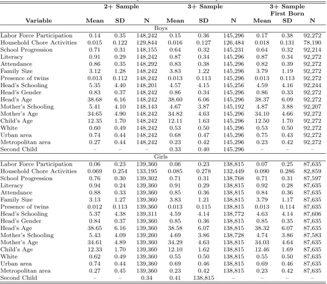
Table (1) presents the descriptive statistics of the 2+, 3+, and 3+ - first-born samples for the
ten-to-fifteen-year age group for boys and girls separately. We notice that labor-force participation
for boys is almost twice as large as that of girls. For instance, in the 2+ sample, 14% of all
boys participate in the labor market, whereas 6% of all girls are participants in the labor market.
Conversely, the incidence of household-chore activities is greater among girls compared to boys. Of
all first-born girls who are not participating in the labor market, 7% report doing some chores in
the 2+ sample. This figure is 1.5% for boys. Regarding educational outcomes, 85% of the boys and
87% of the girls are attending school in the 2+ sample. As is commonly observed in developing
countries, children experience some school delays. This phenomenon occurs for both boys and girls
and is slightly more frequent among boys. The average school progression indices are 0.71 and 0.76
for boys and girls in the 2+ sample, respectively. Finally, 91% of the boys and 94% of the girls in
the 2+ sample are literate. Of all families with two or more births, 1.3% have twins in the second
birth. The same figure appears in the 3+ sample. The average family size is 3.1 for the 2+ sample
and 3.8 for the 3+ sample. Approximately 74% live in urban areas in the 2+ sample and 69% in
the 3+ sample.
[INSERT TABLES 1 AND 2 HERE]
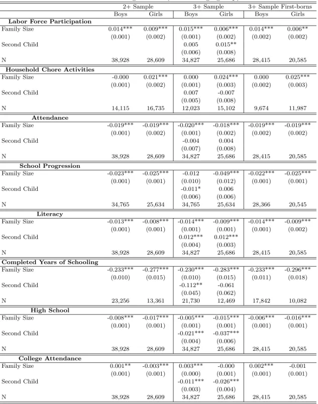
Table 3 presents the OLS regression results for all three samples of the ten-to-fifteen age group.
They are qualitatively the same for boys and girls. All show positive and significant coefficients of
family size on labor-force participation and household chores. Negative and significant coefficients
are also observed for attendance, school progression and literacy.
Overall, the OLS results indicate that individuals in larger families are more prone to engage in
labor-market activities and chores (especially girls) and present lower educational outcomes. These
[INSERT TABLES 3 AND 4 HERE]
Are these results reliable? First, we check whether the IV has a strong correlation with the
potential endogenous variable. Table 5 displays the first-stage results of the IV regressions for the
ten-to-fifteen age group. All coefficients of the instrument are positive and statistically significant.
We also notice that families whose child is white, whose parents are more educated, and who live
in urban and metropolitan areas have fewer children (not shown in the tables). The same results
are obtained in the first-stage regressions of the eighteen-to-twenty-year age group and are shown
in Table 6 below.
Some observations are worth noting. First, the measure of the number of siblings is accurate
in our samples because we exclude all families that have some children who are deceased or living
outside the household. In other words, we include complete families only. Second, our
measure-ment of the presence of twins may be overestimated because we identify twins by the age of the
individuals. Therefore, it is possible that some non-twin siblings are misclassified as twins, which
might generate measurement errors in our instrumental variable. However, as long as they are
not correlated with the error in the second-stage equation and the measure of presence of twins is
correlated to the actual variable, the second-stage coefficients are consistent even if they bias the
first-stage coefficients.
[INSERT TABLES 5 AND 6 HERE]
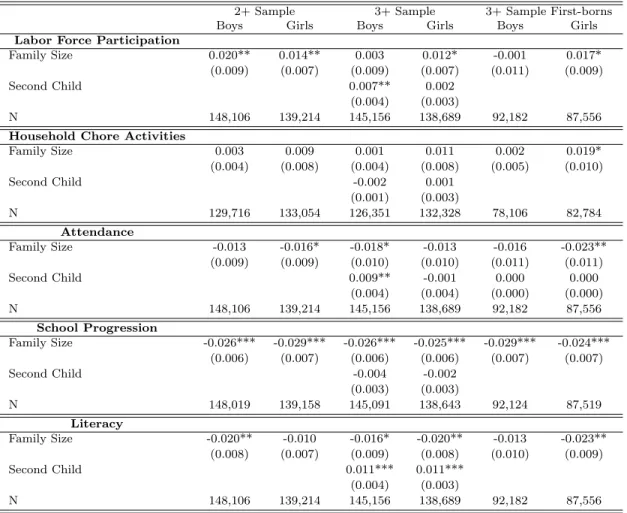
The IV second-stage regressions for the ten-to-fifteen-year age group displayed in Table 7 show
the impacts of family size on child-quality outcomes for boys and girls separately. The results for
labor-force participation show a positive and significant impact of family size in the three different
samples for girls. For boys, only the coefficient in the 2+ sample is statistically significant. The IV
point estimates imply that an extra sibling increases the likelihood of a girl (boy) joining the labor
market by 1.4 (2.0) percentage points in the 2+ sample. This increase is sizeable. The child labor
Brazil, which implies that an extra sibling increases the probability of a child working by 1.4/6=23%
for girls and 2.0/14=14% for boys. The results for the 3+ samples are also positive and significant,
with similar magnitudes for girls. However, they are not statistically significant for boys15.
The results for household chores are not statically significant, except for the values for girls
in the 3+ firstborn sample. It is important to notice that the definition of household chores is
narrow and consists of a full-time activity for those are who not participating in the labor market.
16 It is possible that individuals engage in household chores combined with other activities and
that this is more likely to occur in larger families. However, we cannot capture this impact due to
the definition of household chores used in the Census. Nevertheless, it is interesting to notice that
there is a positive and significant impact of family size for first-born girls in the 3+ sample, which
may suggest a process in the intra-household allocation decisions in which older females in larger
families dedicate more time to taking care of younger siblings and/or household duties. The fact
that we did not find this effect in the 2+ sample indicates that the impact may be non-linear with
respect to family size.
The results for school attendance suggest a detrimental effect of family size. The coefficient
is statistically different from zero at a 5% level of significance for girls in the 3+ firstborn sample
only. However, all of the coefficients are negative, and point estimates range from -1.3 to -2.3
percentage points. For the first-born girls in the 3+ sample, an extra sibling reduces the probability
of attending school by 2.3 percentage points, which corresponds to an increase of 2.3/14.81=15.5%
for the probability of not attending school.
For school progression, the results indicate a detrimental effect of family size. The coefficients
are negative and significant for boys and girls and for all samples, and they imply a considerable
effect on educational attainment. For instance, the point estimate for girls in the 2+ sample is
approximately 0.03. The average school progression is approximately 0.9. If a fifteen-year-old girl
15
We also investigate the impact of family size on work intensity. We observe the intensive margin by including weekly working hours as an additional outcome. We did not find any impact of family size on this margin. The results are available upon request.
16
is in the correct grade, she must have nine years of schooling. The marginal impact of family size
would decrease this figure to 9 x 0.03 = 0.27 years of schooling, i.e., one-third of a year of schooling.
Indeed, there is evidence that a school delay is associated with lower final educational attainments
(see, for instance, Meisels and Liaw (1993) and Bedi and Marshall (2002)).
Finally, for literacy, we find negative point estimates of family size. For girls, the results are
significant in the 3+ samples only. For boys, family size is not significant in the 3+ firstborn sample
only. For instance, boys in the 2+ sample are impacted by a decrease of two percentage points in
the probability of being literate. This magnitude implies that an extra sibling increases the chances
of being illiterate by 2/9 = 22%.
[INSERT TABLE 7 HERE]
When comparing the IV with the OLS regressions, the OLS coefficients seem to overestimate
(in absolute terms) the actual impact of family size on household chores, school attendance, school
progression, and literacy outcomes for both boys and girls. However, in the case of labor-force
participation, the OLS biases are different for boys and girls. For boys, the OLS bias is positive.
The opposite occurs for girls, even though the point estimates of OLS and IV are similar. These
comparisons suggest that families with a preference for child quantity care less about child quality
or are more likely to be credit-constrained. The same bias direction for both boys and girls for
most of the outcomes suggests that unobservable tastes, wealth, and ability are similarly correlated
with girls’ and boys’ outcomes. The twins IV approach accounts for these biases.
Impacts on the Eighteen-to-Twenty-Year Age Group
The tradeoff between the quantity and quality of children may cause lasting effects on individual
human capital accumulation. Ideally, to measure these completed impacts, we want to observe
the adult siblings after completion of their human capital formation. Although no such data
are available in Brazil, we can observe young adults still living with their parents and siblings.
the young adult sample involves a tradeoff. An older young adult is more likely to have completed
the human capital formation but is less likely to still live with the parents and siblings. To maximize
the number of individuals who still live with their parents and have completed their formal education
process, we choose the eighteen-to-twenty-year age range. In fact, approximately 70% of the
18-20-year age-group individuals live in the same household as their parents. Moreover, of all
eighteen-to twenty-year-old individuals, 70% were not attending school in 1991. It is important eighteen-to notice
that females generally move out of their parents’ household earlier than males to become spouses.
Of all individuals who still live with their parents, 58% are males, and 42% are females.
Similar to the 10-15-year age group, we construct three different samples for the 18-20-year age
group. Table (2) presents the descriptive statistics of the 2+, 3+ and 3+ - firstborn samples for
boys and girls separately. In the 2+ sample, 70% of all males and 46% of the females participate in
the labor market. Of all females who are not participating in the labor market, roughly 24% report
doing some chores in the 2+ sample. This figure is 4.5% for males. In total, 40% of the males and
53% of the females are attending school in the 2+ sample17. The average school progression indices
are 0.57 and 0.68 for males and females in the 2+ sample, respectively. In total, 93% (96%) of the
males (females) in the 2+ sample are literate. We construct three additional outcomes of this age
group. The first one is the an indicator variable if the individual completed high school.18 The
second is an indicator variable if the individual has attended college. Finally, for those who are not
attending school anymore, we obtain the completed years of schooling. The goal is to capture the
completed human capital formation. For high school completion, 17% (28%) of the males (females)
have completed high school in the 2+ samples. For the 3+ sample, the figures for high school
completion are 13% and 22% for males and females, respectively. For college attendance, 8% (15%)
and 13% (22%) of the males (females) attend college in the 2+ and 3+ samples, respectively. For
those who are not attending school, the average completed years of schooling is 6.4 (7.4) in the
17
These figures are different from the population averages because the sample is restricted to sons and daughters living with their parents. We observe that they are more likely to attend school compared to those who live outside the parents’ household.
18
2+ sample. Of all families in the 2+ sample, 1.4% have twin births in the second birth. A similar
number is obtained for the 3+ sample. The average family size is approximately 3.6 for the 2+
sample and 4.3 for the 3+ sample. Roughly 74% live in urban areas in the 2+ sample, and 70%
live in urban areas in the 3+ sample.
Table 4 presents the OLS regression results for all three samples in the
eighteen-to-twenty-year age group. The outcomes of child labor and education remain qualitatively similar to those
found for the ten-to-fifteen-year age group, except for household chores, which present statistically
insignificant coefficients for males. Particularly important is that an extra sibling is associated with
a lower probability of completing high school. This result holds for boys and girls for all samples.
For college attendance, we find that family size is positively correlated with the probability of a
male attending college. However, this correlation is negative for females in the 2+ sample. Finally,
an extra sibling is associated with -0.23 (-0.28) completed years of schooling for males (females).
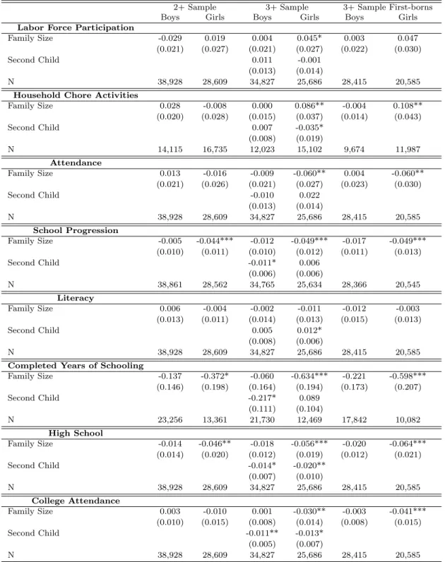
Tables 6 and 8 present the first-and second-stage results. The first-stage results depict a strong
positive correlation between the presence of twins and family size for all samples. The second-stage
regressions show no impact of family size on labor-force participation and household chores for boys.
For girls, they show a positive impact on these outcomes for the 3+ sample. Indeed, the regressions
are statistically significant for household chores. The impact is considerable. For instance, the
coefficient in the 3+ firstborn sample is 0.108, which implies an increase in the probability of doing
chores by 0.108/0.265 = 40.7%.
The same pattern is observed for school attendance and progression, high school completion and
college attendance. There are no impacts of family size for boys, but there are significant effects
for girls. For school and college attendance, the results are significant for the 3+ sample, and
the estimated coefficients are 0.06 and 0.04, respectively, for the firstborn females, which implies a
decrease of 0.06/0.51 = 11.8% and of 0.04/0.12 = 30%, respectively, in the probability of attending
school and college. There is a significant impact on school progression and high school completion
for females in all three samples. For literacy, the results show no significant impact for males or
Finally, the results reveal a negative and significant effect of family size on the completed years
of schooling for females. Although the value is negative, there is no significant impact for males.
For females in the 3+ firstborn sample, the estimated coefficient is -0.598, showing that an extra
sibling reduces the expected completed formal education by more than half a year.
Compared to the OLS results, the IV estimations generate higher point estimates for girls (in
absolute values) and lower point estimates, in most cases, for boys in the young adults age group.
One possible explanation is that there is a household specialization among siblings, particularly
for credit-constrained families. An unexpected extra sibling forces them to gender-specialize even
more. The results suggest that those families invest more in the human capital formation of the
oldest male, while the females specialize in doing household chores to the detriment of schooling
investments. The IV may be capturing this specialization forced by the unexpected child.
Taken together, these results indicate that the tradeoff between quantity and quality implies
time-allocation choices that are detrimental for females, especially for those in larger families.
In general, it seems that they have a lower probability maintaining the process of human capital
accumulation, and those who have completed this process end up completing less years of schooling.
Moreover, they are more likely to do household chores as their main time-allocation activity.
[INSERT TABLE 8 HERE]
Mechanisms
There are two plausible conjectures about the mechanisms through which the family size impacts
human capital formation: credit and time constraints. The credit-constraint channel operates
through the dilution of income resources due to the birth of the extra sibling. The impossibility
of bringing the family’s future income to the present may reduce the amount of resources available
to each family member. Therefore, to maintain current consumption, this constraint may force the
family to under-invest in the human capital formation of the children and to push them to the
The time-constraint channel works through the dilution of time devoted by parents to each
child after the birth of the extra sibling. The birth of a new sibling may restrict the time that
the parents allocate to the raising of each child. This restriction may cause a reallocation of the
time of the parents and of the older siblings to take care of the younger siblings. This restriction
may impact the children’s human capital formation in two ways. First, parents may dedicate less
time to the care and education of each child. Second, the family may require the use of time of
some children, especially the older ones, in activities that might be detrimental to their own human
capital formation, such as labor market activities, taking care of the younger siblings, or other
chores.
This subsection sheds some light on these possible channels. First, to investigate the
exis-tence of the credit-constraint channel, we divide the sample between families with low- and
high-educated mothers. We define low-high-educated mothers as those with three or less years of schooling
and high-educated mothers as those with eleven or more years of schooling. The assumption is
that the mother’s education is correlated with the family’s wealth. If wealthy families are less
credit-constrained, then the mother’s education may be a good indicator of how likely a family is
to be credit-constrained.19
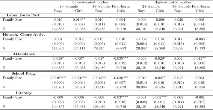
The results are presented in tables 9 and 10 for the ten to fifteen and eighteen to twenty age
groups, respectively. We find evidence that suggests that the credit-constraint channel is, indeed,
a relevant mechanism through which the quantity and quality tradeoff operates. We find that the
detrimental effects on schooling are more pervasive among low-educated mother families.
[INSERT TABLES 9 AND 10 HERE]
Second, we analyze the presence of the time-constraint channel by exploring the differences in
the exposure time of the firstborn sibling to the occurrence of an unexpected extra birth in the
family. This mechanism may operate in different ways. For instance, consider the cases of two
firstborn children that are both exposed to an extra sibling. In the first case, the child is ten
19
years old, and in the second case, the child is two years old. On the one hand, the parents of the
ten-year-old can devote more years to the sole care of the firstborn child compared to the parents of
the two-year-old child. This can have different accumulative effects in the human capital formation
of the children. On the other hand, the larger age gap may make the firstborn child more likely
to engage in activities that steal time from her own human capital accumulation, such as taking
care of the younger sibling and doing household chores. Therefore, the net effect of an extra sibling
through this channel is ambiguous. Moreover, these effects may be non-linear. The age gap between
the two siblings might be sufficiently wide that the human capital accumulation process is already
completed.
We investigate the presence of the time-constraint channel by dividing the sample into narrow
and wide-birth spacing groups. The narrow-spacing group is formed by firstborn children living in
families in which the difference between the first birth and the births of twins is equal to or less than
two years. The wide-spacing group is formed by firstborn in families in which the difference between
the first birth and the births of twins is greater than two years. The time-constraint channel is
inferred by comparing the impacts of family size in the narrow and wide-spacing samples, controlling
for the firstborn child’s age. Therefore, the difference in spacing captures the difference in the age of
exposure to the increase in the family size between both samples. The results are presented in tables
11 and 12. Overall, we find an increase in the family size tends to affect more firstborn children in
the wide-spacing group. Family size is detrimental to school progression for the children aged 10-15
years in wide-spacing families. For the 18-20 age group, the family size negatively impacts most of
the educational outcomes of firstborn girls in wide-spacing families in the 3+ sample. Moreover,
there is also a positive impact on the likelihood of doing household chores for firstborn girls in the
3+ sample.
These results suggest that both mechanisms (credit and time constraints) may be acting to
explain the impacts of family size in child quality outcomes. In the presence of gender specialization,
the credit- and time-constraint channels seem to negatively impact the educational attainment of
are more affected by an extra sibling, it seems that the time-constraint channel occurs through the
time reallocation of the older sibling.
[INSERT TABLES 11 AND 12 HERE]
6
Conclusion
In this paper, we estimate the causal impact of family size on new dimensions of child quality.
Specifically, we gauge the effect of an extra sibling on child labor, an often-neglected outcome that
is closely related to children’s well-being. We use two distinct indicators: labor-force participation
and household chores. We also investigate the effects on more traditional educational outcomes,
such as school attendance, school progression, and literacy outcomes. We observe two age groups.
The first outcome encompasses children aged between 10 and 15 years. To check possible lasting
effects of family size, we also analyze the impacts on young adults aged 18 to 20 years. For
the second age group, we additionally estimate the impact on high school completion, college
attendance and the completed years of schooling for those who have completed their formal human
capital accumulation.
The main empirical problem in measuring such an effect is the potential endogeneity of fertility,
as it is a choice variable, and unobservables might influence both family-size choice and
child-quality outcomes. To overcome this problem, we use the instrumental variable estimation approach.
We use the presence of twins as the instrument for family size. We show that the presence of
twins is strongly correlated with the number of children. Because the birth of twins is very likely
to be a random event and orthogonal to the unobservables that may affect children and family
characteristics, we believe that the presence of twins has the required properties to be a good
instrumental variable.
A simple OLS approach shows a strong detrimental relationship between family size and
child-quality outcomes. The IV estimators reveal that the OLS coefficients are upward-biased. They also
boys and girls and to household chores for young women. Moreover, we find negative effects on
educational outcomes for boys and girls and negative impacts on human capital formation for young
female adults. Indeed, the results show that young women suffer most of the detrimental impact
of an extra sibling, particularly in larger families. They are more likely to work domestically, less
likely to attend school, more likely to lag further behind in school, and more likely to complete
fewer years of schooling.
Unlike studies that focus on developed countries, our study shows detrimental effects on
edu-cational outcomes for both boys and girls as well as young females. The difference in the findings
may be related to developing-country contexts, where credit rationing is more pervasive. Therefore,
the quantity-quality tradeoff is measurable. An extra child may impose a larger resource dilution
without the possibility of consumption smoothing over time in a family. In this situation, fewer
resources may be allocated to other siblings. In particular, the time endowment of young women
may be reallocated to domestic work rather than to their own human capital accumulation. Indeed,
we find evidence that suggests that both credit and time constraints are important mechanisms of
the family-size effects on child quality.
These results can help to improve the design of anti-poverty programs in developing countries.
For instance, conditional cash transfer programs are widespread across developing countries. Such
a program usually consists of cash transfers that are conditional upon school attendance and/or
visits to health care centers. The value of the transfers generally depends on the number of children
in the family. A family with more children is eligible to receive greater cash transfers. If our results
are correct, then the positive effect of the program on child-quality outcomes can be offset by the
potential incentive of higher fertility.
Finally, the results suggest that there is gender specialization inside the family when a newborn
arrives. Older female children in larger families seem to dedicate more time to taking care of
younger siblings and/or to household duties, thereby jeopardizing their long-term human capital
References
Angrist, Joshua D and William N Evans, “Children and Their Parents’ Labor Supply:
Ev-idence from Exogenous Variation in Family Size,” American Economic Review, June 1998, 88
(3), 450–77. available at http://ideas.repec.org/a/aea/aecrev/v88y1998i3p450-77.html.
Angrist, Joshua D., Victor Lavy, and Analia Schlosser, “New Evidence on the
Causal Link Between the Quantity and Quality of Children,” NBER Working
Pa-pers 11835, National Bureau of Economic Research, Inc December 2005. available at
http://ideas.repec.org/p/nbr/nberwo/11835.html.
, , and , “Multiple Experiments For The Causal Link Between The Quantity And Quality Of
Children,” Technical Report, Massachusetts Institute of Technology Department of Economics
Working Paper Series 2006.
Baland, Jean-Marie and James A. Robinson, “Is Child Labor Inefficient?,”
Journal of Political Economy, August 2000, 108 (4), 663–679. available at
http://ideas.repec.org/a/ucp/jpolec/v108y2000i4p663-679.html.
Basu, Kaushik, “Child Labor: Cause, Consequence, and Cure, with Remarks on International
Labor Standards,”Journal of Economic Literature, September 1999,37(3), 1083–1119. available
at http://ideas.repec.org/a/aea/jeclit/v37y1999i3p1083-1119.html.
Becker, Gary S and H Gregg Lewis, “On the Interaction between the Quantity and
Qual-ity of Children,” Journal of Political Economy, Part II, 1973, 81 (2), S279–88. available at
http://ideas.repec.org/a/ucp/jpolec/v81y1973i2ps279-88.html.
and Nigel Tomes, “Child Endowments and the Quantity and Quality of
Chil-dren,” Journal of Political Economy, August 1976, 84 (4), S143–62. available at
Bedi, Arjun S. and Jeffery H. Marshall, “Primary school attendance in Honduras,” Journal
of Development Economics, October 2002,69(1), 129–153.
Beegle, Kathleen, Rajeev Dehejia, and Roberta Gatti, “Why should we care about child
labor? The education, labor market, and health consequences of child labor,” Policy Research
Working Paper Series 3479, The World Bank January 2005.
, Rajeev H. Dehejia, and Roberta Gatti, “Child labor and agricultural shocks,”
Journal of Development Economics, October 2006, 81 (1), 80–96. available at
http://ideas.repec.org/a/eee/deveco/v81y2006i1p80-96.html.
Behrman, Jere R. and Mark R. Rosenzweig, “Returns to Birthweight,” The Review of
Economics and Statistics, 06 2004, 86(2), 586–601.
Black, Sandra E., Paul J. Devereux, and Kjell G. Salvanes, “The More the
Merrier? The Effect of Family Size and Birth Order on Children’s Education,”
The Quarterly Journal of Economics, May 2005, 120 (2), 669–700. available at
http://ideas.repec.org/a/tpr/qjecon/v120y2005i2p669-700.html.
Blau, Francine D and Adam J Grossberg, “Maternal Labor Supply and Children’s Cognitive
Development,” The Review of Economics and Statistics, August 1992,74 (3), 474–81. available
at http://ideas.repec.org/a/tpr/restat/v74y1992i3p474-81.html.
Borlot, Ana Maria Monteiro and Zeidi Ara´ujo Trindade, “As tecnologias de reprodu¸c˜ao
assistida e as representa¸c˜oes sociais de filho biol´ogico,” Estudos de Psicologia, 2004, 9, 63–70.
Caceres-Delpiano, Julio, “The Impacts of Family Size on Investment in Child Quality,” J.
Human Resources, 2006,XLI(4), 738–754.
Cigno, Alessandor and Camillo Rosati, “Child Labour Education and Nutrition in Rural
and ,The Economics of Child Labor, Oxford University Press,
Conley, Dalton and Rebecca Glauber, “Parental Educational Investment and Children’s
Aca-demic Risk: Estimates of the Impact of Sibship Size and Birth Order from Exogenous Variations
in Fertility,” May 2005, (11302). available at http://ideas.repec.org/p/nbr/nberwo/11302.html.
Deb, P. and C. Rosati, “Estimating the Effect of Fertility Decisions on Child Labour,” February
2004. available at http://ideas.repec.org/p/ucw/worpap/4.html.
Edmonds, Eric V., Child Labor, Vol. 4 of Handbook of Development Economics, Elsevier,
De-cember
and Nina Pavcnik, “Child Labor in the Global Economy,” Journal of Economic Perspectives,
Winter 2005, 19(1), 199–220. available at
http://ideas.repec.org/a/aea/jecper/v19y2005i1p199-220.html.
and , “International trade and child labor: Cross-country evidence,”
Jour-nal of International Economics, January 2006, 68 (1), 115–140. available at
http://ideas.repec.org/a/eee/inecon/v68y2006i1p115-140.html.
Emerson, Patrick M. and Andre Portela Souza, “Is Child Labor Harmful? The Impact of
working Earlier in Life on Adult Earnings.,” 2011. Economic Development and Cultural Change,
forthcoming.
Goux, Dominique and Eric Maurin, “The effect of overcrowded housing on children’s
per-formance at school,” Journal of Public Economics, June 2005, 89 (5-6), 797–819. available at
http://ideas.repec.org/a/eee/pubeco/v89y2005i5-6p797-819.html.
Haan, Monique De, “Birth Order, Family Size and Educational Attainment,” Tinbergen
Institute Discussion Papers 05-116/3, Tinbergen Institute December 2005. available at
Hanushek, Eric A, “The Trade-Off between Child Quantity and Quality,”
Journal of Political Economy, February 1992, 100 (1), 84–117. available at
http://ideas.repec.org/a/ucp/jpolec/v100y1992i1p84-117.html.
Lee, Jungmin, “Sibling Size and Investment in Children’s Education: An Asian Instrument,”
September 2004, (1323). available at http://ideas.repec.org/p/iza/izadps/dp1323.html.
Li, Hongbin, Junsen Zhang, and Yi Zhu, “The Quantity-Quality Tradeoff of Children in a
Developing Country: Identification Using Chinese Twins,” August 2007, (3012).
Meisels, Samuel J. and Fong-Ruey Liaw, “Failure in Grade: Do Retained Students Catch
Up?,” The Journal of Educational Research, 1993,87, 69–77.
Orazem, Peter F. and Chanyoung Lee, Research in Labor Economics, Vol 31: Child Labor
and the Transition Between School and Work, Emerald Group Publishing Limited,
Psacharopoulos, George and Harry Anthony Patrinos, “Family size, schooling and child
labor in Peru - An empirical analysis,”Journal of Population Economics, 1997, 10(4), 387–405.
available at http://ideas.repec.org/a/spr/jopoec/v10y1997i4p387-405.html.
Qian, Nancy, “Quantity-Quality and the One Child Policy: The Only-Child Disadvantage on
School Enrollment in Rural China,” Technical Report 2008.
Rosenzweig, Mark R and Kenneth I Wolpin, “Testing the Quantity-Quality Fertility Model:
The Use of Twins as a Natural Experiment,” Econometrica, January 1980, 48 (1), 227–40.
Figures and Tables
Table 1: Summary statistics - 10 to 15 years old
2+ Sample 3+ Sample 3+ Sample First Born Variable Mean SD N Mean SD N Mean SD N
Boys
Labor Force Participation 0.14 0.35 148,242 0.15 0.36 145,296 0.17 0.38 92,272 Household Chore Activities 0.015 0.122 129,844 0.016 0.127 126,484 0.018 0.131 78,190 School Progression 0.71 0.31 148,155 0.64 0.32 145,231 0.64 0.32 92,214
Literacy 0.91 0.29 148,242 0.87 0.34 145,296 0.87 0.34 92,272
Attendance 0.86 0.35 148,292 0.83 0.38 145,296 0.82 0.39 92,272
Family Size 3.12 1.28 148,242 3.83 1.22 145,296 3.79 1.19 92,272
Presence of twins 0.013 0.112 148,242 0.013 0.113 145,296 0.013 0.113 92,272 Head’s Schooling 5.35 4.40 148,201 4.57 4.15 145,256 4.59 4.16 92,244
Head’s Gender 0.83 0.37 148,242 0.86 0.34 145,296 0.86 0.33 92,272
Head’s Age 38.68 6.16 148,242 38.60 6.06 145,296 38.37 6.09 92,272
Mother’s Schooling 5.41 4.10 148,143 4.67 3.87 145,192 4.87 3.88 92,207 Mother’s Age 34.65 4.90 148,242 34.82 4.63 145,296 34.10 4.66 92,272 Child’s Age 12.35 1.70 148,242 12.11 1.63 145,296 12.50 1.70 92,272
White 0.60 0.49 148,242 0.53 0.50 145,296 0.53 0.50 92,272
Urban area 0.74 0.44 148,242 0.68 0.47 145,296 0.75 0.43 92,272
Metropolitan area 0.27 0.44 148,242 0.23 0.42 145,296 0.23 0.42 92,272
Second Child – – – 0.33 0.40 145,296 – – –
Girls
Labor Force Participation 0.06 0.23 139,360 0.06 0.23 138,815 0.07 0.25 87,635 Household Chore Activities 0.069 0.254 133,195 0.085 0.278 132,449 0.090 0.286 82,859 School Progression 0.76 0.30 139,302 0.71 0.31 138,768 0.71 0.31 87,597
Literacy 0.94 0.24 139,360 0.91 0.29 138,815 0.92 0.28 87,635
Attendance 0.88 0.33 139,360 0.85 0.36 138,815 0.84 0.36 87,635
Family Size 3.13 1.27 139,360 3.83 1.21 138,815 3.79 1.17 87,635
Presence of twins 0.012 0.113 139,360 0.013 0.115 138,815 0.013 0.114 87,635 Head’s Schooling 5.37 4.38 139,311 4.59 4.14 138,772 4.63 4.14 87,606
Head’s Gender 0.84 0.37 139,360 0.85 0.36 138,815 0.85 0.35 87,635
Head’s Age 38.65 6.16 139,360 38.58 6.07 138,815 38.32 6.07 87,635
Mother’s Schooling 5.43 4.09 139,260 4.69 3.86 138,728 4.74 3.86 87,583 Mother’s Age 34.61 4.89 139,360 34.29 4.63 138,815 34.03 4.64 87,635 Child’s Age 12.33 1.70 139,360 12.10 1.62 138,815 12.46 1.69 87,635
White 0.62 0.49 139,360 0.55 0.50 138,815 0.55 0.50 87,635
Urban area 0.74 0.44 139,360 0.69 0.46 138,815 0.69 0.46 87,635
Metropolitan area 0.27 0.45 139,360 0.23 0.42 138,815 0.23 0.42 87,635