Article
Improving cluster-based methods for investigating potential for insect pest
species establishment: region-specific risk factors
Michael J. Watts1, Susan P. Worner2
1
School of Earth and Environmental Sciences, University of Adelaide, North Terrace, SA 5005, Australia
2
Bio-Protection Research Centre, Lincoln University, PO Box 84, Lincoln 7647, New Zealand E-mail: mjwatts@ieee.org
Received 9 May 2011; Accepted 7 June 2011; Published online 1 September 2011 IAEES
Abstract
Existing cluster-based methods for investigating insect species assemblages or profiles of a region to indicate
the risk of new insect pest invasion have a major limitation in that they assign the same species risk factors to each region in a cluster. Clearly regions assigned to the same cluster have different degrees of similarity with respect to their species profile or assemblage. This study addresses this concern by applying weighting factors
to the cluster elements used to calculate regional risk factors, thereby producing region-specific risk factors. Using a database of the global distribution of crop insect pest species, we found that we were able to produce
highly differentiated region-specific risk factors for insect pests. We did this by weighting cluster elements by their Euclidean distance from the target region. Using this approach meant that risk weightings were derived that were more realistic, as they were specific to the pest profile or species assemblage of each region. This
weighting method provides an improved tool for estimating the potential invasion risk posed by exotic species given that they have an opportunity to establish in a target region.
Keywords data clustering; k-means clustering; invasive insect pests; regional species assemblages.
1 Introduction
Pre-emergence risk evaluation, that is, evaluating which species of insect crop pest are most likely to invade a
geographic region (Worner and Gevrey, 2006; Zhang, 2010), can be carried out using data clustering (Paini et al, 2010; Watts and Worner, 2009).
Data clustering (Everitt, Landau and Leese, 2001) is an important and widely used method of data analysis
that groups similar items together into subsets, or clusters, made up of a number of elements where each item in a cluster is more similar with respect to its elements to the other items in the cluster than it is to items outside the cluster. By determining the cluster which a geographical region, as represented by its species
assemblage, belongs to, it may be possible to infer which pest species may become established in that region (Watts and Worner, 2009; Worner and Gevrey, 2006; Gevrey et al, 2006). Such inference is based on the
concept that regions that have similar assemblages or species profiles are likely to have climatic or other environmental properties in common that allow the particular mix of species to establish. If the region of interest (the target region) in a cluster does not have a species present, yet that species is present in a large
the establishment of that species, if it were to be accidentally introduced or arrive by independent means in the target area. By measuring the frequency at which a species appears in a cluster, a quantitative “risk weighting”
or “risk value” can be derived. This has previously been calculated as a simple unweighted arithmetic mean across all assemblages present in the cluster in which the target region appears (the “target cluster”) (Watts and Worner, 2009). An alternative clustering method is to use the weights from a self-organising map (SOM)
analysis as a measure of the risk value (Gevrey et al, 2006).
A significant criticism of this approach is that all assemblages in a cluster are considered equal. That is, if an assemblage is in a target cluster, then the contribution of that assemblage to the final species ranking is the
same as all other assemblages in that cluster, no matter the actual degree of similarity of that assemblage to the assemblage associated with the target cluster. A consequence of this is that the species risk weightings of all species for all regions in a cluster are equal. Equal similarity of all species assemblages in a cluster is of course
not realistic.
The work presented in Watts and Worner, (2009) demonstrated that, for the task of clustering a specific database of insect pest assemblages (CABI, 2003), k-means clustering (Lloyd, 1982) produced similar clusters
that were of superior quality to those produced by Kohonen Self-Organizing Maps (SOM) (Kohonen, 1990) as determined by objective cluster measures. Additionally, its computational efficiency was many orders of
magnitude greater than that of a SOM. These clusters were used to produce ranked risk-lists of the species posing the greatest threat of invasion to New Zealand. Because of its good performance on this dataset and its computational efficiency, k-means was used for the analysis in this study.
The motivation for the work described in this paper was to address the criticism above by weighting
contributions of the final species risk values by the similarity of each member of the target cluster to the target regions assemblage. The clusters produced by the k-means algorithm in Watts and Worner (2009) above were
reanalysed using weighting factors for the assemblages and clusters, and new risk lists produced that are specific to New Zealand. The ranks of species within these risk lists were then compared to the original ranks and to the species ranks of another region, Tasmania, which was clustered within the same cluster as New
Zealand in the previous analysis, so that any differences resulting from the weighting became apparent.
2 Method
2.1 Generating the original clusters
Here we briefly describe the data and methods used to generate the source clusters. For a comprehensive description of these methods, please see Watts and Worner, (2009).
The data that was clustered in this work was sourced from the CABI Crop Protection Compendium 2003
(CABI, 2003). The data described the presence and absence of 844 phytophagous crop pest species within 459 geopolitical regions, which represented the entirety of the world’s landmass, excluding Antarctica. Each region was thus represented by an 844 element binary vector, where each element represents the presence (1) or
absence (0) of a species. Species were included in the data set only if they were present in more than 5% of the geographic regions. The species assemblages were verified as non-random via null-model analysis (Gotelli,
2000) and k-means clustering (Lloyd, 1982) was performed. One thousand independent k-means clustering sessions were carried out. While Kohonen SOM (Kohonen, 1990) was also investigated in Watts and Worner (2009), that work determined that k-means yielded superior results. That is, for this data set, k-means yielded
clusters of superior quality as measured by objective cluster measures, compared to SOM. Therefore, the SOM results were not re-examined in this work. The weighting technique presented here, however, makes no
clustering method. The method also does not make any assumptions about the species being clustered: while most of the published material so far has been on insects, recent work (Watts, 2011) has shown that it can also
be applied to assemblages of bacterial crop diseases. No work has yet been done, however, on mixed assemblages, for example, assemblages of plants and insects.
2.2 Generating risk lists
The goal of the experiments reported here was to generate using k-means clustering lists of insect pest species that were ordered according to the risk they pose to the target region, which in this case was New Zealand. There appears to be no reason this method could not be applied to other regions, and a SOM-based version of
this technique has since been applied to Australia (Paini et al, 2010). New Zealand was chosen as the target region because the research was carried out at a New Zealand university, partially funded by a New Zealand government grant. The fundamental assumption made with this technique is that regions that have similar
environmental conditions will probably have similar species assemblages. Therefore, the risk of a species establishing can be determined from the frequency at which it appears in assemblages that are similar to the
target assemblage: a higher frequency means it is present in more regions, which means it is more able to establish in regions that are similar to the target region. The work reported in Paini et al (2010) found a high level of concordance between the ranks derived using this method and the ranks assigned to species by domain
experts. The algorithm for finding risk rankings from clusters is based on that assumption, and is as follows:
for each trial
o find the cluster the target region is in (the target cluster)
o identify all regions that are in the target cluster (the neighbour regions)
o calculate the frequency each species appears in the target cluster, where the frequency is the
mean of species presence across the assemblages belonging to the neighbour regions (the risk
weightings)
o use these frequencies to calculate the ranks of each species, where higher-frequency species
rank more highly than species with lower frequencies
calculate the mean of the ranks for each species
order species by their mean ranks
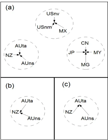
The conceptual diagram in Fig. 1(a) shows how the risk factors are derived from the assemblage clusters.
Rankings are assigned in descending order1. Species with the same risk values are given an average ranking.
For example, if three species with the same risk values are ranked 18, 17 and 16, each will be given the rank of
17, and the following species assigned the rank 15 (unless that species also shares a risk value with other species). The final rankings are determined as the mean of the ranked risk-lists from each of the clustering runs. It should be self-evident that this algorithm will assign a higher mean rank to species that appear more
frequently in the same cluster as the target region.
Generating risk weightings by this method results in rankings that are the same for all regions in the cluster. That is, the risk ranking assigned to each species is the same for each region in the target cluster, no matter
how similar or dissimilar the species profile or the environment in that region is to that of the target region. This problem can be addressed by weighting the contribution each assemblage makes to the risk factors.
1
This is for consistency with the previous work (Watts and Worner, 2009; Worner and Gevrey, 2006). Obviously, ranks could be
assigned in ascending order without affecting the results presented here beyond high-risk species getting lower ranks than low
Weighted risk lists were generated by applying weighting factors to the species assemblages present in the target cluster for each rep, then calculating the unweighted mean risk values across all of the reps (that is,
weighting the assemblages). This process is shown in conceptual form in Fig. 1. The weights applied to the assemblages were the inverse of the Euclidean distance between each assemblage and the target assemblage, that is, assemblages that were more similar to the target assemblage contributed more to the risk weighting
than assemblages that were less similar to the target assemblage. While any similarity measure could have been used to generate weighting factors (such as Jaccard similarity, Manhattan distance or the simple similarity
coefficient (Krebs, 1999)), Euclidean distance was used because this was the measure used to perform the clustering.
Fig. 1 Conceptual diagram of risk value calculation process. In (a) unweighted values are found as the centres of clusters. In (b) risk values are weighted towards the NZ (New Zealand) region. In (c) risk values are weighted towards the AUta (Tasmania) region.
The weighted mean was calculated according to Equation 1:
(1)
where, is the presence or absence of species i is the current cluster, where presence is represented by unity
weighting factor was the inverse of the Euclidean distance between the current and target assemblage, as in Equation 2:
(2)
where is the Euclidean distance between assemblage i and the target assemblage t.
2.3 Comparison with neighbour regions
In the k-means clustering reported in Watts and Worner (2009), the region other than New Zealand that
appeared the most in the target cluster was Tasmania. Since the major criticism of the unweighted risk-generation approach was that every region in the target cluster has the same risks derived, a comparison was
carried out between the weighted risks for New Zealand and the weighted risks for Tasmania. Ranks were derived for New Zealand and Tasmania only using clusters where both New Zealand and Tasmania were
present. That is, trials where Tasmania was in a different cluster to New Zealand were excluded. This was to eliminate any species risk variation that would have arisen from comparing different clusters: any differences
between the final weighted ranks were therefore entirely due to the weighting method2. The conceptual
diagrams in Figures 1(a) and 1(b) illustrate how the risk factors are made region-specific.
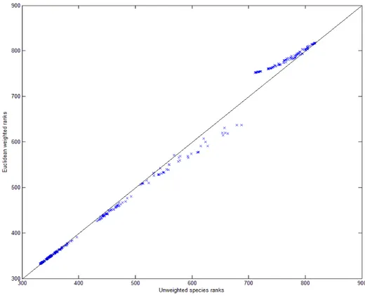
Fig. 2 Euclidean weighted ranks vs. unweighted ranks. The line represents 1:1 agreement
2
Since Tasmania was occasionally in a different cluster from New Zealand, the rankings for Tasmania over all clustering trials
would have been slightly different anyway. However, some clustering algorithms such as Kohonen Self-Organizing Maps
(Kohonen, 1990) are often only run once (Paini et al, 2010). The region weighting technique described here, as demonstrated on
3 Results
Since the ultimate goal of this work is to produce lists of species that threaten geographic regions, species ranks are presented in these results, rather than the absolute risk weighting values. The species ranks resulting
from weighted risks are compared to the original, unweighted ranks in Fig. 2. The gaps in the lower left-hand corner of this plot are caused by groups of species being assigned mean ranks, that is, several species having the same rank. To quantify the difference between the ranks, the species were divided into groups by
inspection and the mean difference between the species in each group found. The results of this are in Table 1.
The weighted ranks for Tasmania are plotted against the weighted ranks for New Zealand in Fig. 3. Since these regions appear in the same cluster, the original, unweighted risk algorithm assigned identical species risk
ranks to both regions. From Fig. 3, however, it is plain that using weighted ranks has produced clearly differentiated risk lists for the two regions, especially with the top-ranked species. The differences between the
two sets of species ranks were again quantified by finding the mean difference between species in each group. The results of this are presented in Table 2.
Fig. 3 Tasmanian species ranks vs. New Zealand species ranks. The line represents 1:1 agreement
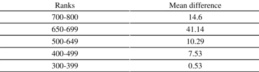
Table 1 Mean difference between groups of weighted and unweighted species ranks
Ranks Mean difference
700-800 14.6
650-699 41.14
500-649 10.29
400-499 7.53
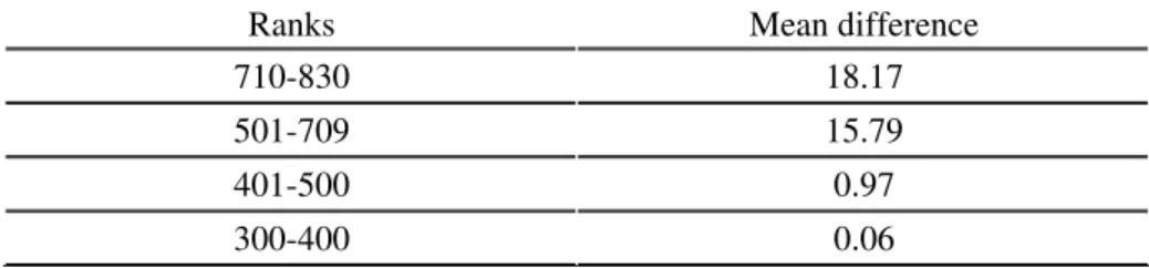
Table 2 Mean difference between groups of New Zealand and Tasmanian species ranks
Ranks Mean difference
710-830 18.17
501-709 15.79
401-500 0.97
300-400 0.06
4 Discussion
Ranks from weighted risks are plotted in Fig. 2. While there is some scattering of the ranks around the middle
region, there is a large upwards shift at the upper-right of the plot. The results in Table 1 show that the largest difference in ranks were between the species in the 650-700 ranked group, where the ranks are the original,
unweighted ranks. This was followed by the species in the 700-844 ranked group. Lower ranked species had their ranks changed much less. This is logical as regions that are more like the target regions will be assigned to the target cluster more often. Weighting by similarity to the target region is therefore acting like a “booster”3
to the risk evaluation process, amplifying the effect of the clustering.
The results of comparing the weighted risks of New Zealand and Tasmania are plotted in Fig. 3. This shows that while there are some very similarly ranked species at the top and bottom ranks, there are many species that
are more highly ranked for Tasmania than they are for New Zealand, and vice versa. The largest difference in ranks was for species ranked 710-844, where the ranks were the original ranks. The mean differences between the lower ranked groups were much smaller. Thus, the weighting method has clearly produced risk ranks that
are specific to the individual regions, despite those regions clustering to the same cluster. It should be borne in mind that only clusters that contained both Tasmania and New Zealand were used to generate these risk ranks.
Therefore, the unweighted ranks were identical for these two regions and the weighted ranks-specific to each region.
Validating the results of this kind of risk analysis is very difficult. Controlled experiments introducing pests into a new environment are of course out of the question. Reports of incursions that have occurred
subsequently to the compilation of the data used in the clustering can be useful, but these reports are sporadic and depend not only upon the detection of the invader but also upon the cooperation of the reporting agency.
Expert opinion of the risks of pests invading tend to be highly subjective or biased (Burgman, 2005), which limits their utility as a comparison. However, some support for this method can be garnered from the example of Chrysomphalus aonidum, which is commonly known as the Florida Red Scale. This pest was in the top twenty of the threat lists in Watts and Worner (2009), and was detected in Auckland, New Zealand, in 2004 (Gill, 2005). It is since believed to have been eradicated by New Zealand biosecurity. Another example is
Ceratitis capitata, the Mediterranean fruit fly. This species was also highly ranked in Watts and Worner
(2009), and is frequently intercepted by New Zealand biosecurity. An established population of C. capitata
was eradicated in 1996 (Gevrey et al, 2006).
Although these techniques were applied to the results of k-means clustering, they could be applied to the outputs of any clustering algorithm. Even if a single clustering run is carried out (such as in Paini et al (2010), where a Kohonen SOM (Kohonen, 1990) was used to perform the clustering), weighting of the neighbour
regions can assist by producing results that are distinct for each region. Weighting factors could also be derived from abiotic factors, such as the similarity of regional climates or even information on trade between
3
regions. Including abiotic factors could improve the accuracy of the risk assessment process and will be the basis of future work.
5 Conclusion
The paper has presented a method of producing highly region-specific species invasion risk rankings from clusters of regional species assemblages. This was achieved by weighting the contribution of each assemblage
within the same cluster as the region of interest.
In a case study re-analysing the previously published results of k-means clustering, weighting the
contributions of assemblages by the Euclidean distance between those assemblages and the target assemblage produced regional risk lists that were clearly differentiated. A comparison of the ranks assigned to species for New Zealand and Tasmania, two regions that were frequently assigned to the same cluster, showed that the
weighting method is capable of producing clearly differentiated risk rankings for individual regions.
Acknowledgements
The authors wish to acknowledge the work of Muriel Gevrey and Joel Pitt who prepared the data used in this research. Data from the Crop Protection Compendium was used with permission of CAB International,
Wallingford, UK.
References
Burgman M. 2005. Risks and decisions for conservation and environmental management. Cambridge University Press, Cambridge, UK
Crop Protection Compendium - Global Module (5th ed). 2003. CAB International, Wallingford, UK
Everitt BS, Landau S, Leese M. 2001. Cluster Analysis, Fourth Edition, Arnold Publishing, London, UK
Gevrey M, Worner S, Kasabov N, et al. 2006. Estimating risk of events using SOM models: A case study on invasive species establishment. Ecological Modelling, 127: 361-372
Gill G. 2005. Spray programme effective against Florida red scale. Biosecurity, 61: 17
Gotelli NJ. 2000. Null model analysis of species co-occurrence patterns. Ecology, 81(9): 2606-2621
Kohonen T. 1990. The self-organizing map. Proceedings of the IEEE, 78(9): 1464-1479
Krebs C. 1999. Ecological Methodology. Addison-Wesley, Longman, NY, USA
Lloyd SP. 1982. Least squares quantization in PCM. IEEE Transactions on Information Theory, 28(2):
129-136
Paini DR, Worne, SP, Cook DC, et al. 2010. Using a self-organizing map to predict invasive species: sensitivity to data errors and a comparison with expert opinion. Journal of Applied Ecology, 47: 290-298
Watts MJ. 2011. Using data clustering as a method of estimating the risk of establishment of bacterial crop
diseases. Computational Ecology and Software, 1(1): 1-13
Watts MJ, Worner SP. 2009. Estimating the risk of insect species invasion: Kohonen self-organising maps versus k-means clustering. Ecological Modelling, 220(6): 821-829
Worner SP, Gevrey M. 2006. Modelling global insect pest species assemblages to determine risk of invasion. Journal of Applied Ecology, 43: 858-867
Zhang WJ. 2010. Computational Ecology: Artificial Neural Networks and Their Applications. World