www.ocean-sci.net/6/997/2010/ doi:10.5194/os-6-997-2010
© Author(s) 2010. CC Attribution 3.0 License.
Ocean Science
Retroflection from a double-slanted coastline:
a model for the Agulhas leakage variability
V. Zharkov1, D. Nof1,2, and W. Weijer3
1Geophysical Fluid Dynamics Institute, Florida State University, Tallahassee, FL, 32306, USA 2Department of Oceanography, Florida State University, Tallahassee, FL, 32306, USA
3New Mexico Consortium, Los Alamos National Laboratory, Los Alamos, NM 87545, USA Received: 26 March 2010 – Published in Ocean Sci. Discuss.: 5 July 2010
Revised: 9 November 2010 – Accepted: 10 November 2010 – Published: 13 December 2010
Abstract. The Agulhas leakage to the South Atlantic ex-hibits a strong anti-correlation with the mass flux of the Agul-has Current. When the AgulAgul-has retroflection is in its normal position near Cape Agulhas, leakage is relatively high and the nearby South African coastal slant (angle of derivation from zonal) is very small and relatively invariant alongshore. During periods of strong incoming flux (low leakage), the retroflection shifts upstream to Port Elizabeth or East Lon-don, where the coastline shape has a “kink”, i.e., the slant changes abruptly from small on the west side, to large (about 55◦) on the east side. Here, we show that the variability of rings shedding and anti-correlation between Agulhas mass flux and leakage to the South Atlantic may be attributed to this kink.
To do so, we develop a nonlinear analytical model for retroflection near a coastline that consists of two sections, a zonal western section and a strongly slanted eastern sec-tion. The principal difference between this and the model of a straight slanted coast (discussed in our earlier papers) is that, here, free purely westward propagation of eddies along the zonal coastline section is allowed. This introduces an in-teresting situation in which strong slant of the coast east of the kink prohibits the formation and shedding of rings, while the almost zonal coastal orientation west of the kink encour-ages shedding. Therefore, the kink “locks” the position of the retroflection, forcing it to occur just downstream of the kink. Rings are necessarily shed from the retroflection area in our kinked model, regardless of the degree of eastern coast slant. In contrast, a no-kink model with a coastline of intermediate slant indicates that shedding is almost completely arrested by that slant.
Correspondence to: D. Nof ([email protected])
We suggest that the observed difference in ring-shedding intensity during times of normal retroflection position and times when the retroflection is shifted eastward is due to the change in the retroflection location with respect to the kink. When the incoming flux detaches from the coast north of the kink, ring transport is small; when the flux detaches south of the kink, transport is large. Simple process-oriented nu-merical simulations are in fair agreement with our analytical results.
1 Introduction
The normal retroflection position of the Agulhas Current (AC) is to the southwest of Cape Agulhas (Lutjeharms and Van Ballegooyen, 1988a). Occasionally, however, the retroflection shifts upstream and occurs near Port Elizabeth or East London (Fig. 1, upper panel). This unusual east-ward shift typically occurs during periods of strong incom-ing flux (SIF). The coastline geometries near the two differ-ent retroflection areas are distinctly differdiffer-ent. During SIF, retroflection occurs near a coastline that is strongly concave (i.e., in plan view, the on-land angle between the two straight coasts is considerably smaller than 180◦), whereas during times of normal position of retroflection (NPR), the nearby coastline is weakly concave.
This article supplements our recent theoretical investiga-tions suggesting that Agulhas ring-shedding variability is pri-marily due to the inertial and momentum imbalances in com-bination with the coastal slant (deviation from zonal orienta-tion) near the retroflection (Zharkov and Nof, 2008a, b: here-after referred to as ZNa, ZNb, and, jointly, ZNab). Here we push our recent work closer to reality by introducing a “kink” in the previously straight coastline configuration.
first six months after release of all floats in 1986− −
flection is consequ
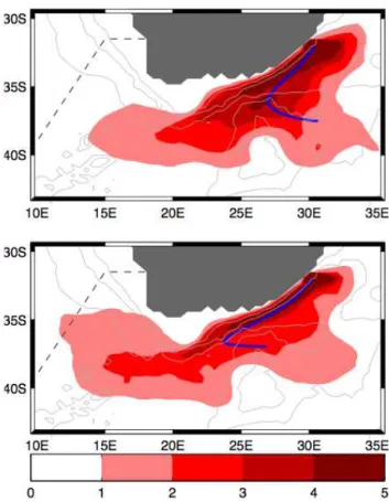
Fig. 1. The transport density (shaded patches, in Sv) based on floats distribution. Upper panel: the first six months after release of all floats in 1986–1987, when the AC transport was 65.4 Sv. Lower panel: the same but for 1988–1989, when the AC transport was 61.0 Sv. The thick blue lines show the transport mean trajecto-ries. Bathymetry is shown by the gray lines (1500 m contour in-terval). The dashed line is the location of the Good Hope line over which the Agulhas leakage is calculated. During the time of lower transport (lower panel), the current detaches from the continental slope farther downstream. The retroflection is consequently moved westward and the magnitude of the Agulhas leakage is increased. Adapted from Van Sebille (2009).
This refinement allows us to mimic more closely the actual coastline orientation. In a (land) concave model the land pro-trudes toward the ocean so that the ocean occupies more than half the 360◦plane. In the convex model, the ocean bulges into the land so that it occupies less than half the 360◦plane. The former case is applicable to the southern tip of Africa, whereas the latter is more appropriate to the southwest At-lantic. Our focus here will be on the South African case. 1.1 Observational background
Although the positions of retroflected currents are in general determined by the position of the zero wind stress curl, the exact path and position of the AC retroflection adjacent to the coastline is sensitive to various parameters such as the AC volume transport and the coastline orientation (see e.g.,
Lut-jeharms and Van Ballegooyen, 1984). During NPR, when the AC volume transport is low, the Agulhas retroflection pro-trudes westward and is located near a coastline of low slant and little curvature. During these times, there is an increase of warm water influx (via rings) into the South Atlantic. During SIF, on the other hand, the retroflection shifts east-ward to a location where the coastline has a concave “kink” (i.e., where the on-land angle between the two approximately straight coastlines is considerably smaller than 180◦). This is probably consistent with the observation that rings in the Ag-ulhas region are typically shed about 5–6 times per year, but the period of their formation increases sometimes to almost half-a-year (e.g., Byrne et al., 1995; Gordon et al., 1987; Lut-jeharms, 2006; Schouten et al., 2000; Van Aken et al., 2003). Interestingly, there is no consensus on the significance of seasonal variability of the retroflection and other Agul-has features and processes. Shannon (1985), and Esper et al. (2004) point to a seasonal variability of the retroflection position, which is in agreement with the numerical calcula-tions of Reason et al. (2003) suggesting that the incoming flux is maximal in winter and minimal in summer. Ffield et al. (1997) also point to seasonal variation in the Agulhas vol-ume transport, and some seasonality in the Agulhas sea sur-face height was also shown by Matano et al. (1998). Goni et al. (1997) suggest that seasonality can very moderately affect ring shedding. Their observations during 1992–1995 sug-gest that six out of the 17 consecutive Agulhas rings were first observed in austral summers while only four rings were first observed in winters. In addition, the volumes of all four winter-rings were less than the value averages over all rings. However, such volume variations are not commonly believed to be responsible for significant seasonal modifications of the rings’ shedding regime (e.g., Van Sebille, 2009).
In contrast to the above ideas of seasonality, Lutjeharms and Van Ballegooyen (1988b), and Lutjeharms (2006) speak about anomalous and more occasional eastward shifts of the Agulhas retroflection area. Associated with these shifts is a decrease in ring shedding.
The anomalous eastward migration of Agulhas retroflec-tion occurs usually 2–3 times per year and lasts 3–6 weeks. There have also been observations of very irregular, inter-annual variations of the retroflection position. For instance, the so-called “early (upstream) retroflection” events occurred in 1986 (Shannon et al., 1990) and in 2000–2001 (Quar-tly and Srokosz, 2002; De Ruijter et al., 2004), when the AC retroflected to the east of the Agulhas Plateau. A de-crease in Agulhas leakage in 1986 (during the first known early retroflection) is clearly seen in Fig. 6 of Van Sebille et al. (2009b). During the second early retroflection event (2000–2001), no eddies were shed for about five months.
in 1986–1987 (upper panel) whereas El-Ni˜no occurred in 1988–1989 (lower panel). We can expect the time periods between consecutive La-Ni˜na events to be comparable to the classic ENSO periods but with no regularity. (Note that in Biastoch et al., 2008, they are two years apart.) In addition, duration of La-Ni˜na events in the Indian Ocean and the AC are much shorter than for the usual La-Ni˜na conditions in the Pacific (see e.g., Van Sebille et al., 2009a, VSa, hereafter). 1.2 Theoretical background
An anti-correlation between the AC transport and the west-ward protrusion of the retroflection (and, therefore, increase in Agulhas leakage) has been pointed out by De Ruijter and Boudra (1985), Boudra and Chassignet (1988), Esper et al. (2004), and VSa. It has also been shown that the posi-tion of Agulhas retroflecposi-tion has a strong impact on the inter-annual variations of the inflow to the South Atlantic, which, in turn, significantly affects the decadal variability in the At-lantic meridional overturning circulation (Weijer et al., 1999, 2002; Biastoch et al., 2008). While all of these studies are informative, none specifically addresses the dynamic balance involved in the anti-correlation modeling.
The idea that coastal geometry is important to retroflecting currents is also not new. It was recognized by Ou and De Ruijter (1986), Boudra and Chassignet (1988), De Ruijter et al. (1999), Chassignet and Boudra (1988), and Pichevin et al. (1999), though none of these earlier studies focused specifically on the issue that we are addressing here, where a small slant allows for stronger eddy production.
Of these earlier studies, Ou and De Ruijter (1986) is the closest to our new kink model. Here the authors assumed that the flow has a scale larger than the Rossby radius and that the flow scale is also larger than the continental radius of curvature. In their model, the AC attempts to follow the coastline but cannot continue to do so when the coastline curves strongly to the right (looking downstream) because the curving is too sharp for the current to mimic. Conse-quently, the current separates from the continent and a space opens up between the two. In its unsuccessful attempt to con-tinue hugging the continent, the current cyclonically loops upon itself in this open space. Supposedly, this looping pro-duces the retroflecting eddies. The main weakness of this theory is that it requires a relatively large coastline curvature for ring production, and so this model cannot be used to trace the dynamics of shedding in areas of only weak curvature. Also, according to this theory, the thermocline outcropping is a necessary condition for detachment of the AC from the coast.
For the case of a nearly zonal coastline and within a 1.5-layer model, Nof and Pichevin (1996) showed that baroclinic rings are generated to compensate for the eastward retroflect-ing current momentum flux (flow-force). ZNa elaborated on this condition and pointed out a “vorticity paradox”: only rings with strong relative vorticity satisfy the equations of
momentum and mass conservation. Mathematically, this means that the ratio, 8, of the mass flux going into eddies to the incoming mass flux is 4α/(1 + 2α), whereαis the eddy intensity coefficient (the eddy’s orbital velocity isα f R/2 whereRis the eddy radius andf is the Coriolis parameter; in the case of zero PV,αis 1). Therefore, the necessary con-dition8≤1 is satisfied only forα≤0.5. This is because, in the strong inertial limit (α >1/2), the momentum flux of the retroflecting current is just too high for rings to compensate for it, no matter how many rings are produced and no matter how large they are. One way to avoid this paradox is to fo-cus on currents retroflecting near coastlines with slants larger than a threshold value (∼15◦).
ZNb considered the case of a single straight coastline and showed that the value of8decreases monotonically to zero as the slant grows from zero to 90◦. A critical coastline slant
was defined, below which there is rings shedding and above which there is almost no shedding. Indeed, in the case of a meridionally directed incident current, no eddy detachment has been found in numerical models (Arruda et al., 2004). 1.3 Present approach
In this paper, we take a step closer to reality by considering a retroflection along a coast with a kink, i.e., a concave or con-vex coast consisting of two straight coastlines with different angles of slant. It can be inferred from Pichevin et al. (2009), as well as from others, that the effect of an abrupt change of slant is significant when the distance between the point of coastal inflection and the point of the AC coastal detachment is within the ring diameter. It will become clear later that this appears to be the case fairly often because the kink locks the position of the retroflection.
We shall consider three separate cases: Concave I, Con-cave II and ConCon-cave III. In ConCon-cave I, the western segment of the coastline is purely zonal. This is a special case has ap-plication to both NPR and SIF conditions; the eastern angle of slant will be smaller for the NPR case. Concaves II and III will be considered as simplifications of the South African coast geometry (Fig. 2), in that the western segment will no longer be constrained to a purely zonal orientation. In Con-cave II, which is meant to approximate the coastline near the retroflection during NPR, the angle between the two (non-zonal) coastlines is almost 180◦ so the degree of concav-ity is weak. In Concave III, which represents the coastline near the retroflection during SIF, the angle is much smaller so the system is sharply concave. We will develop a non-linear retroflection model (Fig. 3) using the slowly varying approach suggested by Nof (2005).
In considering the model geometry, we will neglect the varying offshore bathymetry even though the southern AC is steered by the shelf break rather than the coastline (Lutje-harms, 2006). This simplification is justified because when the retroflection occurs not far from the concavity of the coastline, the shelf break and coastline are parallel. Also,
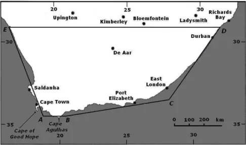
Fig. 2. Map of South Africa with a superimposed pentagon showing the model geometries. ABC corresponds to Concave II (coastline representation for NPR), and BCD corresponds to Concave III (SIF). Concave I is a zonal south-facing coastline contiguous with a slanted eastern shore (that could be NPR or SIF represented by different angles of slant or a mean slant).
rings shed from the eastward-shifted retroflection propagate westward and avoid the southern part of the Agulhas Bank because its scale is smaller than the scale of one separated eddy.
There are two important differences between the kink and the no-kink models. First, in the kink model, rings can escape from the generation area faster than in the no-kink model because in the no-kink model the rings are forced into the slanted wall. By contrast, in the kinked model, the rings are almost completely free to propagate westward. This implies that more rings will be generated in the kinked model be-cause they can quickly escape a recapture by the new rings generated behind them. Second, the momentum flux in the direction corresponding to the rings’ migration route (al-most zonal) is smaller in the kinked model than in the no-kink model because this flux corresponds to merely a com-ponent (cosγ) of the upstream longshore momentum. This implies fewer and smaller eddies in the kinked-model case. These two processes above compete, with the first encourag-ing and the second inhibitencourag-ing rencourag-ing production in the kinked model. Which one dominates depends on the particular cir-cumstances. In the cases that we considered, the first process dominates, i.e., there are considerably more rings produced in the kinked model case.
This paper is not self-contained. Readers interested in fur-ther details may consult ZNab. In Sect. 2, we introduce the governing equations that control the development of the base eddy on a kinked coastline. In Sect. 3, we present model solutions for cases of varied parametersαandγ. Section 4 is devoted to an examination of ring size, drift speed, and shedding period. In Sect. 5, we give the results of numerical simulations and compare them with the analytics. Section 6
is devoted to an application of our results to the variability in Agulhas ring shedding and leakage into the South Atlantic via rings. Finally, we summarize and discuss our results in Sect. 7.
2 Statement of problem
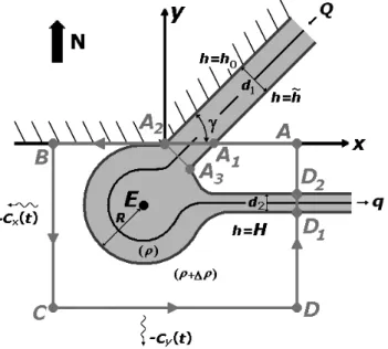
As in ZNab, we consider a boundary current (with densityρ) embedded in an infinitely deep, stagnant lower layer (whose density isρ+1ρ), except that here the vertical boundary on the west is not a single straight line. The first coastline to be considered (Concave I) consists of two rectilinear sections (Fig. 3): one is zonal, and the second one is slanted at an angleγ that varies between 0◦ and 90◦. The current flows southwestward along the slanted section and then retroflects south of the kink.
γ =0 °
β
− − β
Fig. 3. Schematic diagram of the Concave I case: a zonal west-ern shoreline segment with a slanted coastline (γ=0 to 90◦) to the east. The hatch marks indicate land. Eis the center of the base eddy. The incoming fluxQflows along the wall, and the outgo-ing (retroflected) fluxqis directed to the east. The widths of the currents ared1andd2, respectively. The “wiggly” arrows indicate the migration of the base eddy; this migration results from both the eddy growth, which forces the eddy away from the zonal wall, and fromβ, which forces the eddy along this wall. The migration ve-locity component−Cy(t )is primarily due to eddy growth, whereas −Cx(t )is primarily due toβ. The thick grey line (with arrows)
indi-cates the integration path, ABCDA; ˜h is the upper layer thickness of the stagnant region wedged between the upstream and retroflecting currents, andH is the off-shore thickness. The ring forms down-stream ofA2and immediately starts migrating westward. Conse-quently, the integrated momentum flux along the slanted wall in-volves an unknown force acting on the wall (and therefore cannot be used) but the zonal integrated momentum does not.
Ras a function of timet,
(αf0)3 240
h
2(1+cosγ )R5−5(δ12−δ22)R3−5(δ13cosγ+δ23) R2+(3δ51cosγ+5δ12δ32−2δ25)i+α
2f 0g′h0 12
h
(1+cosγ )R3−(δ31cosγ+δ32)i−π R2
"
g′H+α(2−α)f 2 0R2 16
#
dR
dt =0. (1)
This equation differs from its counterpart in ZNa in that Eq. (1) the ZNa terms withαβR2are absent here, and Eq. (2) in ZNa cosγ serves as a multiplier for other terms than here in Eq. (1). The remaining equations defining the functions
R(t )and8(t )are the same as in ZNa and are not reproduced here.
3 Solution
We solved the system of equations, again by using the Runge-Kutta method of the fourth order. We used: Q= 70 Sv;g′=2×10⁻²ms−2;f=8.8×10⁻⁵s−1 (correspond-ing to 35◦ of latitude) and, we considered two cases of
h0:0 m and 300 m. The parameterαwas varied between 0.1 and 1.0, andγwas varied between 0◦and 90◦. The functions
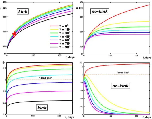
R(t )and8(t )for the case of zero PV (α=1),h0=300 m, andβ=2.3×10⁻¹¹m−1s−1 are shown in Fig. 4 (left pan-els). For a comparison, analogous plots (without triangles and squares) for the ZNa, ZNb model are also shown (right panels). The quantitative difference between the two models is obvious. Only the curves forγ=0◦are identical because the case of a zonal wall is the same in both models. In the kinked case, theRvalues grow infinitely witht, and the8(t )
curves approach asymptotic values that decrease with grow-ingγ. As expected, in the case of a zonal wall (γ=0◦), the
asymptotic value is close to 4/3. All the curves forγ <60◦ intersect the “dead line”8=1, indicating that the “vortic-ity paradox” occurs at the sections of curves above this line. We can see that the paradox could be circumvented only for
γ≥60◦(instead ofγ≥15◦as in the ZNa model), because it is for this minimal value ofγ that 8 does not intersect the deadline. The asymptotic value forγ=90◦ is close to 2/3, indicating that this case is similar to the ballooning-of-outflows problem (Nof and Pichevin, 2001).
For smaller values ofα(vorticity coefficient), the curves ofR(t )and8(t )(not shown) are similar to those shown in Fig. 4, but the asymptotical values of8go down with de-creasingα. As expected from the analytical model, these val-ues can indeed be approximated by 2α(1+cosγ )/(1+2α). This result implies that the detached rings compensate for the momentum of both the entire retroflected current and the zonal projection of the incoming current. Therefore, the “vorticity paradox” is circumvented when the slant of the tilted coastline section is not less than cos−1(1/2α), which is 60◦for zero PV (α=1).
4 Detachment of rings
4.1 Lower and upper boundaries for final eddy size Following ZNb, the generation period for each individual ring is,
tf=(2Rf+d)/|Cxf|, (2) whered is the distance between two consecutive rings, Cx is the ring propagation rate in the zonal direction, and the subscriptf denotes the final value (i.e., the value at the time of detachment). The lower boundary for the final eddy size (Rf l) is obtained from the condition of “kissing eddies”, i.e.,
d=0.
Φ
γ
γ
γ
=0 Φ =1
β
= × − − −α
=1 =
Fig. 4. Base eddy radiusR(upper panels) and mass flux ratio8(lower panels) as functions of time for different values ofγ: Concave I case (left) and analogous no-kink ZNa model (right). For the kink model,γindicates the angle of the eastern shoreline segment; for the no-kink modelγ indicates the angle of single-segment slant. The straight dotted “dead lines” (lower left panels) show the limit ofq=0,8=1. Red triangles and squares (upper left) denote the lower and upper boundaries of the detachment period forβ=2.3×10⁻¹¹m−1s−1,α=1, h0=300 m.
Next, we define the upper boundary (Rf u) for the basic eddy’s final size, and for the generation period (tf u). This expression implies that the ring can propagate at least its own diameter:
tf u
Z
0
|Cx|dt=2Rf u. (3)
Physically, the upper boundary corresponds more directly to the detachment of isolated rings, whereas the lower boundary is a condition for the eddy chain formation. So, rings detach and propagate out of the retroflection area only whenRf lis indeed less thanRf u.
4.2 Analysis of lower and upper boundaries
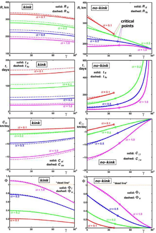
Here, we shall use 2.3×10⁻¹¹m−1s−1 and 6×10⁻¹¹m−1 s−1forβ. The first is a commonly used value, whereas the second is magnified (more convenient for the model runs). The left upper panel of Fig. 5 showsRf l andRf uas func-tions ofγ, and the right upper panel shows the analogous no-kink results. For both models, the functions decrease as
γ grows. In the kink (Concave I) case, the curves of Rf l andRf u do not intersect, implying that there is no critical
slant angle. The difference between the lower and upper size boundaries decreases slightly with diminishingα. In the con-trast, in the ZNb no-kink model, the lower and upper bound-aries do intersect: the critical points of intersection are cir-cled. (When the slant is supercritical, rings do not move out of the retroflection area fast enough and, consequently, they are recaptured by the flow behind.) In addition, in the ZNb model, the curves forα=1 terminate at a value ofγ that is significantly less than 90◦because for largeγ and smallα, the base eddy is forced into the wall and is not allowed to grow. Such a process does not occur in the Concave I model considered here.
The ring detachment period tf (Fig. 5, second row) de-creases with growingα, as does the final eddy radius (first row). Here in the kink case, we again see no intersection or convergence of the curves depicting upper and lower bound-aries (i.e., no critical angle). Eddy speed decreases with in-creasingα(Fig. 5, third row). Another difference between the kink model and the ZNb model is that the no-kink tf l andtf u tend to infinity and Cξ l and Cξ u go to zero when
Φ
Φ
γ
ξ ξ
=
β
=
×
− − −
Fig. 5. Final base eddy radii (Rf landRf u), ring generation periods (tf l andtf u), ring zonal propagation rates (CxlandCxu), and mass
flux ratios (8land8u) as functions ofγfor Concave I (left panels) and analogous ZNb model parameters (right panels, with non-zonal ring
propagation ratesCξlandCξu), forh0=300 m andβ=2.3×10⁻¹¹m−1s−1. The curves are paired, where solid and dashed lines show the lower and upper boundaries of the eddy radius, respectively. In the Concave I case, upper and lower boundaries do not intersect. In the ZNb model, upper and lower boundaries do intersect, implying the existence of critical slant angles. Such critical points are circled.
4.3 Mass flux going into rings
We will now estimate8, the ratio of mass flux going into the growth of the rings to the incoming flux. Because8depends on time, this ratio is obtained by averaging instantaneous val-ues over the period of eddy generation. As expected, av-eraged values of8for both models decrease with increasing coastline slantγ(Fig. 5, lower panels). In the kink model, the
8uand8lcurves for a givenαdo not intersect. In contrast, in the analogous ZNb case, the8curves intersect twice, first at points corresponding toγ between 4◦and 35◦, and then again at higherγ when the angle is critical (andα >0.1); Fig. 5, lower right panel). For both models, low-angle values of8fall above the “dead line” (i.e., appearance of the “vor-ticity paradox”) forα >0.8. Maximum time-averaged8 val-ues, which occur whenα=1, are considerably less than 4/3, because the instantaneous values of8are much less than 1 at the beginning of eddy development. Forγ >34◦, all the curves are below the dead line. Distinguished8 characteris-tics for Concave I are as mentioned above: no critical angles, and8does not tend to zero with growingγ.
One can show that varying upper layer thickness has only a very weak influence on the detached rings (results not shown). Using the modified value of β rather than the standard value does not lead to qualitative differences ei-ther. However, the propagation rate of rings increases, and the generation period decreases. Also, the lower and upper boundaries become close to each other for largeγ, meaning that the shedding regime is nearly critical but not supercriti-cal.
5 Numerical simulations: Concave I
As in our previous studies, we used a modified version of the Bleck and Boudra (1986) reduced gravity isopycnic model with a passive lower layer and the Orlanski (1976) second-order radiation conditions for the open boundary. The basin size was taken to be 3200×1600 km2. The continent (Figs. 6 and 7) was modeled by a fixed meridional western wall (600 km long), a southern wall that could be either 2200 km (in the caseγ=0◦) or 1000–1200 km long, and, forγ >0◦, an eastern wall inclined by the angleγ to the zonal direction (γ varied between 15◦and 90◦in steps of 15◦). The walls were taken to be slippery.
The experiment began by turning on an outflow att=0; the numerical source was an open channel containing stream-lines parallel to the slanted wall in the incoming current and horizontal in the outgoing flow. The initial velocity profile across the channel was linear, and the thickness profile was parabolic. Because each run provides many data points, it is believed that we have enough data to work with. We chose the initial PV of outflows such that the starting values ofα
were 0.1, 0.4, and 1.0. As expected, at the beginning of each run when the orbital velocities were still high,αchanged rel-atively quickly.
The numerical parameters were: (i) a time step of 120 s; (ii) a grid step of 20 km; (iii) a Laplacian viscosity coefficient ofν=700 m2s−1forγ >15◦and forγ=15◦,α >0.1; and
1000 m2s−2 forγ =15◦, α=0.1. Other parameters were
g′=2×10⁻²ms−2, f0=8.8×10⁻⁵s−1, Q=70 Sv, β= 2.3×10⁻¹¹m−1s−1 (realistic) or 6×10⁻¹¹m−1s−1 (mag-nified), and the initial value ofh0=0 or 300 m. We ran all the experiments for a long time (about 210 days for most, but about 700 days for some), so that even the zero PV ex-periment ultimately had its PV strongly altered by the cumu-lative effects of friction. Therefore, we used time-averaged values ofαin our quantitative comparisons. For most of the experiments, we chose the magnified value ofβwhich accel-erates ring detachment and makes our runs more economical. For the realistic value ofβ, the model results do not qualita-tively differ from those obtained with the magnifiedβ, but the time required for the numerical runs does noticeably in-crease. In addition, for largerβ, the effect of viscosity gets even stronger, which makes the view of some rings extremely fuzzy. Finally, increasingβ increases the ring propagation rate, compensating for the deceleration by viscosity.
Viscosity values used in these experiments may be con-sidered high for studying an essentially inertial process like Agulhas ring shedding; however these values are essential to maintain numerical stability for the required duration of the experiments. Still, the relatively coarse resolution used in these experiments (∼20 km) assures clear dominance of inertial forces over viscous friction.
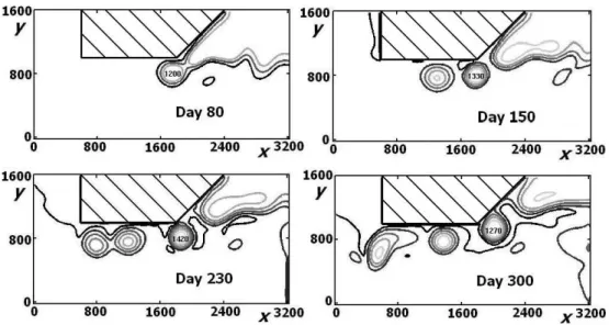
We examine first some general simulations not meant to represent NPR or SIF but to illustrate model dynamics at a fixed outflow latitude. For most Concave I cases, our nu-merical simulations (withγ=15◦, 30◦, and 45◦) show the
detachment of two or three rings from the retroflection area during the first 200 days (Fig. 6). As a secondary effect, the second eddy often collided with the first one. A similar ef-fect was present in the numerical simulations of Pichevin et al. (1999), though the authors of that paper did not note it. Our simulations withγ=60◦showed increased influence of some rings formed in the upstream flow (due to meandering, not retroflection). Such rings moved westward and reached the retroflection area but, upon approaching the developing base eddy, were weakened and did not affect it.
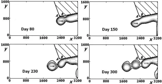
The simulations with γ=75◦ and 90◦ confirm our con-jecture that these angles are “almost critical” for modifiedβ. Indeed, the runs withα=0.1 were very similar to those for
γ=60◦, i.e., there was a detachment of two eddies during
the first 200 days. However, a more typical situation is dis-played in Fig. 7 (γ=75◦). During 300 days of simulation,
γ
γ
=α
=1 =ν
= 0 −β
= × − − −Fig. 6. Upper layer thicknesses for the case of a Concave I coastline with a modest kink (midsizeγ) and a current with high upstream vorticity (γ=45◦,α=1,h0=300 m,ν=700 m2s−1, andβ=6×10⁻¹¹m−1s−1). The eastern wall is not critically slanted, so rings are formed upstream of the kink. Thicknesses are given in meters, and the x and y scales are in kilometers. This figure, as well as Fig. 7, is given here merely to illustrate the dynamics – both figures are not necessarily associated with either the SIF or NPR, whose numerical runs are displayed in Figs. 9 and 10.
γ
γ
=α
= .4 =ν
= 0 −β
= × − − −Fig. 7. Upper layer thicknesses for the case of a Concave I coastline with a sharp kink (largeγ) and a current with modest vorticity (γ=75◦, α=0.4,h0=300 m,ν=700 m2s−1, andβ=6×10⁻¹¹m−1s−1). Here, the eastern wall slant is too high to allow for ring production, so rings are produced just downstream of the kink, which effectively locks the position of the retroflection. Only one eddy is detached; a second one is about to be detached on day 300.
then propagate into the retroflection area, forcing the base eddy to detach as well (not shown).
If rings shedding were completely prevented by re-capturing (such as in the super-critical case of the retroflec-tion from a straightforward no-kink slanted coast), then we would not be able to say how, and if, the retroflec-tion paradox (Nof and Pichevin, 1996) could be circum-vented. It is worth mentioning here in passing that Pichevin
et al. (1999) suggest that according to their simulations, upstream rings that formed off-shore (in the northeastern part of the retroflected current) detached and ultimately re-encountered the approaching current. They supposed that these events were artificial, suggesting that, in nature, such eddies are observed to be advected eastward. However, Lut-jeharms (2006, p. 227) notes that at least cold cyclonic eddies (formed in the Agulhas Return Current) propagate westward
γ
α =
=
α
= =
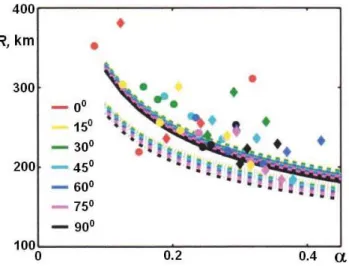
Fig. 8. Ring radii from the analytical kink model and corresponding numerical simulations for a range of eastern wall slants (γ). The slant of the western segment is nearly zero. Modeled values ofRf l
andRf u are plotted againstαforh0=0 (solid and dashed lines, respectively) and forh0=300 m (dash-and-dotted and dotted lines, respectively). The numerical values ofR correspond toαbeing, as in ZNb, averaged over the periods of simulations (diamonds for h0=0 and circles forh0=300 m). The numerical radii are larger than in our model because of viscosity, which spins the rings down flattening them out.
and are subsequently absorbed by the first meander encoun-tered in their westward paths.
We also quantitatively compared analytical and numerical model results for the case of a Concave I kinked coastline. The outcomes are similar to those mentioned in ZNb, i.e., the agreement in rings radii is good, with possible differences of about 20%, on average (Fig. 8). However, propagation rates in the numerics are on average about half those in our analytical model, again because of the effect of viscosity.
6 Agulhas rings leakage variability
Our purpose here is not to duplicate nature point-by-point (for which a more sophisticated model subject to much longer runs is needed) but rather to point out the dynam-ical importance of a sudden change in the coastline slant (i.e., a kink). No-kink model simulations with a moder-ate coastline typical of meant SIF conditions (35–40◦), lead
to a sub-critical shedding regime forα >0.15 but a criti-cal or super-criticriti-cal regime for the more realistic values of
α≤0.15 (Fig. 5). Therefore, the applicability of this no-kink model to real ocean conditions is poor. Moreover, the curves forα=0.1 terminate atγ=35◦, implying that the no-kink model is invalid in such conditions because according to this model, the base eddy cannot grow in the retroflection area. Hence, we suggest that our Concave I model describes the behavior of the Agulhas retroflection better than does the
no-Table 1. Theoretically estimated (Concave I) shedding ratios as a function of the vorticity coefficient,α.
α 0.1 0.2 0.4 0.6 0.8 1.0
Eddyradius for SIF
Eddyradius for NPR 0.96 0.96 0.96 0.96 0.96 0.96 Sheddingperiod for SIF
Sheddingperiod for NPR 1.04 1.05 1.06 1.06 1.06 1.06 Eddyvelocity for SIF
Eddyvelocity for NPR 0.93 0.92 0.91 0.91 0.91 0.90
kink model, and (Fig. 2) we takeγ=15◦as representative of NPR conditions andγ=60◦for SIF.
Using the analytical Concave I model, we estimated SIF:NPR ratios of various shedding parameters (Table 1). All the numbers here are obtained by numerical realization of our Eqs. (2) and (3), with an error of 0.1% or less. It is seen that the intensity of ring shedding significantly de-creases during SIF – i.e., eddies are produced less frequently and their velocities are lower than during NPR. Therefore, the mass transport from the Indian Ocean to the South At-lantic is weaker during SIF than during NPR (despite the non-critical regime in both cases). Note that the parameter ratios given in Table 1 are almost independent ofα.
To fit the model geometry to nature and make the horizon-tal scales as close as possible to their real values (Fig. 2), we adopted Concave II as representative for NPR conditions and Concave III for SIF. The SIF shedding regime near the kink (point C in Fig. 2) is shown in Fig. 9 for weak vorticity and shallow depth. The NPR shedding regime with the retroflec-tion near point B is shown in Fig. 10. The retroflecretroflec-tion lat-itude here is south of that for the Concave III case. Note that we moved here the strongly slanted easternmost shore-line segment out of the calculation frame. (Otherwise, the area of the numerically simulated retroflection shifts gradu-ally to the east, as would occur during a restoration of the SIF regime.) Also, to maintain numerical stability, we had to increase the viscosity here by about 20% over that in the Con-cave III case. The eddy generation period for this NPR sim-ulation is less than that for SIF (Fig. 9) because, although the first two eddies are generated almost at the same time in both cases, the third one lags noticeably in the SIF case. Also, the rings’ radii are greater under NPR conditions (Fig. 10), im-plying that the leakage during NPR is larger than during SIF. The shed NPR eddies form a chain, mainly in the open ocean. The results are not altered appreciably for simulations with stronger vorticity and greater upper layer thickness. We note also that the Concave II and Concave III numerical simula-tions with closely spaced rings require higher viscosity for stability than that in Concave I simulations (Figs. 6 and 7) because of higher shear.
α
= .4 =ν
= 0 −β
= × − − −Fig. 9. Upper layer thicknesses for the case of a Concave III coastline and a modest vorticity current that retroflects near the kink (α=0.4, h0=0,ν=1000 m2s−1, andβ=6×10⁻¹¹m−1s−1). This case is representative of SIF times, when the Agulhas retroflection is shifted eastward.
α
= .4 =ν
= 0 −β
= × − − −Fig. 10. Upper layer thicknesses for the case of a Concave II shoreline and a modest vorticity current that retroflects near the western termination of the slightly slanted coastline (α=0.4,h0=0,ν=1000 m2s−1, andβ=6×10⁻¹¹m−1s−1). This case is representative of NPR times. The strongly slanted section is moved out of the figure. Rings generation occurs more often than in Fig. 9, and the rings’ radii are larger.
an initialαof 1.0, we obtained a mean generation period of 123 days for SIF (with a standard deviation, SD, of 40.2 d) and 93 d for NPR (with SD of 20.5 d). The SIF:NPR ratio is therefore 1.32 (SD is 0.36), which is greater than the theoret-ical value of 1.06 (Table 1). Forα of 0.4, the averaged SIF and NPR shedding periods were 118 d (with SD of 43.9 d) and 110 d (with SD of 18.1 d), respectively. The SIF:NPR ratio is then 1.07 (SD is 0.31), which is very close to the theoretical value. In our simulations forαof 0.1, the eddy very quickly collapsed due to the relatively greater impor-tance of viscosity, and the estimates of average generation
period have large relative errors (60%). The obtained values were 120 d for SIF (with SD 71.9 d) and 145 d for NPR (with SD 75.3 d), so the ratio is 0.83 (SD is 0.47). It should be noted, however, that the variability in the average period was caused by viscosity rather than by the different initializations ofα. This is because during numerical runs, the eddies’ PV was strongly altered by viscosity, so that the averaged values ofαwere about 0.20–0.25 for all the simulations.
Averaged eddy radii shown were about 180 km for SIF and 220 km for NPR (Figs. 9 and 10), so SIF:NPR ratio is 0.82, which is somewhat smaller than the theoretical value of
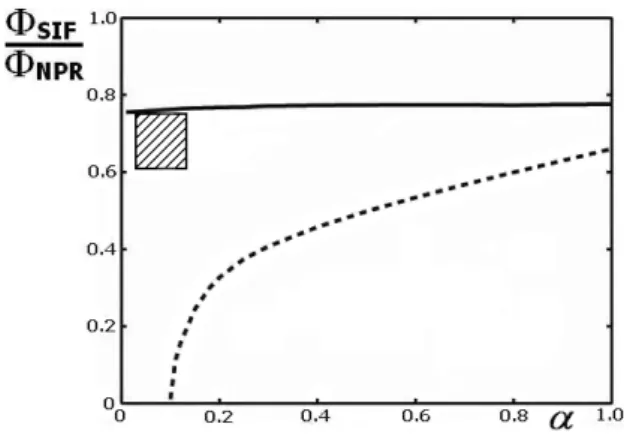
Φ : Φ
° ° °
Fig. 11. Mass transports ratio8SIF:8NPR computed analytically using the kink model (solid line) and ZNb no-kink model (dashed line). The no-kink coastline has a slant of 37.5◦, the average of 60◦ (SIF) and 15◦(NPR). The hatched rectangle shows the confidence area of the observational data from VSa.
0.96 (Table 1). This difference is probably again an effect of viscosity because the thickness of large NPR rings (Fig. 10) is not greater than those of the SIF rings (Fig. 9). Therefore, the ratio of the volume fluxes is expected to be comparable to our theoretical value of 0.77 (solid curve in Fig. 11). Overall, the numerical simulations confirm, at least fairly well, the re-sults of our theoretical modeling. Also, the mean radii and shedding periods for our numerical SIF eddies are close to those in animation created by the GFDL Oceans and Climate group (see http://www.gfdl.noaa.gov/oceans-and-climate): 8 rings shed during 995 days, the averaged value of radius is about 205 km.
We can also compare the ratio of the modeled volume fluxes8with observational data if we assume that the ratio of mass transport carried to the South Atlantic by rings does not differ too greatly from the ratio of the entire Agulhas leakage. According to VSa (their Fig. 1), the average ratio of Agul-has leakage to AC transport (TAL/TAC) is (19.2/60.5)=0.317 when the retroflection is protruded westward (NPR) and
TAL/TAC=(14.2/67)=0.212 when the retroflection is pro-truded eastward (SIF). The SIF:NPR (ratio of these ratios) is 0.67 (confidence range is approximately between 0.61 and 0.75), which is somewhat less than our predicted value of
8SIF:8NPR=0.77 (Fig. 11). This could be due to greater dissipation occurring during the rings’ longer journey from the eastern retroflection area (SIF) to the South Atlantic than from the western area (NPR). Note that the ZNb model with
γ=60◦for SIF (andγ=15◦for NPR) would lead to much
worse results: the considered ratio would change from about 0.4–0.6 for α=1 to zero forα of less than 0.2 (which is closer to real conditions). Using the model results from Fig. 5 (bottom panels) and taking into account that rings carry usu-ally 30–45% of the entire leakage (Doglioli et al., 2006; Van Sebille et al., 2010), we conclude that for the observations of VSa, αwas between 0.03 and 0.13. Even for an aver-age value of the coastal slant (say,γ=37.5◦), the agreement
of no-kink model results with observational data for natural values ofαis poor (Fig. 11). In this figure, we plotted the
8SIF:8NPR versusα for the kink and no-kink (ZNb) mod-els, as well as the confidence region for the data from VSa. It is seen that the curve for the kink model almost touches the confidence area, whereas the no-kink curve goes to zero. (The range ofαwhere the8SIF:8NPRis zero corresponds to the super-critical case where the leakage is shut down).
Finally, using a8SIF:8NPRof 0.77 (Fig. 11) and keeping in mind that the ratio of incoming fluxes for SIF and NPR is 1.10–1.15 (VSa), we conclude that the ratio of outflows is about 0.85–0.90, implying that the kinked coastline plays a defining role in the anti-correlation between the incoming Agulhas flux and the outgoing leakage to the South Atlantic.
7 Summary and conclusions
Using both analytical and numerical models, we showed that the South African coastline geometry exerts a fundamental control on the production of Agulhas eddies and, therefore, the leakage into the South Atlantic. Namely, the coastal kink acts like a valve for the leak. In contrast to what our intuition suggests – that strong flows will be associated with strong leaks – the analytical model with kink implies that smaller leaks occur during times of strong incoming flux (SIF).
We also showed that, for the SIF periods, the kink model gives significantly better results than the straight-coast model in the sense that the difference between the predicted eddy mass flux and the observations is 3–4 times smaller. For NPR, the difference between the concave model and the straight coastline model is insignificant because the angle be-tween the two coastal segments in this case is very close to 180◦. The main aspect of the kink model is that east of the kink the coastline slant is too high to allow for production of rings whereas the slant on the west allows rings production. As a result, the production of rings is allowed in a manner that is quite different from that implied by the mean slant. More importantly, the kink locks the position of the retroflec-tion to just downstream of the kink.
To bring our calculations still closer to reality, we also con-ducted numerical simulations of Concave II and Concave III cases, where the coastline geometry more satisfactorily fits the actual geography near the NPR and SIF positions of the retroflected current (Fig. 2). The Concave II case is taken to be representative of NPR times, and the Concave III case is taken to be representative of SIF. We see (Figs. 9 and 10) that the intensity of eddy shedding decreases during SIF relative to NPR. Therefore, the mass flux going into rings notice-ably weakens during SIF, which is in qualitative agreement with our theoretical results (Fig. 11). Both the theoretical and numerical results indicate that when the Agulhas retroflec-tion protrudes eastward, the ratio8SIFdecreases sufficiently strongly (to about 0.778NPR) to explain the observed anti-correlation between the incoming flux and the outgoing leak-age to the South Atlantic. Indeed, the observed ratio of in-coming fluxes for SIF and NPR is 1.10–1.15; therefore, the ratio of outflows is about 0.85–0.90. On the whole, a compar-ison of our results with VSa (Fig. 11) suggests that our model is consistent with the observed anti-correlation between the AC transport and the Agulhas leakage. Using the earlier ZNb model instead of the new kink model presented here would lead to significantly worse results for leakage via eddies be-cause even the averaged value of the slant near the point of retroflection becomes super-critical (Fig. 11).
The analytical kink model is successfully applied to the case of a weak La-Ni˜na (1986–1987): the error in fitting the observations of mass flux going into eddies is on average 3–4 times less than in the no-kink model simulations. However, it is possible that, as noted by Van Sebille (2009), the no-kink model could be better applied to the strong La-Ni˜na events like the early Agulhas retroflection observed in 2000–2001 (see also, De Ruijter et al., 2004) when eddies shedding was nearly shut down during this period. One possible expla-nation for better applicability of the no-kink model is that during this early retroflection event, the AC was strongly in-teracting with dipoles in the Mozambique Basin. This could result in an AC detachment in the area where the coastline slant does not (yet) change significantly. In view of Pichevin et al. (2009), we expect the no-kink model to be preferable when the AC detaches from the coast somewhere in between East London and Durban, where the coastline is relatively straight. We leave these questions, however, for future inves-tigations.
Acknowledgements. The study was supported by NASA Doctoral Fellowship Grant NNG05GP65H; LANL/IGPP Grant (1815); NSF (OCE-0752225, OCE-9911342, OCE-0545204, OCE-0241036), BSF (2006296), and NASA (NNX07AL97G). V. Zharkov was also funded by the Jim and Shelia O’Brien Graduate Fellowship. We are grateful to Steve Van Gorder for helping in the numerical simu-lations. We also thank Donna Samaan for helping in preparation of the manuscript and Tonya Clayton for assistance in improving the style.
Edited by: E. J. M. Delhez
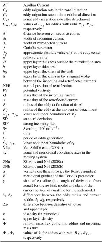
Table A1. List of symbols.
AC Agulhas Current
Cx eddy migration rate in the zonal direction Cy eddy migration rate in the meridional direction Cxf zonal eddy migration rate after detachment Cxl,Cxu values ofCxf for eddies with radiiRf l,Rf u,
respectively
d distance between consecutive eddies d1 width of incoming current
d2 width of retroflected current
f Coriolis parameter
f0 approximate absolute value offat the eddy center g′ reduced gravity
H upper layer thickness outside the retroflection area h upper layer thickness
h0 upper layer thickness at the wall
˜h upper layer thickness in the stagnant wedge between the incoming and retroflected currents NPR normal position of retroflection
PV potential vorticity
Q mass flux of the incoming current q mass flux of the retroflected current R radius of the eddy (a function of time)
Rf radius of the eddy at the moment of detachment Rf l,Rf u lower and upper boundaries ofRf
SD standard deviation SIF strong incoming flux Sv Sverdrup (106m3s−1)
t time
tf period of eddy generation tf l,tf u lower and upper boundaries oftf
VSa Van Sebille et al. (2009b)
x,y zonal and meridional coordinate axes in the moving system
ZNa Zharkov and Nof (2008a) ZNb Zharkov and Nof (2008b)
α vorticity coefficient (twice the Rossby number) β meridional gradient of the Coriolis parameter γ slant of coastline (i.e., angle of derivation from
zonal) for the no-kink model and slant of the eastern section of coastline for the kink model δ1,δ2 differences between the eddy radius and current
widthsd1,d2, respectively
1ρ difference between densities of lower and upper layer
ν viscosity (in numerics) ρ upper layer density
8 ratio of mass flux going into eddies and incoming mass flux
81,8u values of8for eddies with radiiRf l,Rf u,
respectively
References
Arruda, W. Z., Nof, D., and O’Brien, J. J.: Does the Ulleung eddy owe its existence toβ and nonlinearities?, Deep-Sea Res., 51, 2073–2090, 2004.
Biastoch, A., B¨oning, C. W., and Lutjeharms, J. R. E.: Agulhas leakage dynamics affects decadal variability in Atlantic overturn-ing circulation, Nature, 456, 489–492, 2008.
Bleck, R. and Boudra, D.: Wind-driven spin-up in eddy-resolving ocean models formulated in isopycnic and isobaric coordinates, J. Geophys. Res., 91, 7611–7621, 1986.
Boudra, D. B. and Chassignet, E. P.: Dynamics of the Agulhas retroflection and ring formation in a numerical model, I. The vor-ticity balance, J. Phys. Oceanogr., 18, 280–303, 1988.
Byrne, A. D., Gordon, A. L., and Haxby, W. F.: Agulhas eddies: A synoptic view using Geosat ERM data, J. Phys. Oceanogr., 25, 902–917, 1995.
Chassignet, E. P. and Boudra, D. B.: Dynamics of the Agulhas retroflection and ring formation in a numerical model, II. En-ergetics and ring formation, J. Phys. Oceanogr., 18, 304–319, 1988.
De Ruijter, W. P. M.: Asymptotic analysis of the Agulhas and Brazil Current systems, J. Phys. Oceanogr., 12, 361–373, 1982. De Ruijter, W. P. M. and Boudra, D. B.: The wind-driven circulation
in the South Atlantic – Indian Ocean, I. Numerical experiments in a one-layer model, Deep-Sea Res., 32, 557–574, 1985. De Ruijter, W. P. M., Biastoch, A., Drijfhout, S. S., Lutjeharms, J.
R. E., Matano, R. P., Pichevin, T., Van Leeuwen, P. J., and Weijer, W.: Indian Atlantic interocean exchange: Dynamics, estimation and impact, J. Geophys. Res., 104, 20885–20910, 1999. De Ruijter, W. P. M., Van Aken, H. M., Beier, E. J., Lutjeharms, J.
R. E., Matano, R. P., and Schouten, M. W.: Eddies and dipoles around South Madagascar: formation, pathways and large-scale impact, Deep-Sea Res., 51, 383–400, 2004.
Doglioli, A. M., Veneziani, M., Blanke, B., Speich, S., and Grifta, A.: A Lagrangian analysis of the Indian Atlantic interocean ex-change in a regional model, Geophys. Res. Lett., 33, L14611, doi:10.1029/2006GL026498, 2006.
Esper, O., Versteegh, G. J. M., Zonneveld, K. A. F., and Willems, H.: A palynological reconstruction of the Agulhas Retroflec-tion (South Atlantic Ocean) during the Late Quaternary, Global Planet. Change, 41, 31–62, 2004.
Ffield, A., Toole, J., and Wilson, D.: Seasonal circulation in the South Indian Ocean, Geophys. Res. Lett., 24, 2773–2776, 1997. Goni, G. J., Garzoli, S. L. Roubicek, A. J., Olson, D. B., and Brown, O. B.: Agulhas ring dynamics from TOPEX/POSEIDON satel-lite altimeter data, J. Mar. Res., 55, 861–883, 1997.
Gordon, A. L., Lutjeharms, J. R. E., and Gr¨undlingh, M. L.: Strat-ification and circulation at the Agulhas Retroflection, Deep-Sea Res., 34, 565–599, 1987.
Lutjeharms, J. R. E.: The Agulhas Current, Springer-Verlag, Berlin-Heidelberg-New York, XIV, 330 pp., 2006.
Lutjeharms, J. R. E. and Van Ballegooyen, R. C.: Topographic con-trol in the Agulhas Current system, Deep-Sea Res., 31, 1321– 1337, 1984.
Lutjeharms, J. R. E. and Van Ballegooyen, R. C.: The retroflec-tion of the Agulhas Current, J. Phys. Oceanogr., 18, 1570–1583, 1988a.
Lutjeharms, J. R. E. and Van Ballegooyen, R. C.: Anomalous up-stream retroflection in the Agulhas current, Science, 240, 1770–
1772, 1988b.
Matano, R. P., Simionato, C. G., De Ruijter, W. P. M., Van Leeuwen, P. J., Strub, P. T., Chelton, D. B., and Schlax, M. G.: Seasonal variability in the Agulhas Retroflection region, Geophys. Res. Lett., 25, 4361–4364, 1998.
Nof, D.: On theβ-induced movement of isolated baroclinic eddies, J. Phys. Oceanogr., 11, 1662–1672, 1981.
Nof, D.: On the migration of isolated eddies with application to Gulf stream rings, J. Mar. Res., 31, 399–425, 1983.
Nof, D.: The momentum imbalance paradox revisited, J. Phys. Oceanogr., 35, 1928–1939, 2005.
Nof, D. and Pichevin, T.: The retroflection paradox, J. Phys. Oceanogr., 26, 2344–2358, 1996.
Nof, D. and Pichevin, T.: The ballooning of outflows, J. Phys. Oceanogr., 31, 3045–3058, 2001.
Orlanski, I.: A simple boundary condition for unbounded hyper-bolic flows, J. Comput. Phys., 21, 251–269, 1976.
Ou, H. W. and De Ruijter, W. P. M.: Separation of an internal boundary current from a curved coast line, J. Phys. Oceanogr., 16, 280–289, 1986.
Pichevin, T., Nof, D., and Lutjeharms, J. R. E.: Why are there Ag-ulhas Rings? J. Phys. Oceanogr., 29, 693–707, 1999.
Pichevin, T., Herbette, S., and Floc’h, F.: Eddy formation and shed-ding in a separating boundary current, J. Phys. Oceanogr., 39, 1921–1934, 2009.
Quartly, G. D. and Srokosz, M. A.: SST Observations of the Ag-ulhas and East Madagascar Retroflections by the TRMM Mi-crowave Imager, J. Phys. Oceanogr., 32, 1585–1592, 2002. Reason, C. J. C., Lutjeharms, J. R. E., Hermes, J., Biastoch, A.,
and Roman, R. E.: Inter-ocean fluxes south of Africa in an eddy-permitting model, Deep-Sea Res. Pt. II, 50, 281–298, 2003. Schouten, M. W., De Ruijter, W. P. M., Van Leeuwen, P. J., and
Lutjeharms, J. R. E.: Translation, decay and splitting of Agulhas rings in the south-eastern Atlantic ocean, J. Geophys. Res., 105, 21913–21925, 2000.
Shannon, L. V.: The Benguela ecosystem: Part I. Evolution of the Benguela, physical features and processes, Oceanogr. Mar. Biol., 23, 105–182, 1985.
Shannon, L. V., Agenbag, J. J., Walker, N. D., and Lutjeharms, J. R. E.: A major perturbation in the Agulhas retroflection area in 1986, Deep-Sea Res., 37, 493–512, 1990.
Van Aken, H. M., Van Veldhoven, A. K., Veth, C., De Ruijter, W. P. M., Van Leeuwen, P. J., Drijfhout, S. S., Whittle, C. P., and Rouault, M.: Observations of a young Agulhas ring, Astrid, dur-ing MARE in March 2000, Deep-Sea Res., 50, 167–195, 2003. Van Sebille, E.: Assessing Agulhas leakage, Proefschrift ter
verkri-jging van de graad van doctor aan de Universiteit Utrecht, 165 pp., 2009.
Van Sebille, E., Biastoch, A., Van Leeuwen, P. J., and De Ruijter, W. P. M.: A weaker Agulhas current leads to more Agulhas leakage, Geophys. Res. Lett., 36, L03601, doi:10.1029/2008GL036614, 2009a.
van Sebille, E., Barron, C. N., Biastoch, A., van Leeuwen, P. J., Vossepoel, F. C., and de Ruijter, W. P. M.: Relating Agulhas leakage to the Agulhas Current retroflection location, Ocean Sci., 5, 511–521, doi:10.5194/os-5-511-2009, 2009b.
Weijer, W., De Ruijter, W. P. M., Dijkstra, H. A., and Van Leeuwen, P. J.: Impact of interbasin exchange on the Atlantic Overturning Circulation, J. Phys. Oceanogr., 29, 2266–2284, 1999.
Weijer, W., De Ruijter, W. P. M., Sterl, A., and Drijfhout, S. S.: Re-sponse of the Atlantic overturning circulation to South Atlantic sources of buoyancy, Global Planet. Change, 34, 293–311, 2002.
Zharkov, V. and Nof, D.: Retroflection from slanted coastlines-circumventing the “vorticity paradox”, Ocean Sci., 4, 293–306, doi:10.5194/os-4-293-2008, 2008a.
Zharkov, V. and Nof, D.: Agulhas ring injection into the South At-lantic during glacials and interglacials, Ocean Sci., 4, 223–237, doi:10.5194/os-4-223-2008, 2008b.