www.hydrol-earth-syst-sci.net/13/715/2009/ © Author(s) 2009. This work is distributed under the Creative Commons Attribution 3.0 License.
Earth System
Sciences
Semiarid watershed response in central New Mexico and its
sensitivity to climate variability and change
E. R. Vivoni1,*, C. A. Arag´on1, L. Malczynski2, and V. C. Tidwell2
1Department of Earth and Environmental Science, New Mexico Institute of Mining and Technology,
Socorro, NM 87801, USA
2Sandia National Laboratories, Albuquerque, NM 87185, USA
*now at: School of Earth and Space Exploration and School of Sustainable Engineering and the Built Environment,
Arizona State University, Bateman Physical Sciences Center, F-Wing, Room 686, Tempe, AZ, 85287-1404, USA Received: 1 December 2008 – Published in Hydrol. Earth Syst. Sci. Discuss.: 15 January 2009
Revised: 3 April 2009 – Accepted: 24 May 2009 – Published: 11 June 2009
Abstract. Hydrologic processes in the semiarid regions of the Southwest United States are considered to be highly sus-ceptible to variations in temperature and precipitation char-acteristics due to the effects of climate change. Relatively little is known about the potential impacts of climate change on the basin hydrologic response, namely streamflow, evapo-transpiration and recharge, in the region. In this study, we present the development and application of a continuous, semi-distributed watershed model for climate change studies in semiarid basins of the Southwest US. Our objective is to capture hydrologic processes in large watersheds, while ac-counting for the spatial and temporal variations of climate forcing and basin properties in a simple fashion. We ap-ply the model to the R´ıo Salado basin in central New Mex-ico since it exhibits both a winter and summer precipitation regime and has a historical streamflow record for model test-ing purposes. Subsequently, we use a sequence of climate change scenarios that capture observed trends for winter and summer precipitation, as well as their interaction with higher temperatures, to perform long-term ensemble simulations of the basin response. Results of the modeling exercise indicate that precipitation uncertainty is amplified in the hydrologic response, in particular for processes that depend on a soil saturation threshold. We obtained substantially different hy-drologic sensitivities for winter and summer precipitation en-sembles, indicating a greater sensitivity to more intense sum-mer storms as compared to more frequent winter events. In addition, the impact of changes in precipitation
characteris-Correspondence to:E. R. Vivoni ([email protected])
tics overwhelmed the effects of increased temperature in the study basin. Nevertheless, combined trends in precipitation and temperature yield a more sensitive hydrologic response throughout the year.
1 Introduction
Hydrologic processes in the Southwest US are compli-cated by the interaction of climate forcing with spatially vari-able watershed conditions and their antecedent wetness (e.g., Gochis et al., 2003; Goodrich et al., 2008). For example, Vivoni et al. (2006) found that storm sequences in central New Mexico primed a large semiarid basin for the generation of major floods during the NAM, with downstream implica-tions for aquifer recharge and reservoir storage. Thus, the precipitation distribution and its interaction with the basin wetness affect streamflow production at the seasonal time scale. Interannual variations in precipitation, usually tied to atmospheric teleconnections, such as the El-Nino/Southern Oscillation (ENSO), also impact the streamflow response in the semiarid region (e.g., Redmond and Koch, 1991; Moln´ar and Ram´ırez, 2001; Hall et al., 2006). An interesting fea-ture of the interannual variations is the potential link between winter precipitation and summer streamflow (e.g., Gutzler, 2000; Zhu et al., 2005). For example, Molles et al. (1992) found that the R´ıo Salado in central New Mexico exhibited higher than average summer streamflow when the previous winter was drier than normal. These observations suggest that it is important to capture both the intraseasonal and inter-annual fluctuations in climate forcing in hydrologic assess-ments and numerical models tailored to the region.
Recent climate change evaluations have also revealed that the Southwest US may be highly susceptible to changes in precipitation characteristics (e.g., Christensen et al., 2004; Kim, 2005; Seager et al., 2007; Diffenbaugh et al., 2005, 2008). Using results from 15 global climate change simula-tions, Wang (2005) showed that the Southwest US will expe-rience lower regional precipitation and soil moisture during winter and summer. Similarly, Seager et al. (2007) noted the projected increase in aridity in the Southwest US due to the decrease in precipitation. These trends, however, can mask important local climate change impacts that are be-coming more evident through the use of fine-resolution re-gional models that more faithfully capture the North Ameri-can monsoon. For example, Diffenbaugh et al. (2005) found that the frequency of extreme precipitation events and their contribution to the annual amount increased in the Southwest US. Subsequently, Diffenbaugh et al. (2008) identified the Southwest US as a climate change “hotspot” due to impacts on the precipitation variability in the summer and winter.
Precipitation and temperature changes need to be con-sidered jointly to provide hydrologic predictions at the wa-tershed scale in the Southwest US. For snow-dominated basins in the region, hydrologic assessments under climate change have found earlier streamflow timing, but discrepan-cies in terms of the impact on runoff volume (Rango and van Katwijk, 1990; Epstein and Ram´ırez, 1994; Christensen et al., 2004). Less is known on the potential impacts of tem-perature and precipitation variations on streamflow in the rainfall-dominated basins of the Southwest US. Recently, Hall et al. (2006) was unable to find long-term streamflow trends for watersheds in the R´ıo Grande dominated by the
NAM. In a comparison of 19 climate change simulations, Nohara et al. (2006) found lower annual streamflow for the R´ıo Grande, due to lower precipitation, soil moisture and evaporation. Interestingly, the R´ıo Grande also exhibited a significant discrepancy among the 19 streamflow projections, suggesting that large uncertainties exists in how to propagate climate changes to runoff response.
Numerical watershed models are useful tools to address the impact of climate change on hydrologic processes in the Southwest US. A range of simulation tools exist for captur-ing differences in precipitation and temperature on the basin response, ranging from lumped models (e.g., Rango and van Katwijk, 1990; Kite, 1993) to distributed approaches (e.g., Christensen et al., 2004; Liuzzo et al., 2009). The selection of a particular watershed model for applications in the South-west US, in general, and the R´ıo Grande, in particular, will depend on a number of factors, including: (1) the climate, soil, vegetation and terrain in the basin will dictate the selec-tion of hydrologic processes and their spatiotemporal varia-tions, (2) the computational demands of long-term or multi-ple simulations required to account for climate variations and different sources of uncertainty, and (3) the ability to provide climate forcing that represents future precipitation and tem-perature scenarios. For these reasons, parsimonious water-shed models that capture the salient hydrologic processes in the semiarid region are required for assessing the potential impact of climate change scenarios on streamflow response.
In this study, we present the development and application of a continuous, semi-distributed watershed model for cli-mate change studies in the Southwest US. Our objective is to capture hydrologic processes in large, semiarid basins, while accounting for the spatial and temporal variations of climate forcing and watershed properties in a simple fashion. Using the model, our main goal is to diagnose the potential impacts of climate variability and change on the long-term semiarid watershed response. Similar diagnostic studies on the sen-sitivity of the basin hydrologic response to climate forcing have been carried out by Vivoni et al. (2007), Maxwell and Kollet (2008), Samuel and Sivapalan (2008), among others. The model is developed in the context of a regional decision-support tool (Tidwell et al., 2004) intended to provide near real-time simulations that explore the consequences of man-agement decisions. As a result, computational feasibility is of utmost importance in order to simulate long, decadal climate change periods as well as capture input uncertainty through multiple simulations. The watershed model is built within a system dynamics framework (e.g., Nandalal and Si-monovic, 2003; Ahmad and SiSi-monovic, 2004; Tidwell et al., 2004), which facilitates exploring the internal feedbacks that result in the basin response to imposed climate change sce-narios.
climate change scenarios capture observed trends in central New Mexico for winter and summer precipitation, as well as their interaction with higher temperatures. For the win-ter, variations in inter-storm duration are used to represent precipitation trends (Moln´ar and Ram´ırez, 2001; Hamlet and Lettenmaier, 2007). For the summer, variations in storm in-tensity are made to account for the occurrence of more ex-treme events in the region (Diffenbaugh et al., 2005; Peter-son et al., 2008). To carry out the numerical experiments, we selected the R´ıo Salado basin in central New Mexico, a large semiarid tributary to the R´ıo Grande. The R´ıo Salado ex-hibits a winter and summer precipitation regime, but is char-acterized by flooding during the North American monsoon. While it is currently ungauged, a 40-year streamflow record is available at the outlet for model testing.
The paper is organized as follows. Section 2 describes the watershed model formulation, including how to capture the spatiotemporal variability of semiarid hydrologic processes in a coarse manner. This is achieved by using hydrologic response units to depict spatial differences in the basin and a storm and inter-storm event time step to resolve intense, but brief, flood pulses. In Sect. 3, we present an analysis of the impact of the climate change scenarios on the basin water balance and streamflow response. This is performed for long simulation periods that account for climate forcing uncertainty. Using these scenarios, we address the relative importance of precipitation and temperature changes on the streamflow response for the R´ıo Salado. A summary and list of conclusions are presented in Sect. 4.
2 Methods
2.1 Study site
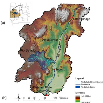
The R´ıo Salado, located in central New Mexico, is part of the Middle R´ıo Grande basin, and extends into Catron, Ci-bola, and Socorro counties (Fig. 1). The basin is selected for this study due to its historical stream gauge located near its confluence with the R´ıo Grande, its semiarid nature and its significant size (3610 km2). The maximum elevation in the R´ıo Salado is 3060 m in the Magdalena Mountains and drops to 1430 m near the outlet to the R´ıo Grande. The stream network consists of a wide, braided channel near the outlet and narrow, incised channels in the headwaters (Nardi et al., 2006). While the R´ıo Salado does not contribute large vol-umes of water to the R´ıo Grande, it does contribute a great deal of sediment (Simcox, 1983) and is similar, in this re-spect, to its neighboring basins (Newman et al., 2006; Vivoni et al., 2006).
The basin extent for the R´ıo Salado was delineated from US Geological Survey (USGS) 30-m elevation data. Fig-ure 1 shows the R´ıo Salado basin and stream network over-laying the Digital Elevation Model (DEM) of the Middle R´ıo Grande. The stream network delineation was achieved
us-Fig. 1. (a)R´ıo Salado basin in New Mexico, along with highlighted counties of Catron, Cibola, and Socorro.(b)30-m digital elevation model (DEM) of the Middle R´ıo Grande basin, with the highlighted R´ıo Salado watershed.
ing the single flow direction algorithm of O’Callaghan and Mark (1984). We found that a stream threshold of 0.5 km2 matched the National Hydrography Dataset (NHD) data well with drainage density of 1.1 (km−1), while minimizing the introduction of first order streams. For visualization purposes in Fig. 1, a threshold of 36 km2 for the stream network is shown.
2.2 Hydrologic response units
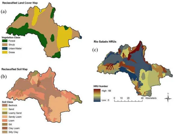
For modeling the R´ıo Salado, the domain defined by the basin boundary was divided into Hydrologic Response Units (HRUs). An HRU is a contiguous unit with a unique combi-nation of soil and vegetation characteristics which are treated as homogeneous (e.g., Kite, 1993; Liang et al., 1994; Arnold et al., 1998). HRUs are often used as a finer discretization of a coarse, grid-based model domain or when computational efficiency is sought. The HRU concept is applied here using the State Soil Geographic (STATSGO) Data Base and the General Vegetation Map of New Mexico. Since each HRU has distinct soil and vegetation characteristics, we assume that landscape properties within each HRU are spatially uni-form. This assumption is motivated by the desire to decrease the computational burden of the model to allow long-term simulations on a personal computer, for the purpose of use in a decision support system (Tidwell et al., 2004).
(a)
(b)
(c)
Fig. 2.Reclassified regional(a)vegetation and(b)soil maps are combined to produce(c)a Hydrologic Response Unit (HRU) distribution for the R´ıo Salado.
Table 1. Percentage of basin area in the R´ıo Salado (total area of 3610 km2) for each coarse soil and vegetation classification.
Soil Class Area (%) Vegetation Area (%) Class
Bedrock 38.43 Forest 23.73 Sand 0.22 Grass 20.83 Loamy sand 3.08 Shrub 55.44 Sandy loam 28.67 Urban/Water <0.01 Loam 27.46
Silt loam 1.01 Clay loam 1.03 Silty clay loam 0.10
the total basin occupied by the soil and vegetation classifica-tions. In general, the basin is dominated by shrublands un-derlain by clay loam soil (19%), and grasslands unun-derlain by sandy loam soil (9.5%). The majority of the HRUs are small in size, each with an area less than 1% of the total R´ıo Sal-ado watershed. However, when the seven largest HRUs are combined,∼10% of the total number of HRUs, these cover ∼65% of the basin area. Field visits were performed for the major units to confirm the accuracy of the HRU delineations used in the model (Arag´on, 2008).
2.3 Rainfall generation
Due to the scarcity of long-term observations, watershed models often use synthetic rainfall as forcing. In this study, a stochastic rainfall model based on Eagleson (1978) was im-plemented to create a time series of rainfall input. The rain-fall model has been widely applied in earlier studies (e.g., Rodr´ıguez-Iturbe and Eagleson, 1987; Tucker and Bras, 2000). The stochastic model samples separate exponential distributions of the storm intensity (I), storm duration (DS)
and inter-storm duration (DI S) as follows:
f (I )= 1 Ie
−I
I
, (1)
f (DS)=
1
DS
e
−DS
DS
, and (2)
f (DI S)=
1
DI S
e
−DI S
DI S
, (3)
whereI,DS, andDI Srepresent mean values for each
param-eter. Deriving these mean values from historical data mimics local conditions using the available observations. Sampling theDS andDI S distributions allows defining a sequence of
the sequence is used in the watershed model as an individual time step to resolve storm and inter-storm hydrologic pro-cesses (e.g., Tucker and Bras, 2000).
Five rain gauges were used to condition the stochastic model: Agustin, Brushy Mountain, Datil, Laguna, and So-corro (Fig. 3). Each gauge provides hourly measurements with record lengths varying from 4 to 30 years (Table 2). The records were used to identify consecutive rainfall periods, es-timate their average intensity over the event duration and de-termine the inter-storm duration between events. Some of the datasets are of limited lengths, may not be completely representative of the historical rainfall at their respective lo-cations or may exhibit problems of precipitation undercatch in unshielded rain gauges, particularly under high wind con-ditions. In addition, the minimum resolution of many of the rain gauges was increased from 0.254 to 2.54 mm during the record period. As a result, higher resolution periods, typi-cally 30 years in length, were used to extract the mean values of each parameter. The assumption of the exponential dis-tributions was verified with the rain gauge data and found to be appropriate for our purposes, though some extreme events are not captured adequately (Arag´on, 2008).
The assignment of each HRU to a particular rain gauge was determined by creating Thiessen polygons around each rain gauge (Fig. 3). Spatial rainfall variability was not al-lowed within each Thiessen polygon. The majority of the basin is located in the boundaries for the Agustin (24.3%), Datil (37.3%), and Socorro (22.2%) sites, with smaller areas for Brushy Mountain (11.0%) and Laguna (5.2%). HRUs overlain by more than one gauge were given parameters of the dominant site. A comparison of the monthly mean pa-rameters for each rain gauge is shown in Fig. 4. Strong seasonality in the parameters is apparent in all five sites. The seasonality is best observed when comparing the win-ter months (December–February) with the summer months (July–September). Comparison among the rain gauges sug-gests that rainfall has more significant seasonal changes as compared to spatial variations among sites. Nevertheless, the rain gauge locations do not entirely capture the precipita-tion variability in the basin, as estimated by the mean annual precipitation in Fig. 3 from the PRISM product (Daly et al., 1994).
2.4 Hydrologic model development
Hydrologic processes in the model are tailored for semiarid basins with diverse soil and vegetation properties. The model commences with the partitioning of rainfall and snow and proceeds to interception by the plant canopy. Water that is able to bypass the canopy and reach the land surface either infiltrates into the soil or becomes runoff that is routed to the basin outlet through the channel network. Two major runoff mechanisms are captured, infiltration- and saturation-excess runoff, derived by tracking the infiltration capacity and sat-urated area fraction of an HRU. Evapotranspiration affects
Fig. 3.Location of the rain gauges near the R´ıo Salado basin along with the associated Thiessen polygon relative to the basin bound-ary. The mean annual precipitation (1971–2000) from PRISM (Precipitation-elevation Regressions on Independent Slopes Model) is shown.
each portion of the hydrologic system, while losses to the regional aquifer are accounted for from the soil column and the channel network. Additional details on the model devel-opment are presented in Arag´on (2008).
In the following, we present a brief description of the model processes. It is important to reiterate that the model is intended to operate at coarse scales to reduce computa-tional burden for long-term and multiple simulations in a de-cision support environment. The spatial scale was coarsened through the HRU discretization, while the temporal scale was aggregated by using storm and inter-storm sequences as time steps. This choice was preferred over a monthly time step to capture the short-term runoff events experienced in semiarid regions (Newman et al., 2006; Vivoni et al., 2006). Never-theless, use of the coarse HRUs and event-based time step imply that the model formulation will have limits in terms of capturing fine-resolution behavior.
2.4.1 Snow accumulation and melt
Snow accumulation is treated as a water balance where the change in snow pack (1SSnow) is the difference between the
volumes of falling snow (VN S) and snowmelt (VM):
1SSnow
1t =
VN S−VM
Table 2.Characteristics of rain gauges near the R´ıo Salado from the National Climatic Data Center (NCDC) and Western Regional Climate Center (WRCC).
Rain gauge Agustin Brushy Datil Laguna Socorro Mountain
Longitude (dd) −107.617 −107.848 −107.766 −107.367 −106.883 Latitude (dd) 34.083 34.719 34.289 35.033 34.083 Elevation (m) 2133.6 2670.7 2316.5 1773.3 1397.5 Record lengths 1948–2007 1992–2007 2003–2007 1946–2006 1948–2006 Resolution (mm) 0.254 0.254 0.254 0.254 0.254 Source NCDC WRCC WRCC NCDC NCDC
Fig. 4.Comparison of the estimated, monthly precipitation param-eters at the rain gauges sites: (a)Storm intensity, I(mm/hr), (b)
Storm duration,Ds (hr) and (c)Inter-storm duration,DI S (day).
Solid lines represent the monthly average values at all rain gauge sites.
To determine the volume of snowfall, a temperature-based allocation method was used to partition a portion of the pre-cipitation as snowfall using a threshold valueTb=−0.5◦C as:
Sf =
Tb−Tmin
Tmax−Tmin, (5)
Sf =1, if Tmax≤Tb, and (6)
Sf =0, if Tmin≥Tb, (7)
whereSf is the fraction falling as snow (Federer et al., 2003),
andTmaxandTminare minimum and maximum air
tempera-tures sampled from an exponential distribution as:
f (T )= 1 Te
−T
T
, (8)
whereT is the mean monthly temperature obtained from his-torical records at each rain gauge. Snowmelt is based on the degree-day method of Martinec et al. (1983) as:
VM =Mf(Ti−Tb), (9)
whereMf=0.011ρs (m3/◦C) is an empirical melt factor,Ti
is the index air temperature (◦C) set to the average ofT
max
andTmin, and ρs is the snow density (assumed constant at
100 kg/m3here).
2.4.2 Canopy interception
Rainfall interception is computed by tracking the change in canopy storage (1SC) as the difference between intercepted
water (VInt), canopy evaporation (VCE) and canopy drainage
(VD):
1SC
1t =
VInt−(VCE+VD)
1t . (10)
The total volume of water intercepted during a storm event (VInt) is computed as:
VInt=IRAvegD, (11)
whereAveg=pvegA,pvegis the vegetated fraction,Ais the total area,D is the duration of the rainfall event, andIR is
the rainfall interception rate by leaves calculated as:
IR=FIntL(LAI)P , (12)
whereFIntLis the fraction of rainfall intercepted by leaves,
assumed to be 0.1pveg,P is the rainfall rate, and LAI is the
leaf area index (Federer et al., 2003). The canopy intercepts water until the maximum canopy storage volume (VCS) is
reached:
VCS=ICLAvegLAI, (13)
where ICL is the leaf interception capacity. Once the
canopy is full, further water input to the canopy is released as drainage (VD). The unintercepted water (VU), which
falls over non-vegetated areas and immediately reaches the ground surface, is calculated as:
whereVP is the rainfall volume. The canopy evaporation
(VE) is computed using the potential evaporation rate as
dis-cussed in the following. 2.4.3 Evapotranspiration
To reduce data requirements, the Hargreaves model was used to estimate the potential evapotranspiration (EH)
(Har-greaves et al., 1985; Har(Har-greaves and Allen, 2003) as:
EH =0.0023 [So(T +17.8)]T
1 2
R, (15)
whereEHis based on the amount of incoming solar radiation
(So, mm/day),T is the mean monthly air temperature (◦C),
andTRis defined as:
TR=Tmax−Tmin. (16)
The amount of incoming solar radiation that reaches the land surface is estimated using the method described by Shuttle-worth (1993):
So=15.392{dr[ωSsin(φ)sin(δ)+cos(φ)cos(δ)sin(ωS)]},(17)
wheredr is the relative distance between the Earth and Sun,
ωSis the sunset hour angle (radians),φis the latitude of the
study area (radians) andδis the solar declination angle (ra-dians). The following equations describe the computation of the solar radiation factors:
dr =1+0.033 cos
2π
365J
, (18)
ωS=arccos(−tan(φ)tan(δ)), and (19)
δ=0.4093 sin
2π
365J−1.405
, (20)
whereJ is the Julian day, set to the 15th day of each month for monthly calculations.
The potential evapotranspiration (EH) is applied to the
canopy (VCE) for the given amount of water available in
canopy storage (Sc) such thatVCE=min(Sc, EH). For high
values ofEH, the canopy storage will quickly be evaporated
during inter-storm periods. Actual evapotranspiration (Ea)
from soil evaporation and plant transpiration is limited by soil water availability and vegetation rooting depth (assumed as 1.5 m). The portion ofEa due to soil evaporation occurs
at a reduced rate for unsaturated soils as:
Ea =EHAsf +EH(A−Asf)
θ
i−θr
θs −θr
, (21)
whereAsf is the saturated area (described below),θi is the
current water content, andθr andθs are the residual and
sat-urated water contents. Following Salvucci (1997), the value of Ea is reduced toER when the inter-storm period (ti) is
greater than two days as:
ER =
1
2(Ea+ET2) , (22)
whereET2is defined as: ET2=0.811Ea
48
ti
. (23)
This reduction is implemented sinceEais controlled by the
rate at which the soil can conduct water to the surface for drying soils. The actual evapotranspiration related to plant transpiration is parameterized in a similar fashion as (Eq. 21) over the soil layers that include plant roots. The plant rooting depth (Zr) is assumed as 1.5 m in this study to include all soil
layers.
2.4.4 Runoff generation and soil moisture redistribution
Water inputs that reach the soil surface are allocated depend-ing on the state of the hydrologic system. The water bal-ance at the land surface is conceptualized after the Three-Layer Variable Infiltration Capacity (VIC-3L) model of Liang et al. (1994, 1996), modified to account for infiltration-excess runoff (RI). If the water input rate is greater than
the saturated hydraulic conductivity of the soil (KS), then
infiltration-excess runoff (RI) will occur as:
RI =w−KS if w > KS, (24)
wherew is the water application rate accounting for unin-tercepted water (VU), canopy drainage (VD) and snowmelt
(VM). The VIC-3L model assumes the degree of saturation
varies spatially and thus saturation-excess runoff (RS) occurs
over the saturated fraction (Asf) as:
RS =wAsf. (25)
The saturated area fraction is obtained as:
Asf =1−
1− ic
im
b
. (26)
where b is the saturation shape parameter (b=1.4 in this study),icis the current infiltration capacity andimis the
max-imum infiltration capacity, determined for the top two layers as:
im=Vm(1+b) , (27)
whereVm=φ−θr is the available volume of the top two soil
layers, calculated as the difference between porosity (φ) and
θr. After some manipulation (Arag´on, 2008),ic can be
ob-tained as:
ic=
( 1−
1−θi−θr φ−θr
1+1b)
, (28)
whereθi is the current water content. As a result,Asf and
iccan be estimated dynamically in the model. The reader is
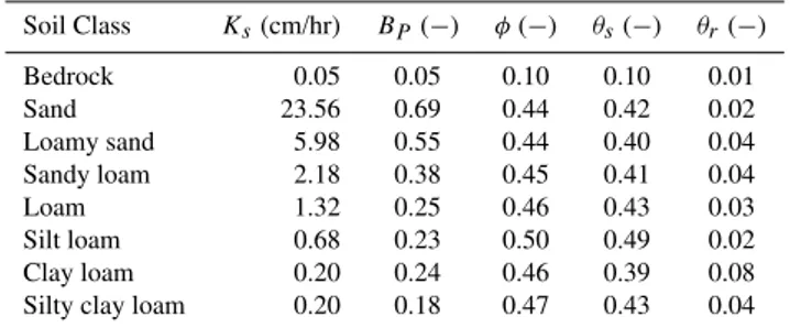
Table 3.Model parameters for the R´ıo Salado soil classes.
Soil Class Ks(cm/hr) BP (−) φ(−) θs(−) θr(−)
Bedrock 0.05 0.05 0.10 0.10 0.01
Sand 23.56 0.69 0.44 0.42 0.02
Loamy sand 5.98 0.55 0.44 0.40 0.04
Sandy loam 2.18 0.38 0.45 0.41 0.04
Loam 1.32 0.25 0.46 0.43 0.03
Silt loam 0.68 0.23 0.50 0.49 0.02
Clay loam 0.20 0.24 0.46 0.39 0.08
Silty clay loam 0.20 0.18 0.47 0.43 0.04
The 1.5 m soil column is divided into three layers with to-tal depths of 10 cm (top), 40 cm (middle) and 100 cm (bot-tom). Direct evaporation from the soil occurs from the top and middle layers, while transpiration is allowed over the plant rooting depth. For each layer, we track the changes in soil moisture storage. For the top layer volume (VTop):
1VTop
1t =
(VInf+VDiM)−(VET+VTT+VDM+VR)
1t , (29)
whereVInfis the infiltration volume related to the water ap-plication rate (w),VDiM andVDM are the volumes that
dif-fuse from and drain to the middle layer, VET andVTT are volumes lost to evaporation and transpiration, andVR is the
total runoff volume (sum ofRSandRI). Similar expressions
are derived for the middle and lower layers. It is important to note that the lower layer has free drainage (D) to the regional aquifer.
Movement of water between the soil layers (Qz) takes into
account the unsaturated hydraulic conductivity (Ku) as:
Qz=AKu=AKs
θ
f −θr
φ−θr
m
, (30)
wherem=3+2/Bp,Bpis the pore size distribution index, and
θf is the adjusted water content at the end of a storm or
inter-storm period defined as:
θf =θr+
(
[θi−θr]1−m−
(
1−m)Ks1t
zi(φ−θr)m
1/(1−m))
,(31) where1tis the length of the period under consideration and
zi is the depth of the soil layer under consideration. The
adjusted water content was computed in order to account for the event-based time step (see Arag´on, 2008 for derivation). 2.4.5 Channel routing
Runoff produced in individual HRUs is routed to the basin outlet along the different flowpaths. To reduce computations, the average flow distance for each HRU to the basin outlet is used to route runoff. The residence time of water in the channel (tc) is defined as:
tc=
LOut
V
, (32)
Table 4.Model parameters for the R´ıo Salado vegetation classes.
Vegetation Class pveg(−) LAI (−) ICL(mm) Zr (m)
Forest 0.60 6 4.5 1.5 Grass 0.75 3 1.9 1.5 Shrub 0.30 3 1.1 1.5 Urban/Water 0 0 0 0
where LOut is the average distance to the outlet for each
HRU, andV is the average flow velocity, set to 0.5 m/s for this study. The channel bed is treated as a soil with variable properties and the volume of water lost in the channel (VLoss)
is calculated as:
VLoss=KStCLOutcW, (33)
wherecW is the average channel width, set to 5 m for this
study. This simple calculation assumes independent flow paths from each HRU to the outlet and may lead to over-estimates of channel losses, but allows channel routing to be handled in a parsimonious fashion.
2.5 Numerical experiments
The semi-distributed watershed model is applied to the R´ıo Salado using either: (1) the historical rain gauge records, (2) the stochastic rainfall model conditioned on historical data, or (3) the long-term scenarios considering changes in precip-itation and temperature. Simulations typically span 40 to 60 years to encompass the historical record or capture long-term climate trends. We conduct simulations on a personal com-puter with an approximate run time of 15-min for a 60-year period. For all simulations, we utilize the HRU spatial dis-cretization depicted in Fig. 2, with an identical set of model parameters (e.g., soil, vegetation and channel properties). Ta-bles 3 and 4 present the assigned model parameters for each soil and vegetation classification in the basin. Our numer-ical experiments do not focus on the potential uncertainties associated with the model parameters. Instead, we minimize model calibration by selecting effective parameters at HRU-scale based on published literature values (e.g., Rawls et al., 1983; Bras, 1990; Dingman, 2002; Federer et al., 2003; Cay-lor et al., 2005; Guti´errez-Jurado et al., 2006).
(e.g., Small and Kurc, 2003). At the HRU-scale, compar-isons between a forested, sandy HRU and a grassy, clay HRU in the R´ıo Salado allowed inspection of the hydrologic dy-namics during a wet and a dry year (not shown). A full suite of model outputs for each HRU, including interception, soil moisture, evapotranspiration and runoff dynamics, exhibited physically reasonable differences that were directly related to the model parameterizations in Tables 3 and 4. The lack of hydrologic data in the R´ıo Salado prevents a more detailed model comparison.
For the long-term simulations, we initialize the watershed model with residual soil moisture (θr) in each HRU to
de-pict the dry state in the semiarid region. For each simu-lation, we conduct a 10-year model spin-up, with precipi-tation and temperature forcing, to allow the basin to reach quasi-equilibrium conditions in terms of the root zone soil moisture. To account for the stochastic nature of the climate forcing, we also carry out twenty-five realizations (ensem-ble members) for each scenario. This allows quantifying the ensemble mean behavior as well as the uncertainty (ensem-ble standard deviation) associated with the hydrologic model response. While the ensemble size is small, the long simu-lation duration (60-year) and the storm and interstorm event time step ensure a large sample size of wet and dry periods in each ensemble member. We separately assess the impact of changes in precipitation (storm intensity and inter-storm duration) along with temperature changes in the R´ıo Salado basin, as detailed in Sect. 3.
We focus primarily on the sensitivity of the hydrologic re-sponse to the climate scenarios at the catchment outlet due to: (1) the need for streamflow predictions in ungauged trib-utaries of the R´ıo Grande, (2) the linkage of the watershed model with the decision-support tool of Tidwell et al. (2004) through tributary inflows, and (3) the restricted resolution of the semi-distributed, event-based model (see Arag´on et al., 2006 for an illustration of the spatial runoff production). While detailed spatial analyses of the hydrologic response are limited, the model resolution does allow for an improved representation of semiarid processes, as compared to lumped, monthly models. This is primarily due to the improved abil-ity of semi-distributed models to capture the response to summer storms in the region, as discussed in Michaud and Sorooshian (1994).
3 Results and discussion
3.1 Comparisons to historical streamflow observations
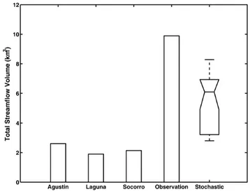
A streamflow gauge, operational at the R´ıo Salado near San Acacia, NM (34◦17′50′′N, 106◦53′59′′W, USGS 08354000) during the period 1947–1984, allows comparison with the model simulations applied at the basin-scale. The availabil-ity of the historical rainfall data at three rain gauges (Socorro, Laguna, Agustin) limits the simulation period to 1949–1978
Fig. 5. Total streamflow volumes (km3) for the R´ıo Salado basin from deterministic model simulations with uniform forcing at the Agustin, Laguna and Socorro rain gauges; historical observations at the streamflow gauge; and the ensemble model simulations us-ing the stochastic rainfall model (twenty-five realizations) over the 30-year period (1949–1978). Note that the stochastic model results are shown as a box-and-whisker plot, with the median of the dis-tribution (horizontal line), the lower and upper quartiles (box) and the maximum and minimum values (vertical bars). The notch rep-resents a robust estimate of the uncertainty around the median.
(i.e., due to the reduction in rainfall precision). Note that this period coincides with a single phase of the Pacific Decadal Oscillation (PDO) and a range of different ENSO conditions, which have been shown to influence precipitation in the re-gion (Guan et al., 2005). No other rainfall observations are available for this historical period, limiting our ability to pro-vide distributed forcing to the model. The rainfall amounts at these sites should underestimate the total rainfall in the basin, as these are located in the lower elevations of the region. For example, Fig. 4 indicates that while the mean rainfall inten-sities for the Brushy Mountain and Datil rain gauges, located at higher elevations, are similar to the other gauges, the inter-storm periods are significantly shorter.
Figure 5 compares the observed streamflow volume (km3) over the 30-year period with model simulations assuming spatially-uniform rainfall forcing from each rain gauge in-dividually (i.e., without the Thiessen polygons shown in Fig. 3). Thus, for example, the label “Agustin” implies that uniform forcing from the Agustin rain gauge was used to force the model in a spatially uniform fashion. Historical records at each rain gauge site were classified into storm and inter-storm periods, characterized by DS, DI S and I,
1
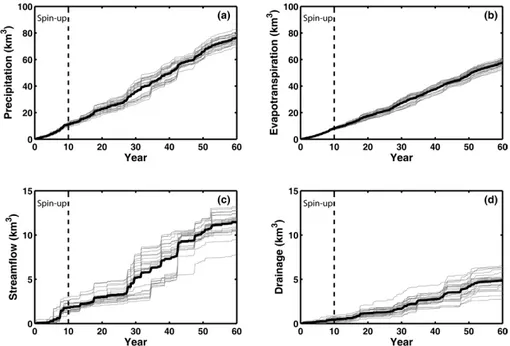
Fig. 6. Basin-scale water balance components in the R´ıo Salado based on twenty-five ensemble runs shown as cumulative volumes over the 60-year simulation, with a 10-year model spin-up:(a)Precipitation (km3),(b)Evapotranspiration (km3),(c)Streamflow (km3), and(d)
Drainage (km3). The thick lines in each denote the cumulative ensemble means.
captured in the stochastic rainfall model (i.e., due to the as-sumption of the exponential distribution of the model param-eters, see Arag´on, 2008), do not bias the comparison between the observations and model simulations. The streamflow from only one year (1972) exceeded this criterion (3.07 km3 which is seven times the long-term mean or +5 standard de-viations from the mean) and was excluded from the observa-tions in Fig. 5. Clearly, the use of an extreme value distribu-tion for the stochastic rainfall model (e.g., the Gumbel dis-tribution, see Bras, 1990) could help capture this rare flood event.
Comparison of the model simulations obtained from the spatially-uniform forcing and the historical observations in-dicate a significant underestimation of the total streamflow volume in the R´ıo Salado. The model simulations from the uniform forcing at the three low elevation gauges arithmeti-cally average 2.22 km3, while the historical observations in-dicate 9.89 km3. This is primarily due to rainfall underesti-mation in the higher elevations of the basin, where precipi-tation data is unavailable. For example, Fig. 3 indicates that the mountainous basin regions receive∼400 to 460 mm/year, while the Laguna, Socorro and Agustin sites only have ∼240 to 330 mm/year. Clearly, the use of low-elevation rain gauge forcing does not lead to simulated streamflow volumes that are comparable to historical data. To achieve the ob-served volumes, while maintaining an annual runoff ratio of 15% (a reasonable approximation), a precipitation volume of 65.93 km3is required. This suggests that the lower elevation rain gauges only account for∼32% of the precipitation in the R´ıo Salado basin for the assumed runoff ratio.
3.2 Analysis of long-term ensemble simulations
The long-term ensemble simulations aid to quantify how pre-cipitation seasonality and interannual variations influence the basin hydrologic response in the R´ıo Salado. Recall the stochastic simulations are conditioned on the spatiotemporal variations in precipitation intensity, duration and frequency, as well as the temperature seasonality, from the five rain gauges. The twenty-five realizations are generated by sam-pling the exponential distributions describing the precipita-tion (Eqs. 1–3) and temperature (Eq. 8) forcing with a dif-ferent random seed for each ensemble member. Thus, the forcing for the long-term simulations represents climate un-certainty through the sampling of the underlying statistical distributions. Figure 6 presents the cumulative volumes of precipitation (P), evapotranspiration (ET), streamflow (Q) and drainage (D) over the 60-year simulations. Note that the cumulative precipitation, streamflow and drainage series exhibit both seasonal and interannual variations, as shown by the variable stair-step behavior. Inspection of the final ensemble mean cumulative volumes indicates that the evap-otranspiration ratio (ET/P) of 75.3% and runoff ratio (Q/P) of 14.9% are consistent with the semiarid nature of the R´ıo Salado. The remaining amount is partitioned to regional drainage (D/P=6.4%) and small increases in soil moisture storage. These results are comparable to Li et al. (2007) who foundET/P=82.3% over a 5-year period in the R´ıo Grande, using a high-resolution model.
Cumulative water balance components reveal the punc-tuated, but frequent, streamflow events in the R´ıo Salado (Fig. 6c), while drainage occurs infrequently (Fig. 6d) when saturation allows transport beyond the root zone. Clearly, streamflow and drainage are of lower magnitude and fre-quency as compared to the consistent losses toET (Fig. 6b). This is supported by studies indicating highET and lower streamflow and drainage pulses in the R´ıo Salado (e.g., New-man et al., 2006; Sandvig and Phillips, 2006). Neverthe-less, the ensemble mean Q/Pand D/Pfrom the watershed model exceed previous estimates, for example by Grimm et al. (1997) (Q/P=<5%), Gochis et al. (2003) (Q/P=<2%, D/P=<2%) and Li et al. (2007) (Q/P=<2%). These low es-timates are inconsistent with the long-term streamflow data (0.43 km3/year) and the basin-averaged annual precipitation from PRISM (342 mm or 1.23 km3 over the basin, Fig. 3), which yield Q/P=34.8%. As a result, the model estimate (Q/P=14.9%) is closer to the long-term runoff ratio, while preserving the highET/P, as compared to previous studies in the region.
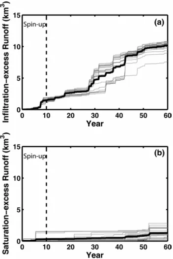
Figure 7 compares the cumulative volumes of the infiltration-excess (RI) and saturation-excess (RS) runoff
mechanisms over the 60-year ensemble simulations. This comparison is a useful diagnostic tool to assess how the pre-cipitation forcing is converted into streamflow. The final en-semble mean cumulative volume forRI(10.19 km3) exceeds
RS (1.31 km3) by nearly an order of magnitude. This
indi-Fig. 7. Same as Fig. 6 but for(a)Infiltration-excess runoff (km3) and(b)Saturation-excess runoff (km3).
cates that infiltration-excess is the dominant mechanism in the watershed model (88.5% of total streamflow), consistent with the conceptualization of runoff in semiarid basins (e.g., Beven, 2002; Newman et al., 2006; Vivoni et al., 2006). This implies that precipitation intensities, primarily during the North American monsoon (Fig. 4), exceed the soil in-filtration capacity (Table 3) and are responsible for the ma-jor flood pulses. Saturation-excess runoff is less common due to the infrequent occurrence of saturated soil conditions. Furthermore, the variation among the ensemble members ap-pears to be greater forRS as compared to RI, suggesting
that fully-saturated soil conditions can occur in particular in-stances in the simulations.
To further quantify the variations among the ensemble members, Table 5 presents ensemble statistics for the water balance components (P,ET,QandD) and runoff mecha-nisms (RI andRS): ensemble mean (µE), standard
devia-tion (σE), and the coefficient of variation (CV=σE/µE) at the
end of the simulation period. The ensembleσE andCV are
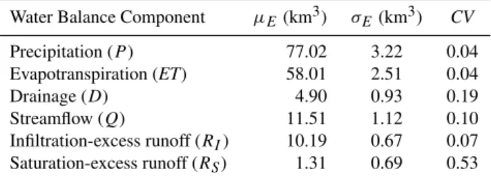
Table 5.Ensemble mean (µE), standard deviation (σE) and
coeffi-cient of variation (CV) of water balance component volumes (km3) at the end of the 60-year simulations.
Water Balance Component µE(km3) σE(km3) CV
Precipitation (P) 77.02 3.22 0.04 Evapotranspiration (ET) 58.01 2.51 0.04 Drainage (D) 4.90 0.93 0.19 Streamflow (Q) 11.51 1.12 0.10 Infiltration-excess runoff (RI) 10.19 0.67 0.07
Saturation-excess runoff (RS) 1.31 0.69 0.53
respect to precipitation (CV=0.04), indicates the hydrologic variable has greater relative variations in the ensemble. Thus, the uncertainty in the precipitation forcing is amplified in the hydrologic response. For example, streamflow (CV=0.10) and drainage (CV=0.19) are more variable as compared to precipitation, whileET (CV=0.04) has similar relative vari-ability. Clearly, evapotranspiration is primarily subject to un-certainty in precipitation.
A close comparison of the relative variability of the infiltration- and saturation-excess runoff in Table 5 further highlights the propagation of precipitation uncertainty in the hydrologic model. WhileRI has a larger ensemble mean,
it exhibits significantly lowerCV as compared toRS. This
suggests that threshold runoff processes that are dependent on both precipitation and the degree of soil saturation have greater variability in a semiarid region where the soils are usually dry. Note that the variability in RS is responsible
for a large proportion of the streamflowCV, in particular for the early period of the simulation (Fig. 6). Similarly, the drainage process exhibits a large ensemble variation since it depends on having saturated conditions in the soil profile. This analysis indicates the model can amplify the precipita-tion uncertainty in the hydrologic response due to the nonlin-ear and threshold nature of the underlying processes. 3.3 Analysis of precipitation and temperature change
scenarios
Considerable debate still exists with respect to the anticipated climate changes for the Southwest US. For example, Serrat-Capdevila et al. (2007) found a wide variation in rainfall pro-jections (from∼100 to 510 mm/year by the year 2100) in the San Pedro basin (AZ) from 17 simulations. Given this range of climate change projections, we identified two observed precipitation trends that could be imposed to the watershed model as the basis for constructing climate scenarios: (1) a decrease in the winter inter-storm duration,DI S(Moln´ar and
Ram´ırez, 2001; Hamlet and Lettenmaier, 2007), and (2) an increase in the summer storm intensity, I (Diffenbaugh et al., 2005; Peterson et al., 2008). We selected the months of December to February (DJF) and July to September (JAS)
to represent the two seasons. The months of JAS are an ap-propriate selection for the summer period in the region as it coincides with the extent and duration of the North Amer-ican monsoon (Douglas et al., 1993). Percentage changes (%) in the mean monthlyDI S andI were applied at all rain
gauge sites during the long-term simulations. These percent-age changes were selected in order to: (1) span a range of impacts on the total precipitation, up to a doubling ofP; (2) test the variation ofDI S andI in the direction of the
an-ticipated change and beyond the observed values in Fig. 4, and (3) retain the spatial variability in the rainfall parameters. We refer to percentage decreases inDI S as “winter
scenar-ios” and increases inI as “summer scenarios” in the follow-ing discussion. Clearly, both hypothesized scenarios lead to increases in the total precipitation volume in the basin, but vary with respect to the seasonal distribution and precipita-tion characteristic (intensity, duraprecipita-tion and frequency). While shorter inter-storm durations or higher intensities are possi-ble, the winter and summer scenarios should capture trends due to higher precipitation that reveal anticipated catchment behavior.
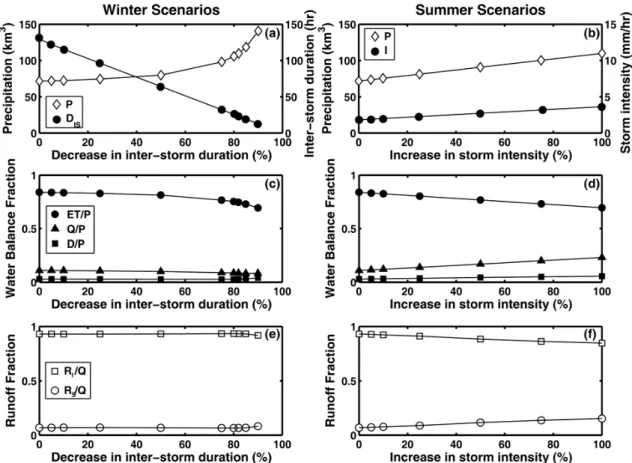
Figure 8 presents the variation in the precipitation forc-ing for the winter and summer scenarios derived from a se-quence of long-term (60-year) simulation. For the winter scenarios, the station-averaged inter-storm duration is de-creased from the nominal value (DI S=129.7 hr) to a
mini-mum value (DI S=12.8 hr, 90% decrease). This decrease in
DI Sresults in a nonlinear increase in precipitation from 71.6
to 140.6 km3(Fig. 8a). For the summer scenarios, the station-averaged storm intensity is increased from the nominal case (I=1.8 mm/hr) to a maximum value (I=3.6 mm/hr, 100% in-crease). Increasing storm intensity results in a linear precip-itation increase from 71.6 to 109.8 km3(Fig. 8b). The sce-narios indicate that precipitation sensitivity varies as a func-tion of the parameter changes. To reach a common basis for comparison, we selected cases with matching total precipi-tation volume (P=109.7 km3): (1) a 82% decrease in winter inter-storm duration (DI S=23.1 hr), and (2) a 100% increase
in summer intensity (I=3.6 mm/hr). The matching cases are used to carry out ensemble simulations that compare the ef-fects of seasonal precipitation variations.
The impacts of precipitation changes on the water balance fractions (ET/P,Q/PandD/P) and the runoff fractions (RI/Q
andRS/Q)are shown in Fig. 8. Increases in winter
precip-itation induced by lowerDI S yield reductions inET/Pand
1
2
Fig. 8.Winter and summer precipitation change scenarios.(a)Precipitation volume (P, km3) and inter-storm duration (DI S, hr) as function
of the decrease inDI S (%) for winter scenarios. (b) Precipitation volume (P, km3) and storm intensity (I, mm/hr) as function of the
increase inI(%) for summer scenarios.(c, d)Water balance fractions (ET/P,Q/P,D/P )for the winter and summer scenarios, whereETis evapotranspiration,Qis streamflow andDis drainage volumes.(e, f)Runoff fractions (RI/Q,RS/Q) for the winter and summer scenarios,
whereRI,RSandQare infiltration-excess, saturation-excess and total runoff.
increase in soil moisture that promotes higher streamflow and drainage. Interestingly, the increase inQwith more intense storms also leads to an increase inRS/Q, due to the presence
of higher levels of soil saturation, thoughRI/Qis still the
dominant mechanism (Fig. 8f). Note that the two matching cases (i.e., winterDI S decrease of 82% and summerI
in-crease of 100%) should have comparableET/P, but differing amounts ofD/P,Q/Pand its partitioning (RI/QandRS/Q),
as explored next.
Figure 9 shows the cumulative water balance volumes ob-tained from twenty-five, long-term simulations performed for the matching winter and summer scenarios. The ensem-ble mean P, ET, Qand D are shown as thick solid lines in Fig. 9. By design, the cumulative precipitation volumes are similar, leading to overlapping envelops (Fig. 9a), though the methods used to achieve this are different. As a result, there are only small variations in the cumulativeET(Fig. 9b) in the scenarios, with the summer (ET/P=63.9%) experienc-ing lowerET as compared to the winter (ET/P=71.5%). The variations in precipitation characteristics, however, lead to significant differences in the streamflow and drainage. Note
that the summer ensemble mean has nearly 2.5 times more
Q(Fig. 9c) and 1.6 times higherD (Fig. 9d) as compared to the winter. In addition, the ensemble streamflow en-velops become distinct and non-overlapping for the summer (Q/P=27.4%) and winter (Q/P=11.1%) scenarios, suggest-ing a fundamental change in runoff production among the scenarios. Drainage differences, on the other hand, are less pronounced as indicated by the slightly overlapping ensem-ble envelopes.
To diagnose the underlying causes for the streamflow dif-ferences, Fig. 10 presents the cumulative volumes of the infiltration- and saturation-excess runoff for the matching cases. Though both ensembles lead to increases inRI and
RSrelative to Fig. 7 (i.e., long-term simulations under
1
Fig. 9.Basin-scale water balance components in the R´ıo Salado for a decrease in winter (DJF) inter-storm duration (blue lines, 82% decrease inDI S) and an increase in summer (JAS) storm intensity (red lines, 100% increase inI). Results are shown as cumulative volumes over the
60-year simulations:(a)Precipitation (km3),(b)Evapotranspiration (km3),(c)Streamflow (km3), and(d)Drainage (km3).
greaterRS, an indication that higher soil moisture occurs in
response to the summer storms, consistent with the higher drainage. The ensemble variations in RI and RS also
dif-fer among the two scenarios, with higher relative variability inRS for the winter and inRI for the summer. This
indi-cates that changes in seasonal precipitation (i.e., more fre-quent winter storms or more intense summer storms) have different consequences on the runoff partitioning in the R´ıo Salado.
The hydrologic effects of the winter and summer scenarios for the matching precipitation volume is further quantified in Table 6. Here, the ensemble mean (µE), standard deviation
(σE), and the coefficient of variation (CV) are presented for
each scenario. An amplification of precipitation uncertainty (CV=0.04 in winter and 0.05 in summer ensembles) is ob-served in the hydrologic response, in particular for drainage, streamflow and the runoff mechanisms. Both scenarios ex-hibit comparable relative streamflow variability (CV=0.09). Nevertheless, changes in winter precipitation lead to greater CVfor hydrologic processes related to thresholds in soil sat-uration (e.g., satsat-uration-excess runoff and drainage). While this is important, it is tempered by the fact that the summer scenarios yield significantly larger µE for streamflow and
drainage, thus having a greater impact on the overall water balance in the R´ıo Salado. Clearly, this comparison indicates that seasonal precipitation trends result in varying hydrologic effects, which argues for a seasonal focus in climate change studies in the region (e.g., Serrat-Capdevila et al., 2007).
The previous analysis has focused exclusively on precip-itation trends for winter and summer periods. An important consideration is the impact of elevated air temperature
result-ing from climate change (e.g., Alexander et al., 2006; Diffen-baugh et al., 2008). In this study, we imposed air temperature increases from 0 to 4◦C by modifying the stochastic temper-ature model for single, long-term realizations of the winter and summer scenarios. Note that these simulations combine the seasonal precipitation trend previously explored with the air temperature increase. Figure 11 presents the limited sen-sitivity of the water balance fractions (ET/P,Q/PandD/P) to the temperature increases in the R´ıo Salado. Slight in-creases inET/P(from 74.6% to 80.0%),Q/P(from 8.5% to 9.5%) andD/P(from 2.9% to 3.4%) are observed for the win-ter scenario, while the summer scenario remains unchanged. The higher winter sensitivity is consistent with the tempera-ture effect on snow accumulation and melt as well as on the relatively higher impact on potentialET. As noted by Serrat-Capdevila et al. (2007), however, a slight increase in temper-ature in semiarid regions may have limited effects onET as the actual rates are limited by soil moisture amounts. As a result, it is clear that the hydrologic model application in the R´ıo Salado is more sensitive to seasonal precipitation trends than to temperature changes.
Table 6.Same as Table 5, but for winter and summer precipitation scenarios.
Water Balance Component Winter Scenarios Summer Scenarios
µE(km3) σE(km3) CV µE(km3) σE(km3) CV
Precipitation (P) 112.99 4.09 0.04 117.51 5.90 0.05 Evapotranspiration (ET) 80.78 3.31 0.04 75.05 3.42 0.05 Drainage (D) 5.21 1.07 0.21 8.27 1.08 0.13 Streamflow (Q) 12.54 1.11 0.09 32.19 3.00 0.09 Infiltration-excess runoff (RI) 11.11 0.67 0.06 27.30 1.88 0.07
Saturation-excess runoff (RS) 1.43 0.68 0.48 4.89 1.61 0.33
sensitivities that begin to mimic the summer scenarios (i.e, lowerET/Pand higherQ/PandD/P). In other words, impos-ing a realistic temperature trend in the R´ıo Salado leads to a more sensitive basin response throughout the year (win-ter and summer), as compared to having no temperature trend. Clearly, the precipitation scenarios tested here are not necessarily mutually exclusive, though we have tested them separately. If more frequent winter storms, more in-tense summer storms and higher temperatures occur simulta-neously, the hydrologic consequences would be compounded as these effects operate in the same direction.
4 Summary and conclusions
Understanding the hydrologic effects of potential climate changes in the Southwest US is challenging due to several factors, including, but not limited to: (1) the complex na-ture of the hydrologic processes in semiarid basins, (2) the inherent climate variability that characterizes the region, (3) the sparse distribution of hydrologic observations, and (4) the uncertainty in climate projections during the two major pre-cipitation seasons. In this study, we developed a watershed modeling tool tailored to the semiarid basins in the South-west US that attempts to capture the various forms of pre-cipitation variability and the dominant hydrologic processes in a simplified and parsimonious fashion. While more com-plex numerical models (e.g., Vivoni et al., 2007; Liuzzo et al., 2009) could represent the climatic forcing and watershed characteristics in greater detail, the computational demands would not facilitate long-term, ensemble simulations of cli-mate change scenarios in a decision support environment (Tidwell et al., 2004). In this respect, the semi-distributed watershed model can ultimately provide predictions that aid in water management and decision making in regions where water is a limited resource.
While there are many applications of the semi-distributed model, this study focuses on evaluating the model sensitiv-ity to imposed precipitation and temperature scenarios in the R´ıo Salado of central New Mexico. The scenarios capture recent evidence for the variation in seasonal precipitation in the Southwest US (e.g., Alexander et al., 2006; Peterson et
Fig. 10. Same as Fig. 9 but for(a)Infiltration-excess runoff (km3) and(b)Saturation-excess runoff (km3).
1 2
Fig. 11. Water balance fractions (ET/P,Q/P, D/P) as a function of an air temperature increase (◦C) for the winter (82% decrease in inter-storm duration) and summer (100% increase in storm intensity) scenarios.
results to similar basins in the region. Results from this study indicate the following:
1. The continuous, semi-distributed watershed model de-veloped for applications in large, semiarid basins in the Southwest US is able to capture the spatial and tempo-ral variations in climate forcing and watershed charac-teristics in a coarse, but parsimonious, fashion. By us-ing Hydrologic Response Units (HRUs) and a storm and inter-storm time step, the model is able to capture brief and intense hydrologic responses to winter and summer precipitation regimes. As a result of the model compu-tational feasibility, long-term ensemble simulations of climate change scenarios are feasible at the basin-scale for use within a decision support environment.
2. Comparisons of the simulated streamflow to the histori-cal gauge record in the R´ıo Salado reveal the difficulties in applying the model with uniform forcing from low-elevation rain gauge sites. Conditioning the stochastic rainfall model with all available rain gauge data leads to measurable improvements in the simulated stream-flow. Long-term ensemble simulations of the historical period also lead to evapotranspiration and runoff ratios that improve previous estimates in the semiarid region. Given the scarcity of accurate precipitation data in the Southwest US, an ensemble-based approach is a useful means for hydrologic assessments in ungauged basins. 3. A hydrologic amplification of the precipitation forcing
uncertainty is observed for historical periods and cli-mate change scenarios. Ensemble statistics reveal this amplification is highest for hydrologic processes depen-dent on a soil saturation threshold, in particular drainage and saturation-excess runoff. Negligible amplification is observed for evapotranspiration due to the low actual rates as compared to the potential values. Precipitation uncertainty propagation also varies among the winter and summer scenarios, indicating that a seasonal focus in climate changes studies is warranted in the region due to the dual nature of the precipitation regime.
4. Precipitation scenarios constructed for the winter and summer capture observed and anticipated trends of more frequent winter storms and more intense summer events in the Southwest US. The hydrologic responses vary for each scenario, with a greater sensitivity of the water balance and runoff partitioning to the sum-mer cases. Ensemble simulations with matching pre-cipitation volumes lead to distinct and non-overlapping streamflow responses in the winter and summer that in-dicate a fundamental change in runoff generation. This is diagnosed as the result of the impact of intense sum-mer storms on infiltration-excess runoff.
5. Combining the precipitation scenarios with increases in air temperature yields small, but measurable effects on the winter hydrologic response, and a minimal impact in the summer. Overall, the hydrologic model applica-tion in the rainfall-dominated R´ıo Salado is more sensi-tive to seasonal precipitation changes than to rising tem-peratures. Imposing a realistic temperature trend, how-ever, leads to a more sensitive basin response through-out the year, as compared to no temperature trend. As a result, the combined precipitation and temperature changes lead to a winter hydrologic response that starts to mimic the summer period.
sparse precipitation network in the region was found to af-fect the model testing against the historical streamflow ob-servations. This data limitation could be remedied by us-ing Next Generation Weather Radar (NEXRAD), develop-ing a temporally-disaggregated PRISM product (G. Klise, personal communication, 2007) or applying a space-time stochastic model (e.g., Mascaro et al., 2008), though the un-derlying lack of rain gauge data and the streamflow period will still impact each approach. Despite these assumptions, the results of this study are useful for understanding the hy-drologic sensitivities to climate change in semiarid basins of the Southwest US where relatively few studies have been conducted (e.g., Christensen et al., 2004; Kim, 2005; Serrat-Capdevila et al., 2007), typically with models having compa-rable sophistication as the approach presented here.
The level of sophistication in hydrologic assessments of climate change impacts could be significantly improved through two avenues: (1) improvements in the computational feasibility of distributed hydrologic models that more faith-fully represent basin properties, meteorological forcing and the underlying processes, for example, Abbott et al. (1986), Wigmosta et al. (1994), and Vivoni et al. (2007), and (2) improvements in regional climate change predictions at the high spatial and temporal resolutions needed to drive basin-scale hydrologic models with their required forcing variables (e.g., Diffenbaugh et al., 2005, 2008). Distributed models, in particular, would provide an opportunity to track the propa-gation of climate scenarios to the hydrologic patterns in the basin, such as soil moisture, runoff production, evapotran-spiration, and channel discharge at internal locations, among others. For example, Vivoni et al. (2009) recently evalu-ated the impact of high-resolution, regional weather forecasts on the spatially-distributed basin response in the R´ıo Puerco basin of north-central New Mexico. In anticipation of these advances, the proposed approach in this study allows inves-tigation of the basin hydrologic response and its sensitivity under seasonal climate scenarios that capture forcing uncer-tainty. In this respect, the major contribution of this study is to identify how observed climate trends in the winter and summer affect the regional water supply. The challenges for water resources management in the face of these hydrologic changes are formidable.
Acknowledgements. We acknowledge funding from the Sandia
Laboratory Directed Research and Development (LDRD), San-dia University Research Program (SURP), New Mexico Water Resources Research Institute, and the Alliance for Graduate Education and the Professoriate which sponsored the M.S. thesis in Hydrology of C. A. Arag´on at New Mexico Tech. We thank G. Klise, R. Mantilla and G. Mascaro for discussions related to the model development efforts in this work. We also thank three anonymous reviewers, G. Mascaro and M. Sivapalan for insightful comments that helped improve the manuscript.
Edited by: M. Sivapalan
References
Abbott, M. B., Bathurst, J. C., Cunge, J. A., O’Connell, P. E., and Rasmussen, J.: An introduction to the European Hydrological System “SHE” 2: Structure of a physically based, distributed modelling system, J. Hydrol., 87, 61–77, 1986.
Ahmad, S. and Simonovic, S. P.: Spatial system dynamics: New ap-proaches for simulation of water resources systems, J. Comput. Civil Eng., 18(4), 331–340, 2004.
Alexander, L. V., Zhang, X., Peterson, T. C., et al.: Global observed changes in daily extremes of temperature and precipitation, J. Geophys. Res., 111, D05109, doi:10.1029/2005JD006290, 2006. Arag´on, C. A., Malczynski, L., Vivoni, E. R., Tidwell, V. C., and Gonzales, S.: Modeling ungauged tributaries using Ge-ographical Information Systems (GIS) and System Dynamics, ESRI International User Conference Proceedings, San Diego, CA, available at: http://proceedings.esri.com/library/userconf/ proc06/papers/papers/pap 1163.pdf, 2006.
Arag´on, C. A.: Development and testing of a semi-distributed wa-tershed model: Case studies exploring the impact of climate vari-ability and change in the R´ıo Salado, M.S. thesis, New Mexico Institute of Mining and Technology, Socorro, NM, USA, 158 pp., 2008.
Arnold J. G., Srinivasan, R., Muttiah, R. S., and Williams, J. R.: Large area hydrologic modeling and assessment Part I: model development, J. Am. Water Resour. As., 34(1), 73–89, 1998. Beven, K. J.: Runoff generation in semi-arid areas, in: Dryland
Rivers, edited by: Bull, L. J. and Kirkby, M. J., John Wiley, Chichester, 57–105, 2002.
Bras, R. L.: Hydrology: An introduction to hydrologic science, Addison-Wesley-Longman, Redding, MA, 1990.
Caylor, K. K., Manfreda, S., and Rodriguez-Iturbe, I.: On the cou-pled geomorphological and ecohydrological organization of river basins, Adv. Water Resour., 28, 69–86, 2005.
Christensen, N. S., Wood, A. W., Voisin, N., Lettenmaier, D. P., and Palmer, R. N.: The effects of climate change on the hydrol-ogy and water resources of the Colorado River basin, Climatic Change, 62, 337–363, 2004.
Daly, C., Neilson, R. P., and Phillips, D. L.: A statistical to-pographic model for mapping climatological precipitation over mountainous terrain, J. Appl. Meteorol., 33(2), 140–158, 1994. Diffenbaugh, N. S., Pal, J. S., Trapp, R. J., and Giorgi, F.:
Fine-scale processes regulate the response of extreme events to global climate change, P. Natl. Acad. Sci. USA, 102(44), 15774–15778, 2005.
Diffenbaugh, N. S., Giorgi, F., and Pal, J. S.: Climate change hotspots in the Unites States, Geophys. Res. Lett., 35, L16709, doi:10.1029/2008GL035075, 2008.
Dingman, S. L.: Physical Hydrology, 2nd edn., Prentice Hall, Upper Saddle River, NJ, 2002.
Douglas, M. W., Maddox, R. A., Howard, K., and Reyes, S.: The Mexican monsoon, J. Climate, 6, 1665–1677, 1993.
Eagleson, P. S.: Climate, soil, and vegetation, 2. The distribution of annual precipitation derived from observed storm sequences, Water Resour. Res., 14, 713–721, 1978.
Ellis, S. R., Levings, G. W., Carter, L. F., Richey, S. F., and Radell, M. J.: Rio Grande valley, Colorado, New Mexico and Texas, Water Resour. Bull., 29(4), 617–646, 1993.
1449–1467, 1994.
Federer, C. A., V¨or¨osmarty, C., and Fekete, B.: Sensitivity of an-nual evaporation to soil and root properties in two models of con-trasting complexity, J. Hydrometeorol., 4, 1276–1290, 2003. Grimm, N. B., Chacon, A., Dahm, C. N., Hostetler, S. W., Lind,
O. T., Starkweahter, P. L., and Wurtsbaugh, W. W.: Sensitiv-ity of aquatic ecosystems to climatic and anthropogenic changes: The Basin and Range, American Southwest and Mexico, Hydrol. Process., 11, 1023–1041, 1997.
Gochis, D. J., Shuttleworth, W. J., and Yang, Z. L.: Hydrometeo-rological response of the modeled North American monsoon to convective parameterization, J. Hydrometeorol., 4(2), 235–250, 2003.
Goodrich, D. C., Unkrich, C. L., Keefer, T. O., Nichols, M. H., Stone, J. J., Levick, L. R., and Scott, R. L.: Event to multi-decadal persistence in rainfall and runoff in southeast Arizona, Water Resour. Res., 44, W05S14, doi:10.1029/2007WR006222, 2008.
Guan, H., Vivoni, E. R., and Wilson, J. L.: Effects of at-mospheric teleconnections on seasonal precipitation in moun-tainous regions of the southwestern U.S.: A case study in northern New Mexico, Geophys. Res. Lett., 32(23), L23701, doi:10.1029/2005GL023759, 2005.
Guti´errez-Jurado, H. A., Vivoni, E. R., Harrison, J. B. J., and Guan, H.: Ecohydrology of root zone water fluxes and soil development in complex semiarid rangelands, Hydrol. Process., 20(15), 3289– 3316, 2006.
Gutzler, D. S.: Covariability of spring snowpack and summer rain-fall across the southwestern United States, J. Climate, 13(22), 4018–4027, 2000.
Hall, A. W., Whitfield, P. H., and Cannon, A. J.: Recent variations in temperature, precipitation and streamflow in the Rio Grande and Pecos River basins of New Mexico and Colorado, Rev. Fish. Sci., 14, 51–78, 2006.
Hamlet, A. F. and Lettenmaier, D. P.: Effects of 20th century warm-ing and climate variability on flood risk in the western U.S., Water Resour. Res., 43, W06427, doi:10.1029/2006WR005099, 2007.
Hargreaves, G. L., Hargreaves, G. H., and Riley, J. P.: Irrigation water requirements for Senegal River basin, J. Irrig. Drain. E.-ASCE, 111(3), 265–275, 1985.
Hargreaves, G. H. and Allen, R. G.: History and evaluation of Har-greaves evapotranspiration equation, J. Irrig. Drain. E.-ASCE, 129(1), 53–63, 2003.
Lettenmaier, D. P., Wood, A. W., Palmer, R. N., Wood, E. F., and Stakhiv, E. Z.: Water resources implications of global warm-ing: A U.S. regional perspective, Climatic Change, 43, 537–579, 1999.
Li, J., Gao, X., and Sorooshian, S.: Modeling and analysis of the variability of the water cycle in the Upper Rio Grande basin at high resolution, J. Hydrometeorol., 8, 805–824, 2007.
Liang, X., Lettenmaier, D. P., Wood, E. F., and Burges, S. J.: A sim-ple hydrologically based model of land surface water and energy fluxes for general circulation models, J. Geophys. Res., 99(D7), 14415–14428, 1994.
Liang, X., Wood, E. F., and Lettenmaier, D. P.: Surface soil mois-ture parameterization of the VIC-2L model: Evaluation and mod-ification, Global Planet. Change, 13, 195–206, 1996.
Liuzzo, L., Noto, L. V., Vivoni, E. R., and La Loggia, G.:
Basin-scale water resources assessment in Oklahoma under synthetic climate change scenarios using a fully-distributed hydrologic model, J. Hydrol. Eng., in review, 2009.
Kite, G. W.: Application of a land class hydrological model to cli-matic change, Water Resour. Res., 29(7), 2377–2384, 1993. Kim, J.: A projection of the effects of the climate change induced
by increased CO2on extreme hydrologic events in the western
U.S., Climatic Change, 68, 153–168, 2005.
Martinec, J., Rango, A., and Major, E.: The Snowmelt-Runoff Model (SRM) User’s Manual, NASA Reference Publication 1100, Washington, D.C., USA, 118 pp., 1983.
Mascaro, G., Deidda, R., and Vivoni, E. R.: A new verification method to ensure consistent ensemble forecasts through cali-brated precipitation downscaling models, Mon. Weather Rev., 136(9), 3374–3391, 2008.
Maxwell, R. M. and Kollet, S. J.: Interdependence of groundwater dynamics and land-energy feedbacks under climate change, Nat. Geosci., 1(10), 665–669, 2008.
McCabe, G. J. and Hay, L. E.: Hydrological effects of hypotheti-cal climate change in the East River basin, Colorado, USA, Hy-drolog. Sci. J., 40(3), 303–318, 1995.
Michaud, J. and Sorooshian, S.: Comparison of simple versus com-plex distributed runoff models on a midsized semiarid watershed, Water Resour. Res., 30(3), 593–605, 1994.
Milne, B. T., Moore, D. I., Betancourt, J. L., Parks, J. A., Swet-nam, T. W., Parmenter, R. R., and Pockman, W. T.: Multidecadal drought cycles in south-central New Mexico: Patterns and con-sequences, in: Climate Variability and Ecosystem Responses at Long-Term Ecological Research Sites, edited by: Greenland, D., Goodin, D. G., and Smith, R. C., Oxford University Press, New York, NY, 286–307, 2003.
Molles, M. C., Dahm, C. N., and Crocker, M. T.: Climatic vari-ability and streams and rivers in semi-arid regions, in: Aquatic Ecosystems in Semi-Arid Regions: Implications for Resource Management, edited by: Robarts, R. D. and Bothwell, M. L., N.H.R.I. Symposium Series 7, Environment Canada, Saskatoon, 197–202, 1992.
Moln´ar, P. and Ram´ırez, J. A.: Recent trends in precipitation and streamflow in the Rio Puerco basin, J. Climate, 14, 2317–2328, 2001.
Nardi, F., Vivoni, E. R., and Grimaldi, S.: Investigat-ing a floodplain scalInvestigat-ing relation usInvestigat-ing a hydrogeomorphic delineation method, Water Resour. Res., 42(9), W09409, doi:10.1029/2005WR004155, 2006.
Nash, L. L. and Gleick, P. H.: Sensitivity of streamflow in the Col-orado Basin to climatic changes, J. Hydrol., 125, 221–241, 1991. Nandalal, K. D. W. and Simonovic, S. P.: Resolving conflicts in water sharing: A systemic approach, Water Resour. Res., 39(12), 1362, doi:10.1029/2003WR002172, 2003.
Newman, B. D., Vivoni, E. R., and Groffman, A. R.: Surface water-groundwater interactions in semiarid drainages of the American Southwest, Hydrol. Process., 20(15), 3371–3394, 2006. Nohara, D., Kitoh, A., Hosaka, M., and Oki, T.: Impact of climate
change on river discharge projected by multimodel ensembles, J. Hydrometeorol., 7, 1076–1089, 2006.
O’Callaghan, J. F. and Mark, D. M.: The extraction of drainage networks from digital elevation data, Lect. Notes Comput Sc., 28, 328–344, 1984.