Supergraph approach in a higher-order linear delta expansion calculation of the effective potential for F-type broken supersymmetry

M. C. B. Abdalla,1,*R. L. S. Farias,2,†J. A. Helaye¨l-Neto,3,‡Daniel L. Nedel,4,§and Carlos R. Senise, Jr.5,k 1_{Instituto de Fı´sica Teo´rica, UNESP-Universidade Estadual Paulista, Rua Doutor Bento Teobaldo Ferraz 271, Bloco II, Barra-Funda,}

Caixa Postal 70532-2, 01156-970 Sa˜o Paulo, SP, Brazil 2

Departamento de Cieˆncias Naturais, Universidade Federal de Sa˜o Joa˜o del Rei, 36301-000 Sa˜o Joa˜o del Rei, MG, Brazil 3_{Centro Brasileiro de Pesquisas Fı´sicas, Rua Doutor Xavier Sigaud 150, Urca, 22290-180 Rio de Janeiro, RJ, Brazil}

4_{Universidade Federal do Pampa, Rua Carlos Barbosa S/N, Bairro Getu´lio Vargas, 96412-420 Bage´, RS, Brazil} 5_{Universidade Federal do Pampa, Avenida Pedro Anunciac¸a˜o S/N, Vila Batista, 96570-000 Cac¸apava do Sul, RS, Brazil}

(Received 21 June 2012; published 11 October 2012)

In this work, we adopt the simplest model that spontaneously breaks supersymmetry, namely, the minimal O’Raifeartaigh model. The effective potential is computed in the framework of the linear delta expansion approach up to the order2_{, conjugated with superspace and supergraph techniques. The latter} can be duly mastered even if supersymmetry is no longer exact, and the efficacy of the superfield approach in connection with the linear delta expansion procedure is confirmed according to our investigation. That opens up a way for a semi-nonperturbative superspace computation that allows us to deal with spontaneously broken supersymmetric models and encourages us to go further and apply this treatment to the minimal supersymmetric Standard Model precision tests.

DOI:10.1103/PhysRevD.86.085024 PACS numbers: 12.60.Jv, 11.10.Gh

I. INTRODUCTION

The thrilling times of the LHC physics we are living in open up a great deal of issues connected to fundamental mechanisms and theories, especially, supersymmetry (SUSY) and its possible breaking mechanisms [1–10]. Considering fundamental principles of quantum fields the-ory, SUSY seems to be fairly well motivated as a very fundamental symmetry of the high-energy regime. At our accessible energies, it does not show up; it has to be broken at some scale much above our reachable energies, and its possible evidences at accelerator energies must be commu-nicated by means of some mechanism connecting this (higher energy) breaking scale to our low-energy world.

The present and the near-future LHC outcomes are crucial for the interplay between SUSY and the Standard Model parameters. The focus is not on SUSY itself, once we understand that SUSY is very likely to show up at very high-energy scales; the actual matter with SUSY relies on its possible breaking mechanisms and the ways the latter are driven down to the cutoff region of the Standard Model, namely, the tera-electron-volt scale. In this framework, the quest for possible new SUSY viola-tion mechanisms and a broader exploitaviola-tion of the already known models to break down the fermion/boson symme-try are self-justifiable [11].

On the other hand, LHC physics is also refining the precision tests and the level of accuracy of the

measurements of the Standard Model’s parameters. Since perturbative quantum field-theoretic calculations are the way we get the phenomenological results for Standard Model processes to be compared with experiments, we are face to face with the need to go further in perturbation theory, so as to incorporate higher order corrections into the calculation of physical processes.

Placed in this scenario, we are motivated to reassess SUSY breaking models by computing higher order correc-tions to their corresponding effective potentials, so as to probe the effects of SUSY breaking in connection with the improvement of precision tests at the LHC. It is clear that LHC is a collider for new discoveries rather than a preci-sion machine; but, anyhow, it increases the level of the precision tests of the previous LEP. It becomes a manda-tory task to ascertain how much loop corrections affect the pattern of SUSY breaking once we start off from a viola-tion that takes place at the classical level.

In connection with the discussion of SUSY breaking to account for the splitting of the masses of supersymmetric partners, we would like to point out that, very recently, a new proposal of a model based on SUSY has been pro-posed by Alvarez et al. [12], in which a structure of partners do not show up, although SUSY is locally realized. So, there is no need of SUSY breaking to split masses, and the (fermionic) matter fields acquire mass through their coupling with some background geometry.

In a series of previous works [13,14], we have adopted the minimal O’Raifeartaigh model [1], which realizes SUSY violation by means of the so-called F terms, and we have devised a technique to approach the problem with the use of superfield and supergraph techniques. To get a richer perturbative series, we have chosen the so-called

*[email protected]

†_{[email protected]} ‡_{[email protected]}

§_{[email protected]} k

linear delta expansion (LDE)1 and we have coupled this method to our superfield methods. The outcome was en-couraging and, in view of the efficacy of the conjugating supergraph techniques with the LDE, here we propose to carry out a computation of the effective potential up to

Oð2_{Þ. Owing to a particularity of the LDE, calculations at}

this order require one to take into account vacuum dia-grams up to two loops.

The LDE is a nonperturbative method that automatically resums large classes of terms in a self-consistent way, to avoid possible dangerous overcounting of diagrams. This is achieved by combining perturbation theory with an opti-mization procedure. It has a long history of successful applications, describing phenomenological models using quantum field theory at zero temperature and under ex-treme conditions. It has been shown that the LDE results go beyond the standard mean-field or large-N approximation by explicitly including finite-N effects. Some very inter-esting results can be found in Refs. [15–23] and in refer-ences therein, and strong signals of the convergence of the method can be found in Refs. [24,25].

Usually, when two (or more) loops are present in the perturbation series, we need to implement a numerical calculation to perform the optimization procedure. In this case, it was shown in all applications cited above that the numerical results of the LDE can go beyond the usual resummation methods. Here we further develop the super-space applications of the LDE, by taking into account

Oð2_{Þterms in the effective potential expansion and}

solv-ing numerically the optimization procedure. In particular, we study the convergence of the method, where we contrast the numerical results with our analytical results obtained at

Oð1_{Þusing two different optimization procedures.}

The general structure of our paper is as follows: in Sec. II, we briefly review the application of the LDE to supersymmetric field theories, while working in super-space. In Sec. III, we employ supergraph techniques to compute the one- and two-loop diagrams that contribute to the Oð2_{Þ to the effective potential. All the perturbative}

calculations of Sec.IIIand the numerical results we work out are collected in Sec. IV. Finally, our concluding re-marks are cast in Sec.V. The Appendix follows, where we list all the superspace integrals of the supergraphs eval-uated in Sec.III.

II. CATCHING-UP OF SUPERSPACE LINEAR DELTA EXPANSION

The purpose of this section is a warming-up with a general presentation of the LDE in the frame of (matter) supersymmetric field theories. We adopt a superfield

approach and follow Refs. [13,14,26]. Building up our superspace action in terms of chiral and antichiral super-multiplets, we start off from what we call the interpolated LagrangianL_:

L_{¼Lð;Þ þ ð1 ÞL}

0ð;Þ; (1)

where is an arbitrary parameter, L0ð;Þ is the free

sector of the Lagrangian, and , are mass parameters. Notice that, whenever ¼1, we recover the original Lagrangian. The parameter appears in connection with the interaction terms and is so chosen to be the perturbative expansion parameter; this means that we do not perturba-tively expand in terms of the coupling constant itself. The mass parameters appear in L0 andL0. The ð;Þ

de-pendence of L0 is summed up into the propagators, whereas L0 is regarded as an insertion and is taken as a quadratic interaction.

Let us now state our methodology. We carry out a usual perturbative expansion in and, at the very end of the calculations, we take¼1. At this stage of our approach, ordinary perturbation theory is applied and a finite number of Feynman diagrams is calculated; the results are essen-tially perturbative. However, quantities evaluated at a finite order in explicitly depend on the parameters and. Therefore, it is necessary to fix them up. To do this, we adopt the principle of minimal sensitivity (PMS) [27]. In this framework, the effective potentialVðkÞ

effð;Þ,

pertur-batively evaluated to order k_{, must be taken at a point} where it is less sensitive to the parameters,. Invoking the PMS, ¼0 and ¼0 appear as solutions to

the equations

@VðkÞ

effð;Þ

@

¼0;¼1 ¼0;

@VðkÞ

effð;Þ

@

¼0;¼1 ¼0;

(2)

and will come out as functions of the original coupling and fields. We then insert 0, 0 in the expression for our

effective potentialVð_effkÞ, obtaining a nonperturbative result, once our propagators depend on,.

Our method is based upon the calculation of all the diagrams up to a given order in , including the vacuum diagrams. In ordinary quantum field theory, for the calcu-lation of the effective potential, we do not in general worry about vacuum diagrams, since they do not depend on the fields. In our approach, the vacuum superdiagrams do depend on and and become important to the LDE, once the arbitrary mass parameters will now depend on fields by virtue of our optimization procedure. Thus, in the LDE, an order-by-order calculation of the vacuum dia-grams becomes mandatory. On the other hand, vacuum diagrams in superspace are identically zero, owing to the Berezin integrals. In view of this undesirable feature, we take, from the onset, the parameters , as constant 1_{In recent studies in the literature some authors have called the}

LDE method optimized perturbation theory; since the method is not only an expansion in the parameter, there is an optimiza-tion procedure on the method.

clearer, let us give below the expression for the superfield generating functional in the presence of the sourcesJandJ

(chiral and antichiral, respectively): ~

Z½J;JŠ ¼exp

iSint ₁

i

J;

1

i J

exp

_i

2ðJ;JÞG

ðM;_MÞJ

J

;

(3) with m being the original mass, M¼mþ, and M ¼ mþ.GðM;MÞ_{is the matrix form of the propagator, and, in}

addition to the original interaction terms, one has new bilinear chiral and antichiral interaction terms proportional toand. We are then led to the following expression for the superfield effective action:

½;Š ¼ i

2ln½sDetðG

ðM;_MÞ_{ފ iln ~Z½J;JŠ}

Z

d6_zJðzÞðzÞ Z _d6_{zJðzÞðzÞ; (4)}

where sDetðGðM;MÞ_{Þ is the superdeterminant ofG}ðM;MÞ_{. It}

is, in general, equal to one, but here we keep it, since

GðM;_MÞ _{depends on and . Besides, in view of the}

and dependence, the generating functional of the vac-uum diagrams, Z~½0;0Š, is not identically one. We can define a normalized functional generator as Z_N ¼Z_Z~_~½_½J;JŠ

0;0Š

and set the effective action as written in the expression below:

½;Š ¼ i

2ln½sDetðGފ iln ~Z½J0;J0Š þ N½;Š; (5) where the sourcesJ0 andJ0 are defined by the equations

W½J;JŠ JðzÞ

J¼J0

¼W½J;JŠ JðzÞ

_J¼_J0¼

Z~½J;JŠ JðzÞ

J¼J0

¼Z~½J;JŠ JðzÞ

_J¼_J0¼0: (6)

In (5), the first two terms (usually equal to zero) stand for the vacuum diagrams, and _N½;Š is the ordinary con-tribution to the effective action.

Let us now work out the interpolated Lagrangian and the new super-Feynman rules for the O’Raifeartaigh model. The minimal O’Raifeartaigh model is specified by the Lagrangian,

L¼Z d4 ii

Z

d2_ð

0þm12

þg021Þ þH:c:

; (7)

wherei¼0, 1, 2.

we apply the LDE with the matrix mass parameters_ijand

_ij. By adding and subtracting these mass terms to a general O’Raifeartaigh-type action, we obtain

Lð;Þ ¼L0ð;Þ þLintð;Þ; (8) with

L0ð;Þ ¼ Z

d4 ii

Z

d2

_iiþ

1

2Mijij

þH:c:

; (9)

Lintð;Þ ¼ Z

d21

3!gijkijk 1

2ijij

þH:c:

; (10)

where M_ij¼m_ijþ_ij and i,j,k¼0, 1, 2 are symme-trized indices.

We now cast the superfield expansions for the arbitrary mass parameters as follows:

_ij¼_ijk’_k ¼_ijkð_kþ2

kÞ ¼ijkkþijkk2

¼_ijþb_ij2_{; (11)}

so that

M_ij¼m_ijþ_ij¼ ðm_ijþ_ijÞ þb_ij2_¼a

ijþbij2: (12) The interpolated Lagrangian (1) takes the form

L_¼L

0 þLint; (13)

where the free and the interaction Lagrangians are given by

L 0 ¼

Z

d4 ii

Z

d2

_iiþ

1

2aijij

þ1

2bij 2

ij

þH:c:

; (14)

L int¼

Z

d2

3!gijkijk

2ijij

þH:c:

:

(15) Notice that the interaction Lagrangian now displays soft SUSY-breaking terms proportional to the components. We treat these terms perturbatively in as for normal interaction terms.

0 ¼; M01¼a01¼01¼a;

M11¼b112 ¼b2;

M12¼a12¼m12þ12¼mþ¼M; g011¼g;

(16) and all other_iandM_ijset to zero. With these choices, we obtain

L 0 ¼

Z

d4 ii

Z

d2

0þM12þa01

þ1

2b 22

1

þH:c:

;

L int ¼

Z

d2

g021 12 a01

2b 22

1

þH:c:

: (17)

This O’Raifeartaigh model possesses an (Abelian) R

symmetry. TheR charge assignments of the chiral super-fields 0, 1, and 2 are R0 ¼2, R1 ¼0, and R2¼2,

respectively. To keep theR symmetry of the interpolated Lagrangian, the Rcharges of the parameters aandbare

Ra¼0andRb¼0; they are to be left the same after the optimization procedure.

The new set of modified propagators can be read off from the free Lagrangian, which also has explicit depen-dence onandthroughand. Using the techniques developed in Ref. [28], the new superfield propagators read as follows:

h00i ¼ ðk2þ jMj2ÞAðkÞ412þ jaj2jbj2BðkÞ2121412;

h01i ¼abC ðkÞ 1 16D

2

1D2121412;

h02i ¼ MaA ðkÞ412þMajbj2BðkÞ2121412;

h11i ¼EðkÞ412þ jbj2BðkÞ 1 16D

2

12121D21412;

h12i ¼ MbF ðkÞ21412;

h22i ¼ ðk2þ jaj2ÞAðkÞ412þ jMj2jbj2BðkÞ2121412;

h00i ¼ jaj2bC ðkÞ 1 4D

2 121412;

h01i ¼aA ðkÞ 1 4D

2

1412 ajbj2BðkÞ 1 4

2

121D21412;

h02i ¼ M ab C ðkÞ 1 4D

2 121412;

h11i ¼bF ðkÞ 1 4

2 1D21412;

h12i ¼MA ðkÞ 1 4D

2

1412 Mjbj2BðkÞ 1 4D

2

12121412;

h22i ¼ jMj2bC ðkÞ 1 4D

2

121412; (18)

where

AðkÞ ¼ 1

k2_ðk2_{þ jMj}2_{þ jaj}2_Þ; (19)

BðkÞ ¼ 1

ðk2_{þ jMj}2_{þ jaj}2_Þ½ðk2_{þ jMj}2_{þ jaj}2_Þ2 _jbj2_Š;

CðkÞ ¼ 1

k2_½ðk2_{þ jMj}2_{þ jaj}2_Þ2 _jbj2_Š;

EðkÞ ¼ 1

k2_{þ jMj}2_{þ jaj}2;

FðkÞ ¼ 1

ðk2_{þ jMj}2_{þ jaj}2_Þ2 _jbj2: (20)

It is noteworthy to highlight the nontrivial dependence of the propagators on the parameters a and b: the opti-mized parameters are present at the poles of the propaga-tors, as if they were typical mass terms.

The new super-Feynman rules for the vertices are

021vertex:2g Z

d4_;

12vertex: Z

d4_;

01vertex: a Z

d4_;

11vertex:

b

2

Z

d42_:

(21)

We are now ready to start calculating the perturbative effective potential in powers of . To do that, we use the vertex functions defined in the expansion of the effective action and consider the compatible vacuum diagrams. In Ref. [13], after the optimization procedure, it is seen that the order-0 _{contribution accounts for the sum of all}

one-loop diagrams. It was then possible to derive analytical solutions to the optimization procedure before calculating the superspace and loop momentum integrals. Nevertheless, in second order, we are not able to exhibit analytical solu-tions; so, we must renormalize the theory before the appli-cation of the optimization procedure. To do that, a numeric calculation is required.

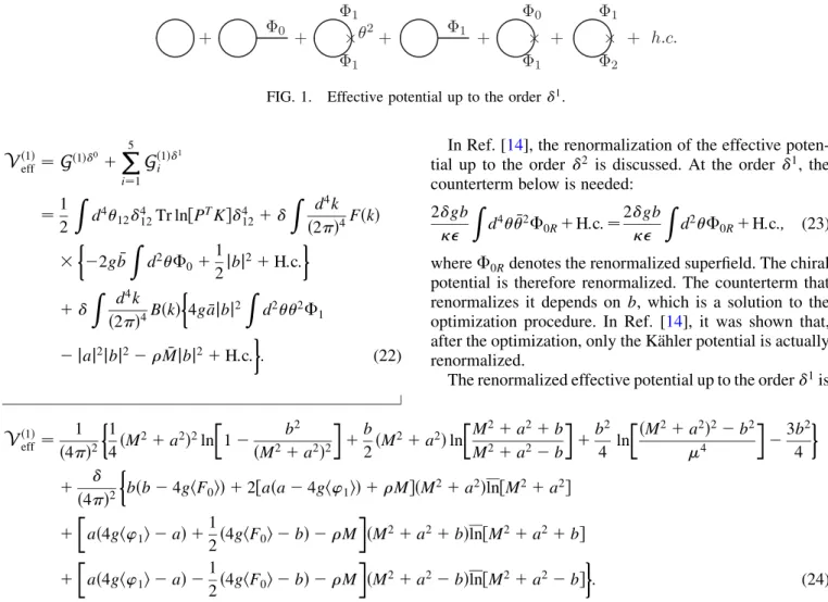
In Fig.1, we depict the diagrammatic sum of the effec-tive potential up to the order1 _(Vð1Þ

eff).

Notice that, because of the -dependent propagators, tadpole diagrams do not vanish any longer, as it usually happens in superspace. The first diagram is of order0_{, and}

we can see that it corresponds to the first term of the effective action, as given in (5). The third graph is a vacuum-type superdiagram with a quadratic insertion that stems from the2 _{component of theexpansion.}

With our super-Feynman rules and the results of Ref. [13], the effective potential up to the order 1 _reads

Vð1Þ

eff ¼G

ð1Þ0

þX

5

i¼1 Gð1Þ1

i

¼1

2

Z

d4

12412Tr ln½PTKŠ412þ Z d4k

ð2Þ4FðkÞ

2gbZ d2 0þ

1 2jbj

2_þH:c:

þZ d

4_k

ð2Þ4BðkÞ

4gajbj2Z _d22 1

jaj2_jbj2 _Mjbj2_þH:c:

: (22)

In Ref. [14], the renormalization of the effective poten-tial up to the order 2 _{is discussed. At the order}1_{, the}

counterterm below is needed: 2gbZ

d42

0RþH:c:¼ 2gbZ

d2

0RþH:c:; (23) where0Rdenotes the renormalized superfield. The chiral potential is therefore renormalized. The counterterm that renormalizes it depends on b, which is a solution to the optimization procedure. In Ref. [14], it was shown that, after the optimization, only the Ka¨hler potential is actually renormalized.

The renormalized effective potential up to the order1_is

Vð1Þ

eff ¼ 1

ð4Þ2 ₁

4ðM

2_þa2_Þ2_ln

1 b

2

ðM2_þa2_Þ2

þb

2ðM

2_þa2_Þln

_M2_þa2_þb

M2_þa2 _b

þb

2

4 ln

_ðM2_þa2_Þ2 _b2

4

_3b2

4

þ

ð4Þ2

bðb 4ghF0iÞ þ2½aða 4gh’1iÞ þMŠðM2þa2Þln½M2þa2Š

þ

að4gh’1i aÞ þ 1

2ð4ghF0i bÞ M

ðM2_þa2_þbÞln½M2_þa2_þbŠ

þ

að4gh’1i aÞ 1

2ð4ghF0i bÞ M

ðM2_þa2 _bÞln½M2_þa2 _bŠ

: (24)

For the time being, what we have is a perturbative result for the effective potential. To actually obtain a nonperturbative result, we apply the optimization procedure. We had to break the parametersM_ijinto-independent (a_ij) and-dependent (b_ij) parts and, with the help of (16), the optimized parameters turn out to be a₀₁¼a, b₁₁¼b, and ₁₂¼. Upon application of the PMS, to find the optimized parametersa,b, and, we have to solve the three coupled equations

@Vð1Þ

eff

@a

a¼a0

¼@V

ð1Þ

eff

@b

b¼b0

¼@V

ð1Þ

eff

@

¼0

¼0; (25)

at¼1, and plug the optimized valuesa₀,b₀, and₀ into (24). The following analytical solutions are encountered:

a₀ ¼4gh’₁i ¼a₀; b₀¼4ghF₀i ¼b₀; ₀ ¼0¼₀: (26)

The optimized parameters appear now as functions of the original coupling and fields, as expected. By plugging these results into (24), all the1 _{terms vanish and the optimized potential can be cast under the form below:}

Vð1Þ

eff¼G

ð1Þ0

¼ 1

ð8Þ2

ðm2_þ16g2_h’ 1i2Þ2ln

1 16g 2_hF

0i2

ðm2_þ16g2_h’ 1i2Þ2

þ8ghF0iðm2þ16g2h’1i2Þln

_m2_þ16g2_h’

1i2þ4ghF0i

m2_þ16g2_h’

1i2 4ghF0i

þ16g2_hF 0i2ln

_ðm2_þ16g2_h’

1i2Þ2 16g2hF0i2

4

48g2_hF 0i2

: (27)

The above result represents the Coleman-Weinberg–type potential [29,30] for the O’Raifeartaigh model [13,28], and it accounts for the sum of all one-loop diagrams. It is a nonperturbative result in that it takes into account all orders (actually infinite orders) in the original coupling constant.

III. EFFECTIVE POTENTIAL IN THE LDE ATOð2_Þ

We now present the order-2 _{results. At this order, we}

have one- and two-loop diagrams. Since the purpose of the present work is to be as clear as possible, the main part of this section is rather technical. All the results of this section are summarized in Sec.IV.

A. One Loop

To analyze the one-loop diagrams, we adopt the follow-ing strategy: there are 42 diagrams (plus some Hermitian conjugates), and we separate them in distinct sets; each diagram belonging to a certain set has the same propagator structure in the loop and differs from the other diagrams of the set only by the external classical superfields or by insertions ofa,b, or . Below, we show the expressions for these diagrams, set by set. We are going to use the notationJið;Þfor superspace integrals, which are listed in the Appendix.

The first set (Fig.2) is

Gð1Þ2

1 ¼42g2

Zd4_kd4 12

ð2Þ4 0ð1Þ0ð2Þ

₁

4D 2

1ðkÞh11i

₁

4D 2

2ð kÞh11i

þH:c:

¼4

2_g2

ð16Þ2b 2Z d

4_k

ð2Þ4FðkÞFðkÞJ1ð;Þ þH:c:

¼2

2_g2_hF 0i2

b ð

2_lnþ 2_{ln 2bÞ: (28)}

Gð1Þ2

2 ¼ 22gb

Zd4kd4₁₂

ð2Þ4 0ð1Þ 2 2

₁

4D 2

1ðkÞh11i

₁

4D 2

2ð kÞh11i

þH:c:

¼ 2

2_g

ð16Þ2bjbj

2Z d4k

ð2Þ4FðkÞFðkÞJ2ð;Þ þH:c:

¼

2_gbhF 0i

b ð

2_lnþ 2_{ln 2bÞ: (29)}

Gð1Þ2

3 ¼

1 4

2_b2Z d 4_kd4

12

ð2Þ4 2 122

₁

4D 2

1ðkÞh11i

₁

4D 2

2ð kÞh11i

þH:c:

¼

2

4ð16Þ2jbj 4Z d

4_k

ð2Þ4FðkÞFðkÞJ3ð;Þ þH:c:

¼

2_b2

8 bð

2_lnþ 2_{ln 2bÞ: (30)}

The second set (Fig.3) is

Gð1Þ2

4 ¼162g2

Zd4_kd4 12

ð2Þ4 0ð1Þ1ð2Þ

₁

4D 2

1ðkÞh11i

₁

4D 2

2ð kÞh01i

þH:c:

¼16

2_g2

ð16Þ2 ab Z d4k

ð2Þ4FðkÞfAðkÞJ4ð;Þ

jbj2_BðkÞJ

5ð;ÞgþH:c:

¼ 8

2_g2_ahF 0ih’1i

ðlnþ _{ln Þ: (31)}

Gð1Þ2

5 ¼ 42ga

Z d4kd4₁₂

ð2Þ4 0ð1Þ

₁

4D 2

1ðkÞh11i

₁

4D 2

2ð kÞh01i

þH:c:

¼ 4

2_g

ð16Þ2jaj

2_bZ d4k

ð2Þ4FðkÞfAðkÞJ6ð;Þ

jbj2_BðkÞJ

2ð;Þg þH:c:

¼2

2_ga2_hF 0i_ð

lnþ _{ln Þ:}

(32)

Gð1Þ2

6 ¼ 42gb

Z d4_kd4 12

ð2Þ4 1ð1Þ22

₁

4D 2 1ðkÞ

h11i

₁

4D 2

2ð kÞh10i

þH:c:

¼ 4

2_g

ð16Þ2ajbj

2Z d4k

ð2Þ4FðkÞfAðkÞJ7ð;Þ

jbj2_BðkÞJ

8ð;Þg þH:c:

¼2

2_gabh’ 1i

ðlnþ _{ln Þ: (33)}

Gð1Þ2

7 ¼2ab

Z d4_kd4 12

ð2Þ4 2 1

₁

4D 2

1ðkÞh11i

₁

4D 2

2ð kÞh01i

þH:c:

¼

2

ð16Þ2jaj

2_jbj2Z d 4_k

ð2Þ4FðkÞfAðkÞJ9ð;Þ

jbj2_BðkÞJ

3ð;Þg þH:c:

¼ a

2_b

2 ðln

þ _{ln Þ: (34)}

FIG. 2. DiagramsGð1Þ1 2,G ð1Þ2

2 , andG ð1Þ2

The third set (Fig.4) is

Gð1Þ2

8 ¼82g2

Zd4_kd4 12

ð2Þ4 1ð1Þ1ð2Þ

₁

4D 2

1ðkÞh11i

₁

4D 2

2ð kÞh00i

þH:c:

¼ 8

2_g2

ð16Þ2jaj

2_b2Z d4k

ð2Þ4FðkÞCðkÞJ10ð;Þ þH:c:

¼4

2_g2_a2_h’ 1i2

b ð

2_lnþ 2_{ln 2bÞ: (35)}

Gð1Þ2

9 ¼ 42ga

Z d4_kd4 12

ð2Þ4 1ð1Þ

₁

4D 2

1ðkÞh11i

₁

4D 2

2ð kÞh00i

þH:c:

¼4

2_g

ð16Þ2ajaj

2_b2Z d4k

ð2Þ4FðkÞCðkÞJ7ð;Þ þH:c:

¼ 2

2_ga3_h’ 1i

b ð

2_lnþ 2_{ln 2bÞ: (36)}

Gð1Þ2

10 ¼ 1 2

2_a2Zd4kd412

ð2Þ4

₁

4D 2

1ðkÞh11i

₁

4D 2

2ð kÞh00i

þH:c:

¼

2

2ð16Þ2a

2_jaj2_b2Z d 4_k

ð2Þ4FðkÞCðkÞJ9ð;Þ þH:c:

¼

2_a4

4 bð

2_lnþ 2_{ln 2bÞ: (37)}

The fourth set (Fig.5) is

Gð1Þ2

11 ¼82g2

Z d4_kd4 12

ð2Þ4 1ð1Þ1ð2Þ

₁

4D 2

1ðkÞh10i

₁

4D 2

2ð kÞh10i

þH:c:

¼8

2_g2

ð16Þ2 a 2Z d

4_k

ð2Þ4fAðkÞAðkÞJ11ð;Þ 2jbj2AðkÞBðkÞJ10ð;Þ þ jbj4BðkÞBðkÞJ12ð;Þg þH:c:

¼4

2_g2_a2_h’ 1i2

b

4bln2 _ð2_þ2bÞlnþ_{þ ð}2 _{2bÞln þ2b}

: (38)

Gð1Þ2

12 ¼ 42ga

Z d4_kd4 12

ð2Þ4 1ð1Þ

₁

4D 2

1ðkÞh10i

₁

4D 2

2ð kÞh10i

þH:c:

¼ 4

2_g

ð16Þ2jaj

2_aZ d4k

ð2Þ4fAðkÞAðkÞJ13ð;Þ 2jbj

2_{AðkÞBðkÞJ}

7ð;Þ þ jbj4BðkÞBðkÞJ8ð;Þg þH:c:

¼ 2

2_ga3_h’ 1i

b ½4bln

2 _ð2_þ2bÞlnþ_{þ ð}2 _{2bÞln þ2bŠ: (39)}

Gð1Þ2

13 ¼

1 2

2_a2Z d 4_kd4

12

ð2Þ4

₁

4D 2

1ðkÞh10i

₁

4D 2

2ð kÞh10i

þH:c:

¼

2

2ð16Þ2jaj 4Z d

4_k

ð2Þ4fAðkÞAðkÞJ14ð;Þ 2jbj2AðkÞBðkÞJ9ð;Þ þ jbj4BðkÞBðkÞJ3ð;Þg þH:c:

¼

2_a4

4 b

4bln2 _ð2_þ2bÞlnþ_{þ ð}2 _{2bÞln þ2b: (40)}

The fifth set (Fig.6) is

FIG. 4. DiagramsGð1Þ2

8 ,G ð1Þ2

9 , andG ð1Þ2

10 . FIG. 3. DiagramsGð1Þ4 2,G

ð1Þ2

5 ,G ð1Þ2

6 , andG ð1Þ2

Gð1Þ2

14 ¼82g2

Z d4_kd4 12

ð2Þ4 0ð1Þ0ð2Þ

₁

4D 2

1ðkÞh11i

₁

4D 2

2ð kÞh11i

¼8

2_g2

16

Z d4_k

ð2Þ4

EðkÞEðkÞJ15ð;Þ þ2

jbj2

16 EðkÞBðkÞJ16ð;Þ þ

jbj4

ð16Þ2BðkÞBðkÞJ17ð;Þ

¼8

2_g2_hF 0i21

ln

2

þ2

2_g2_hF 0i2

b ½4bln

2 _ð2_þ2bÞlnþ_{þ ð}2 _{2bÞln þ2bŠ: (41)}

Gð1Þ2

15 ¼ 22gb

Z d4_kd4 12

ð2Þ4 0ð1Þ 2 2

₁

4D 2

1ðkÞh11i

₁

4D 2

2ð kÞh11i

þH:c:

¼ 2

2_g

16 b

Z d4_k

ð2Þ4

EðkÞEðkÞJ18ð;Þ þ2

jbj2

16 EðkÞBðkÞJ2ð;Þ þ

jbj4

ð16Þ2BðkÞBðkÞJ19ð;Þ

þH:c:

¼ 4

2_gbhF 0i1

ln

2 2gbhF0i

b ½4bln

2 _ð2_þ2bÞlnþ_{þ ð}2 _{2bÞln þ2bŠ: (42)}

Gð1Þ2

16 ¼

1 2

2_jbj2Z d4kd412

ð2Þ4 2 122

₁

4D 2

1ðkÞh11i

₁

4D 2

2ð kÞh11i

¼

2

2ð16Þjbj

2Z d4k

ð2Þ4

EðkÞEðkÞJ20ð;Þ þ2

jbj2

16 EðkÞBðkÞJ3ð;Þ þ

jbj4

ð16Þ2BðkÞBðkÞJ21ð;Þ

¼

2_b2

2

₁

ln

2

þ

2_b2

8 b½4bln

2 _ð2_þ2bÞlnþ_{þ ð}2 _{2bÞln þ2bŠ: (43)}

The sixth set (Fig.7) is

Gð1Þ2

17 ¼162g2

Z d4_kd4 12

ð2Þ4 0ð1Þ1ð2Þ

₁

4D 2

1ðkÞh11i

₁

4D 2

2ð kÞh01i

þH:c:

¼16

2_g2

ð16Þ2 ab Z d4_k

ð2Þ4CðkÞ

EðkÞJ22ð;Þ þ

jbj2

16 BðkÞJ23ð;Þ

þH:c:

¼ 8

2_g2_ahF 0ih’1i_ð

lnþ _{ln Þ: (44)}

Gð1Þ2

18 ¼ 42ga

Z d4kd4₁₂

ð2Þ4 0ð1Þ

₁

4D 2

1ðkÞh11i

₁

4D 2

2ð kÞh01i

þH:c:

¼ 4

2_g

ð16Þ2jaj 2_bZ d

4_k

ð2Þ4CðkÞ

EðkÞJ6ð;Þ þ

jbj2

16 BðkÞJ24ð;Þ

þH:c:

¼2

2_ga2_hF 0i_ð

lnþ _{ln Þ: (45)}

Gð1Þ2

19 ¼ 42gb

Z d4_kd4 12

ð2Þ4 1ð1Þ22

₁

4D 2

1ðkÞh11i

₁

4D 2

2ð kÞh10i

þH:c:

¼ 4

2_g

ð16Þ2ajbj

2Z d4k

ð2Þ4CðkÞ

EðkÞJ25ð;Þ þ

jbj2

16 BðkÞJ26ð;Þ

þH:c:

¼2

2_gabh’ 1i

ðlnþ _{ln Þ: (46)}

FIG. 5. DiagramsGð1Þ112,G ð1Þ2

12 , andG ð1Þ2

13 . FIG. 6. DiagramsGð1Þ

2

14 ,G ð1Þ2

15 , andG ð1Þ2

Gð1Þ2

20 ¼2ab

Z d4_kd4 12

ð2Þ4 2 1

₁

4D 2

1ðkÞh11i

₁

4D 2

2ð kÞh01i

þH:c:

¼

2

ð16Þ2jaj

2_jbj2Z d 4_k

ð2Þ4CðkÞ

EðkÞJ9ð;Þ þ

jbj2

16 BðkÞJ27ð;Þ

þH:c:

¼

2_a2_b

2 ðln

þ _{ln Þ:}

(47) The seventh set (Fig.8) is

Gð1Þ2

21 ¼162g2

Z d4_kd4 12

ð2Þ4 1ð1Þ1ð2Þ

₁

4D 2

1ðkÞh11i

₁

4D 2

2ð kÞh00i

¼16

2_g2

16

Z d4_k

ð2Þ4

ðk2_{þ jMj}2_{ÞEðkÞAðkÞJ}

28ð;Þ þ jaj2jbj2EðkÞBðkÞJ29ð;Þ

þ ðk2_{þ jMj}2_Þjbj2

16 BðkÞAðkÞJ30ð;Þ þ

jaj2_jbj4

16 BðkÞBðkÞJ31ð;Þ

¼4

2_g2_h’ 1i2

b f4bð2

2 _M2_Þln2_{þ ½a}22_þ2þ_ðM2 þ_ފlnþ

½a22_{þ2 ðM}2 _{ފln 2bða}2_þ2M2 ₂2_Þ

: (48)

Gð1Þ2

22 ¼ 42ga

Z d4kd4₁₂

ð2Þ4 1ð1Þ

₁

4D 2

1ðkÞh11i

₁

4D 2

2ð kÞh00i

þH:c:

¼ 4

2_g

16 a

Z d4_k

ð2Þ4

ðk2_{þ jMj}2_{ÞEðkÞAðkÞJ}

13ð;Þ þ jaj2jbj2EðkÞBðkÞJ32ð;Þ þ ðk2þ jMj2Þ

jbj

2

16 BðkÞAðkÞJ7ð;Þ þ

jaj2_jbj4

16 BðkÞBðkÞJ8ð;Þ

þH:c:

¼ 2

2_gah’ 1i

b f4bð2

2 _M2_Þln2_{þ ½a}22_þ2þ_ðM2 þ_ފlnþ _½a22_{þ2 ðM}2 _ފln

2bða2_þ2M2 ₂2_{Þg: (49)}

Gð1Þ2

23 ¼2jaj2

Z d4_kd4 12

ð2Þ4

₁

4D 2

1ðkÞh11i

₁

4D 2

2ð kÞh00i

¼

2

16jaj

2Z d4k

ð2Þ4

ðk2_{þ jMj}2_{ÞEðkÞAðkÞJ}

33ð;Þ þ jaj2jbj2EðkÞBðkÞJ34ð;Þ þ ðk2þ jMj2Þ

jbj

2

16 BðkÞAðkÞJ35ð;Þ þ

jaj2_jbj4

16 BðkÞBðkÞJ36ð;Þ

¼

2_a2

4 bf4bð2

2 _M2_Þln2_{þ ½a}22_þ2þ_ðM2 þ_ފlnþ

½a22_{þ2 ðM}2 _{ފln 2bða}2_þ2M2 ₂2_{Þg: (50)}

FIG. 7. DiagramsGð1Þ172,G ð1Þ2

18 ,G ð1Þ2

19 , andG ð1Þ2

20 .

FIG. 8. DiagramsGð1Þ212,G ð1Þ2

22 , andG ð1Þ2

23 . FIG. 9. DiagramsG ð1Þ2

24 ,G ð1Þ2

25 , andG ð1Þ2

The eighth set (Fig.9) is

Gð1Þ2

24 ¼162g2

Zd4_kd4 12

ð2Þ4 1ð1Þ1ð2Þ

₁

4D 2

1ðkÞh10i

₁

4D 2

2ð kÞh10i

¼16

2_g2

ð16Þ3 jaj

2_jbj2Z d 4_k

ð2Þ4CðkÞCðkÞJ37ð;Þ

¼4

2_g2_a2_h’ 1i2

b ð

2_lnþ 2_{ln 2bÞ: (51)}

Gð1Þ2

25 ¼ 42ga

Zd4_kd4 12

ð2Þ4 1ð1Þ

₁

4D 2

1ðkÞh10i

₁

4D 2

2ð kÞh10i

þH:c:

¼ 4

2_g

ð16Þ3jaj

2_ajbj2Z d 4_k

ð2Þ4CðkÞCðkÞJ38ð;Þ þH:c:

¼ 2

2_ga3_h’ 1i

b ð

2_lnþ 2_{ln 2bÞ: (52)}

Gð1Þ2

26 ¼2jaj2

Z d4_kd4 12

ð2Þ4

₁

4D 2

1ðkÞh10i

₁

4D 2

2ð kÞh10i

¼

2

ð16Þ3jaj

4_jbj2Z d 4_k

ð2Þ4CðkÞCðkÞJ39ð;Þ

¼

2_a4

4 bð

2_lnþ 2_{ln 2bÞ: (53)}

The ninth set (Fig.10) is

Gð1Þ2

27 ¼ 42g

Z d4_kd4 12

ð2Þ4 0ð1Þ

₁

4D 2

1ðkÞh12i

₁

4D 2

2ð kÞh11i

þH:c:

¼ 4

2_g

ð16Þ2M b Z d4_k

ð2Þ4FðkÞfAðkÞJ6ð;Þ

jbj2_BðkÞJ

2ð;Þg þH:c:

¼2

2_gMhF 0i_ð

lnþ _{ln Þ: (54)}

Gð1Þ2

28 ¼2b

Z d4_kd4 12

ð2Þ4 2 1

₁

4D 2

1ðkÞh12i

₁

4D 2

2ð kÞh11i

þH:c:

¼

2

ð16Þ2Mjbj

2Z d4k

ð2Þ4FðkÞfAðkÞJ9ð;Þ

jbj2_BðkÞJ

3ð;Þg þH:c:

¼

2_Mb

2 ðln

þ _{ln Þ: (55)}

The tenth set (Fig.11) is

Gð1Þ2

29 ¼ 42g

Z d4kd4₁₂

ð2Þ4 1ð1Þ

₁

4D 2

1ðkÞh12i

₁

4D 2

2ð kÞh10i

þH:c:

¼ 4

2_g

ð16Þ2M a Z d4k

ð2Þ4fAðkÞAðkÞJ13ð;Þ 2jbj

2_{AðkÞBðkÞJ}

7ð;Þ þ jbj4BðkÞBðkÞJ8ð;Þg þH:c:

¼ 2

2_gMah’ 1i

b ½4bln

2 _ð2_þ2bÞlnþ_{þ ð}2 _{2bÞln þ2bŠ: (56)}

Gð1Þ2

30 ¼2a

Z d4kd4₁₂

ð2Þ4

₁

4D 2

1ðkÞh12i

₁

4D 2

2ð kÞh10i

þH:c:

¼

2

ð16Þ2Mjaj 2Z d

4_k

ð2Þ4fAðkÞAðkÞJ14ð;Þ 2jbj2AðkÞBðkÞJ9ð;Þ þ jbj4BðkÞBðkÞJ36ð;Þg þH:c:

¼

2_Ma2

2 b ½4bln

2 _ð2_þ2bÞlnþ_{þ ð}2 _{2bÞln þ2bŠ: (57)}

The eleventh set (Fig.12) is

FIG. 10. DiagramsGð1Þ2

27 andG ð1Þ2

Gð1Þ2

31 ¼ 42g

Z d4_kd4 12

ð2Þ4 1ð1Þ

₁

4D 2

1ðkÞh11i

₁

4D 2

2ð kÞh20i

þH:c:

¼4

2_g

ð16Þ2M ab 2Z d

4_k

ð2Þ4FðkÞCðkÞJ7ð;Þ þH:c:

¼ 2

2_gMah’ 1i

b ð

2_lnþ 2_{ln 2bÞ: (58)}

Gð1Þ2

32 ¼2a

Z d4_kd4 12

ð2Þ4

₁

4D 2

1ðkÞh11i

₁

4D 2

2ð kÞh20i

þH:c:

¼

2

ð16Þ2Mjaj

2_b2Z d4k

ð2Þ4FðkÞCðkÞJ9ð;Þ þH:c:

¼

2_Ma2

2 b ð

2_lnþ 2_{ln 2bÞ: (59)}

The twelfth set (Fig.13) is

Gð1Þ2

33 ¼ 42g

Z d4_kd4 12

ð2Þ4 0ð1Þ

₁

4D 2

1ðkÞh12i

₁

4D 2

2ð kÞh11i

þH:c:

¼4

2_g

16 M b

Z d4_k

ð2Þ4FðkÞ

EðkÞJ18ð;Þ þ

jbj2

16 BðkÞJ2ð;Þ

þH:c:

¼2

2_gMhF 0i

ðlnþ _{ln Þ: (60)}

Gð1Þ2

34 ¼2b

Z d4kd4₁₂

ð2Þ4 2 1

₁

4D 2

1ðkÞh12i

₁

4D 2

2ð kÞh11i

þH:c:

¼

2

16M jbj 2Z d

4_k

ð2Þ4FðkÞ

EðkÞJ20ð;Þ þ

jbj2

16 BðkÞJ36ð;Þ

þH:c:

¼

2_Mb

2 ðln

þ _{ln Þ: (61)}

The thirteenth set (Fig.14) is

Gð1Þ2

35 ¼ 42g

Z d4_kd4 12

ð2Þ4 1ð1Þ

₁

4D 2

1ðkÞh12i

₁

4D 2

2ð kÞh10i

þH:c:

¼4

2_g

ð16Þ2M ajbj 2Z d

4_k

ð2Þ4FðkÞCðkÞJ7ð;Þ þH:c:

¼ 2

2_gMah’ 1i

b ð

2_lnþ 2_{ln 2bÞ: (62)}

Gð1Þ2

36 ¼2a

Z d4kd4₁₂

ð2Þ4

₁

4D 2

1ðkÞh12i

₁

4D 2

2ð kÞh10i

þH:c:

¼

2

ð16Þ2M jaj

2_jbj2Z d 4_k

ð2Þ4FðkÞCðkÞJ9ð;Þ þH:c:

¼

2_Ma2

2 b ð

2_lnþ 2_{ln 2bÞ: (63)}

FIG. 12. DiagramsGð1Þ312 andG ð1Þ2

32 . FIG. 11. DiagramsGð1Þ292 andG

ð1Þ2

30 . FIG. 13. DiagramsGð1Þ

2

33 andG ð1Þ2

34 .

The fourteenth set (Fig.15) is

Gð1Þ2

37 ¼ 42g

Z d4_kd4 12

ð2Þ4 1ð1Þ

₁

4D 2

1ðkÞh11i

₁

4D 2

2ð kÞh20i

þH:c:

¼ 4

2_g

16 M a

Z d4_k

ð2Þ4

EðkÞAðkÞJ40ð;Þ þ jbj2EðkÞBðkÞJ32ð;Þ

jbj2

16 BðkÞAðkÞJ7ð;Þ þ

jbj4

16 BðkÞBðkÞJ8ð;Þ

þH:c:

¼ 2

2_gMah’ 1i

b ½4bln

2 _ð2_þ2bÞlnþ_{þ ð}2 _{2bÞln þ2bŠ: (64)}

Gð1Þ2

38 ¼2a

Z d4_kd4 12

ð2Þ4

₁

4D 2

1ðkÞh11i

₁

4D 2

2ð kÞh20i

þH:c:

¼

2

16M jaj

2Z d4k

ð2Þ4

EðkÞAðkÞJ33ð;Þ þ jbj2EðkÞBðkÞJ34ð;Þ

jbj2

16 BðkÞAðkÞJ35ð;Þ þ

jbj4

16 BðkÞBðkÞJ36ð;Þ

þH:c:

¼

2_Ma2

2 b ½4bln

2 _ð2_þ2bÞlnþ_{þ ð}2 _{2bÞln þ2bŠ: (65)}

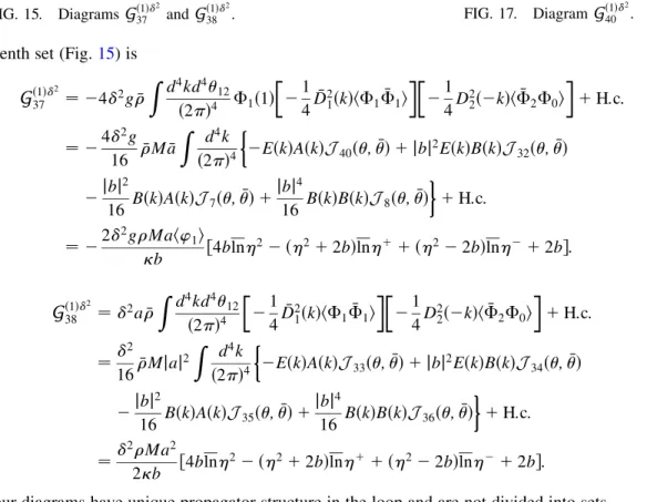
The last four diagrams have unique propagator structure in the loop and are not divided into sets. The thirty-ninth diagram (Fig.16) is

Gð1Þ2

39 ¼

1 2

22Z d4kd412

ð2Þ4

₁

4D 2

1ðkÞh22i

₁

4D 2

2ð kÞh11i

þH:c:

¼

2

2ð16Þ2

2_jMj2_b2Z d4k

ð2Þ4CðkÞFðkÞJ9ð;Þ þH:c:

¼

22_M2

4 b ð

2_lnþ 2_{ln 2bÞ: (66)}

The fortieth diagram (Fig.17) is

Gð1Þ2

40 ¼2jj2

Zd4_kd4 12

ð2Þ4

₁

4D 2

1ðkÞh22i

₁

4D 2

2ð kÞh11i

¼

2

16jj 2Z d

4_k

ð2Þ4

ðk2_{þ jaj}2_{ÞAðkÞEðkÞJ}

33ð;Þ þ ðk2þ jaj2Þ

jbj2

16AðkÞBðkÞJ35ð;Þ

þ jMj2_jbj2_{BðkÞEðkÞJ}

34ð;Þ þ

jMj2_jbj4

16 BðkÞBðkÞJ36ð;Þ

¼

22

4 bf4bð2

2 _a2_Þln2 _½2þ_ðþ _a2_{Þ M}22_Šlnþ

þ ½2 ð a2_{Þ M}22_{Šln þ2bð2}2 _2a2 _M2_{Þg: (67)}

FIG. 15. DiagramsGð1Þ2

37 andG ð1Þ2

38 .

FIG. 16. DiagramGð1Þ392.

FIG. 17. DiagramGð1Þ2

40 .

The forty-first diagram (Fig.18) is

Gð1Þ2

41 ¼

1 2

22Z d 4_kd4

12

ð2Þ4

₁

4D 2

1ðkÞh21i

₁

4D 2

2ð kÞh21i

þH:c:

¼

2

2ð16Þ2

2_M2Z d 4_k

ð2Þ4fAðkÞAðkÞJ14ð;Þ 2jbj

2_{AðkÞBðkÞJ}

9ð;Þ þ jbj4BðkÞBðkÞJ3ð;Þg þH:c:

¼

22_M2

4 b ½4bln

2 _ð2_þ2bÞlnþ_{þ ð}2 _{2bÞln þ2bŠ: (68)}

Finally, the forty-second diagram (Fig.19) is

Gð1Þ2

42 ¼2jj2

Z d4kd4₁₂

ð2Þ4

₁

4D 2

1ðkÞh21i

₁

4D 2

2ð kÞh21i

¼

2

16jj

2_jMj2_jbj2Z d 4_k

ð2Þ4FðkÞFðkÞJ20ð;Þ

¼

22_M2

4 b ð

2_lnþ 2_{ln 2bÞ: (69)}

The diagrams Gð₁₄1Þ2, G₁₅ð1Þ2, andGð₁₆1Þ2 of the fifth set give divergent contributions, and we will discuss their renormalization later.

B. Two Loops

The two-loop diagrams are shown in Fig.20.

To calculate the two-loop diagrams, we use the tech-nique developed in Ref. [31]. The contribution of the first diagram is given by

Gð2Þ2

1 ¼42g2

Zd4_pd4_kd4 12

ð2Þ8

₁

4D 2

1ðpÞh00i

₁

4D 2

2ðkÞh11i

₁

16D 2

1ðqÞD22ð qÞh11i

¼

2_g2

ð16Þ3a 2_b3Z d

4_pd4_k

ð2Þ8 CðpÞFðkÞFðqÞI1ð;Þ;

(70) withq¼ ðk pÞ, and the integralI1ð;Þis given in the

Appendix. PluggingI1ð;Þinto (70), we obtain

Gð2Þ2

1 ¼ 42g2a2b3

Z d4_pd4_k

ð2Þ8 CðpÞFðkÞFðqÞp

2_{: (71)}

To handle with the integral above and the other mo-mentum space integrals that will appear in the following, we have adopted the following strategy: for each of them, we split the integrand with the help of the method of partial fraction decomposition and write each integral as the sum of other integrals with just three terms in the denominator. The remaining integrals are well known in the literature, and we use the results of Refs. [32–34] to compute them.

From now on, we define 2_¼m2_þa2_,

_¼m2_þa2_{b and adopt the same notation of}

Refs. [32–34] for the integrals Iðx; y; zÞ, Jðx; yÞ, andJðxÞ:

JðxÞ ¼ x

þxðlnx 1Þ; (72)

2_{Jðx; yÞ ¼xy 1}

2þ

1

ð2 lnx lnyÞ

þ ð1 lnx lnyþlnxlnyÞ

; (73)

2_{Iðx; y; zÞ ¼} c 22

1

_3c

2 L1

₁

2fL2 6L1

þ ðyþz xÞlnylnzþ ðzþx yÞlnzlnx

þ ðyþx zÞlnylnxþðx; y; zÞ

þc½7þð2ފg; (74)

where FIG. 19. DiagramGð1Þ2

42 .

¼ ð4Þ2_;

c¼xþyþz;

lnX¼ln

_X

2

þ ln4;

L_m¼xlnmxþylnmyþzlnmz;

ðx; y; zÞ ¼S

2 lnzþx y S 2z ln

zþy x S

2z ln

x zln

y

z 2 Li2

_{zþx y S}

2z

2 Li2

_{zþy x S}

2z

þ

2

3

;

S¼qffiffiffiffiffiffiffiffiffiffiffiffiffiffiffiffiffiffiffiffiffiffiffiffiffiffiffiffiffiffiffiffiffiffiffiffiffiffiffiffiffiffiffiffiffiffiffiffiffiffiffiffiffiffiffiffiffiffiffiffiffiffiffiffiffiffiffiffix2_þy2_þz2 _{2xy 2yz 2zx;}

Li2ðzÞ ¼ Zz

0

lnð1 tÞ

t dtðdilogarithm functionÞ:

So, the total contribution of the first two-loop diagram is

Gð2Þ2

1 ¼

2_g2_a2 2 ½Ið

þ_; þ_; þ_{Þ 3Ið}þ_; þ_{; Þ þ3Ið}þ_{; ; Þ Ið ; ; ފ: (75)}

The contribution of the second diagram is given by

Gð2Þ2

2 ¼82g2

Z d4_pd4_kd4 12

ð2Þ8

₁

4D 2

1ðpÞh01i

₁

4D 2

2ðkÞh01i

₁

16D 2

1ðqÞD22ð qÞh11i

¼2

2_g2

ð16Þ3 a 2_bZ d

4_pd4_k

ð2Þ8 fAðpÞAðkÞFðqÞI2ð;Þ 2b2AðpÞBðkÞFðqÞI3ð;Þ þb4BðpÞBðkÞFðqÞI4ð;Þg: (76)

PluggingI2ð;Þ,I3ð;Þ, andI4ð;Þinto (76), we obtain

Gð2Þ2

2 ¼ 82g2a2b3

2Z d 4_pd4_k

ð2Þ8 AðpÞBðkÞFðqÞp

2_þb2Z d 4_pd4_k

ð2Þ8 BðpÞBðkÞFðqÞ

: (77)

Decomposing the momentum space integrals, we get the contribution

Gð2Þ2

2 ¼2g2a2½ 4Ið2; 2;

þ_{Þ þ4Ið}2_; 2_{; Þ þIð}þ_; þ_; þ_{Þ þIð}þ_; þ_{; Þ}

Iðþ; ; Þ Ið ; ; ފ: (78)

The contribution of the third diagram is given by

Gð2Þ2

3 ¼162g2

Zd4_pd4_kd4 12

ð2Þ8

₁

4D 2

1ðpÞh10i

₁

4D 2

2ðkÞh11i

₁

16D 2

1ðqÞD22ð qÞh01i

¼

2_g2

ð16Þ3a 2_b2Z d

4_pd4_k

ð2Þ8 CðpÞCðqÞ

EðkÞI5ð;Þ þ 1

16b

2_{BðkÞI6ð;Þ}

: (79)

PluggingI5ð;ÞandI6ð;Þinto (79), we obtain

Gð2Þ2

3 ¼162g2a2b2

Z d4_pd4_k

ð2Þ8 CðpÞEðkÞCðqÞp

2_q2_þb2Z d 4_pd4_k

ð2Þ8 CðpÞBðkÞCðqÞp 2_q2

: (80)

Decomposing the momentum space integrals, we have

Gð2Þ2

3 ¼22g2a2½Iðþ; þ; þÞ Iðþ; þ; Þ Iðþ; ; Þ þIð ; ; ފ: (81)

¼8

2_g2

ð16Þ2a 2_b2Zd

4_pd4_k

ð2Þ8 BðqÞ

EðpÞEðkÞI7ð;Þþ 1 8b

2_{EðpÞBðkÞI}

8ð;Þþ 1

ð16Þ2b

4_{BðpÞBðkÞI} 9ð;Þ

þ8

2_g2

ð16Þ2

Zd4_pd4_k

ð2Þ8 AðqÞðq 2_þm2_Þ

EðpÞEðkÞI10ð;Þþ 1 8b

2_{EðpÞBðkÞI}

11ð;Þþ 1

ð16Þ2b

4_{BðpÞBðkÞI} 12ð;Þ

: (82)

PluggingI7ð;Þ–I12ð;Þinto (82), we get Gð2Þ2

4 ¼82g2b2

a2Z d 4_pd4_k

ð2Þ8 EðpÞEðkÞBðqÞ þ2a 2_b2Z d

4_pd4_k

ð2Þ8 EðpÞBðkÞBðqÞ

þa2_b4Z d 4_pd4_k

ð2Þ8 BðpÞBðkÞBðqÞ 2

Z d4_pd4_k

ð2Þ8 EðpÞBðkÞAðqÞk

2_q2 _b2Z d 4_pd4_k

ð2Þ8 BðpÞBðkÞAðqÞq 4

2m2Z d 4_pd4_k

ð2Þ8 EðpÞBðkÞAðqÞk

2 _m2_b2Z d 4_pd4_k

ð2Þ8 BðpÞBðkÞAðqÞq 2

: (83)

Decomposing the momentum space integrals, we obtain the total contribution of the fourth diagram:

Gð2Þ2

4 ¼2g2

8a2

Ið2_; 2_; 2_{Þ þ} b

2Ið

2_; 2_; þ_Þ b 2Ið

2_; 2_{; Þ}

þ8m2

2Ið2_; 2_{;0Þ þ}

þ

2 Ið

2_; þ_;0Þ

þ

2 Ið

2_{; ;0Þ}

þa2_½Iðþ_; þ_; þ_{Þ þ3Ið}þ_; þ_{; Þ þ3Ið}þ_{; ; Þ þIð ; ; ފ}

þ2½ 4Jð2_; 2_{Þ þ4Jð}2_; þ_{Þ þ4Jð}2_{; Þ Jð}þ_; þ_{Þ 2Jð}þ_{; Þ Jð ; ފ: (84)}

Unlike the first three two-loop diagrams, Gð2Þ2

4 gives a

divergent contribution; however, its renormalization is trivial, since it is a vacuum diagram.

C. Regularization and renormalization

The divergent diagrams of order2 _are Gð1Þ2

14 ¼

₈2_g2₁

ln

2

þ2

2_g2

b ½4bln

2 _ð2_þ2bÞlnþ

þð2 _{2bÞln þ2bŠ}Z_d4

00; (85)

Gð1Þ2

15 ¼

₂2_gb1

ln

2

2_gb

2 b ½4bln

2

ð2_þ2bÞlnþ_{þ ð}2 _{2bÞln þ2bŠ}

Z d42

0þH:c:; (86)

Gð1Þ2

16 ¼ 2_b2

2

₁

ln

2

þ

2_b2

8 b½4bln

2 _ð2_þ2bÞlnþ

þ ð2 _{2bÞln þ2bŠ} Z_d422_{: (87)}

The diagramGð₁₆1Þ2 is a vacuum diagram, and thus its renormalization is trivial. To renormalize the divergent term inGð₁₄1Þ2, we introduce the counterterm

82_g2 _Z

d4

0R0R; (88) and, for the divergent term in Gð₁₅1Þ2, we introduce the counterterm

22_gb Z

d42

0RþH:c:¼

22_gbZ

d2

0RþH:c:

(89) As mentioned in the previous section and shown in Ref. [14], plugging the solution for the optimized parame-ter bin (89), only the Ka¨hler potential is actually renor-malized, in agreement with the nonrenormalization theorem.

IV. SUMMARY OF THE RESULTS AND NUMERICAL ANALYSIS

In this last section we summarize the perturbative results for the effective potential up to the order 2_{. We}

also derive nonperturbative corrections to the effective potential by implementing the PMS criterion numerically. Up to this order, the renormalized effective potential can be written as

Veff ¼Vtreeeff þV

0

effþV

1

effþV

2

eff: (90)

The tree level potential is given by

Vtree

eff ¼Vð’1Þ ¼ ðþg’12Þ2þm2’21; (91)

with <0.

The vacuum diagram of order0 _is V0

eff ¼ 1

ð4Þ2 ₁

4ðM

2_þa2_Þ2_ln

1 b

2

ðM2_þa2_Þ2

þb

2ðM

2_þa2_Þln

_M2_þa2_þb

M2_þa2 _b

þb

2

4 ln

_ðM2_þa2_Þ2 _b2

4

_3b2

4

:

(92) The one-loop contribution for the effective potential atOð1_{Þis given by}

V1

eff ¼

ð4Þ2

bðb 4ghF0iÞ þ2½aða 4gh’1iÞ þMŠðM2þa2Þln½M2þa2Š

þ

að4gh’1i aÞ þ 1

2ð4ghF0i bÞ M

ðM2_þa2_þbÞln½M2_þa2_þbŠ

þ

að4gh’1i aÞ 1

2ð4ghF0i bÞ M

ðM2_þa2 _bÞln½M2_þa2 _{bŠ: (93)}

AtOð2_{Þ, we separate the contributions of one- and two-loop diagrams:} V2

eff ¼V

2

effðIÞþV 2

effðIIÞ; (94)

where

V2

effðIÞ¼ 2

ð4Þ2

½ða 4gh’₁iÞ2_ðM2_þ3a2_{Þ þaMða 4gh’}

1iÞ þ2ð3M2þa2ފlnðM2þa2Þ

1 2

ða 4gh’1iÞ½ða 4gh’1iÞðM2þ3a2þbÞ þ2aðb 4ghF0iÞ þ4aMŠ

þ1

2ðb 4ghF0iÞ½ðb 4ghF0iÞ þ4MŠ þ

2_ð3M2_þa2_þbÞlnðM2_þa2_þbÞ

1 2

ða 4gh’1iÞ½ða 4gh’1iÞðM2þ3a2 bÞ 2aðb 4ghF0iÞ þ4aMŠ

þ1

2ðb 4ghF0iÞ½ðb 4ghF0iÞ 4MŠ þ

2_ð3M2_þa2 _bÞ

lnðM2_þa2 _bÞ

; (95)

and

V2

effðIIÞ¼ 2_g2

ð4Þ4

₄

ðM2_þa2_Þ½4ðM

2_þa2_Þ3_þbðM2_þa2 _bÞðM2 _2a2_ފln2_ðM2_þa2_Þ ðM2þa2þbÞ

ðM2_þa2_Þ ½ðM 2_þa2_Þ

ð6M2_þ17a2_{Þ þ2bðM}2_þ3a2_ފln2_ðM2_þa2_{þbÞ 3ðM}2_þa2 _bÞð2M2_þ3a2 _2bÞln2_ðM2_þa2 _bÞ

þ8ðM2_þa2_þbÞð2a2 _bÞlnðM2_þa2_ÞlnðM2_þa2_{þbÞ þ}8a2bðM2þa2 bÞ

ðM2_þa2_Þ lnðM

2_þa2_ÞlnðM2_þa2 _bÞ

2ðM2_þa2_þbÞð2M2_þ3a2 _2bÞlnðM2_þa2_þbÞlnðM2_þa2 _{bÞ þ} 8M2b

ðM2_þa2_Þ

bln

_ðM2_þa2_Þ2

ðM2_þa2_Þ2 _b2

ðM2_þa2_ÞlnM2þa2þb

M2_þa2 _b

lnb 24ðM2_þa2_Þð2M2_þ3a2_ÞlnðM2_þa2_{Þ þ12ðM}2_þa2_þbÞð2M2_þ3a2_þ2bÞ

lnðM2_þa2_{þbÞ þ12ðM}2_þa2 _bÞð2M2_þ3a2 _2bÞlnðM2_þa2 _{bÞ þa}2_½4ðM2_þa2_;M2_þa2_;M2_þa2_Þ

3ðM2_þa2_þb;M2_þa2_þb;M2_þa2_{þbÞ ðM}2_þa2_þb;M2_þa2 _b;M2_þa2 _bފ

þ4a

2_ðM2_þa2 _bÞ

ðM2_þa2_Þ ½ðM

2_þa2_;M2_þa2_;M2_þa2_{þbÞ ðM}2_þa2_;M2_þa2_;M2_þa2 _{bފ þ} 8M 2_b

ðM2_þa2_Þ

ðM2_þa2_þbÞLi 2

_M2_þa2

M2_þa2_þb

þ ðM2_þa2 _bÞLi 2

_M2_þa2 _b

M2_þa2

56b2 4 3b

2_ð2M2_þbÞ

: (96)