Galerkin-Method Approach to Nonlinear Soliton Classical Stability
C. A. Linhares and H. P. de Oliveira
Departamento de F´ısica Te´orica - Instituto de F´ısica A. D. Tavares Universidade do Estado do Rio de Janeiro
CEP 20550-013 Rio de Janeiro – RJ, Brazil
Received on 4 December, 2006
We examine the evolution of perturbations on the kink configuration inλφ4theory and of the Nielsen–Olesen vortex in scalar electrodynamics through the Galerkin method. The problem is reduced to a finite dynamical system for which the linear and nonlinear regimes are studied. The linear stability of both is associated to a motion in a stable torus present in phase space, whereas the nonlinear evolution of perturbations can be viewed as a consequence of the breakdown of the tori structure and the onset of chaos. We discuss this regime in connection with the stability of the configurations. Also, the Galerkin method is used to obtain approximate analytical expressions for the vortex profile.
Keywords: Stability of solitons; Nielsen-Olesen vortex; Galerkin model
I. INTRODUCTION
One of the main features of soliton (solitary wave) solutions of nonlinear differential equations is the permanence of its shape in time. Besides this formal and important aspect, soli-tonic configurations are present in many areas of physics, be-sides the original one in hydrodynamics [1]. For instance, we may cite in elementary particle physics where solitons may be regarded as extended particlelike solutions of nonlinear field equations of various types, providing well-known configura-tions such as the kink solution inφ4or sine–Gordon theory, or as vortices and monopoles in gauge field theories [2]. In cosmology, extended configurations like cosmic strings and domain walls are considered as possible candidates of dark matter [3]. Importantly, also, in condensed-matter physics, solitons may appear as fluxons present in the Josephson junc-tion transmission line [4]. Many other examples are studied in the literature.
Much attention has been given to the study of the behav-ior of solitons under the influence of some perturbations, in which the very first approach was focused on linear perturba-tion theory [2],[5]-[9]. Physically, such perturbaperturba-tions repre-sent the interaction between the soliton with very small spa-tial inhomogeneities which, in the case of condensed matter, may be thought of as impurities or defects typical even in the purest material samples. On the other hand, it can happen that the spatial inhomogeneities are not restricted to be small, and therefore the problem of their interaction with solitary waves naturally emerges. In this situation, the basic difficulty is the inner complexity of the problem due to the high degree of non-linearity present even in the most simple differential equations of interest. Therefore, most analysis on soliton stability relied entirely on numerical methods or were restricted to the linear order of perturbation theory.
Nonlinearities are also the main reason for the impossi-bility of determining analytical expressions for the functions which define solitonic configurations of field theories in more than one spatial dimensions, such as vortices in gauge theo-ries, even in the static case. These are again obtained usu-ally through numerical calculations, and these seem to be
in-evitable for the discussion of stability of these configurations under small perturbations.
Our purpose in the present article is to approach the subject so that the contributions from nonlinear terms in the differ-ential equations are more explicitly controlled. To this end, we apply the so-called ‘traditional Galerkin method’ [10, 11], of wide applications to nonlinear problems encountered, for instance, in the physics and engineering of dynamical fluids (for a recent reference see [12]). Although it provides only approximate solutions to the differential equation one wishes to study, and in the end one needs to resort to numerical cal-culations, the method is able to produce some more analytical information on the problem, and in a few situations it may be completely solved by a symbol-manipulating computer lan-guage.
The Galerkin method starts by postulating a solution in spacetime to a partial differential equation in the form of a finite series of an arbitrary set of space-dependent functions, which are chosen to suit the boundary conditions of the prob-lem, multiplied by time-dependent coefficients. By inserting this trial solution into the differential equation and projecting onto the same set of functions, one gets a system of ordinary differential equations in time for the series coefficients. This last system is then solved numerically, providing the time evo-lution of the coefficients. In the simpler static case, the co-efficients are just numbers, and the last system to solve is an algebraic one. In both situations, the numberNof terms in the series is however also arbitrary, and it must be decided upon according to the desired numerical accuracy. This defines a truncation of a possibly infinite series, which is then differ-ently approximated for different choices ofN. One expects that for growingN the approximation converges to the true solution, and this feature is illustrated below for the specific problems we study.
and space.
In this paper we apply the approach outlined above to topo-logical configurations appearing in two relativistic classical field theories. It is organized as follows. In Section 2, we con-sider the topological kink found in (1+1)-dimensional scalar field theory with quartic potential in the broken-symmetric phase. We study its stability by adding to it a general pertur-bation function in spacetime with an initial Gaussian shape. The perturbation is then made to evolve according to the field equation of the theory (sometimes called the ‘nonlin-ear Klein–Gordon equation’), of which we keep all nonlin‘nonlin-ear terms, and treat it following the Galerkin prescription. The analysis of the results we have obtained from the numerical integration of the system of ordinary differential equations for Galerkin coefficients then ensues. We also exhibit there the power spectrum of the perturbed field, for which an average over the space coordinates is taken, showing the typical fea-tures of a transition to a chaotic behavior. In Section 3, we turn first to the Nielsen–Olesen static vortex configuration of scalar electrodynamics, which may play a role in the descrip-tion of superconducting phase transidescrip-tions [15] or even in cos-mic strings scenarios [16]. As far as we know, there is still lacking in the literature a closed analytical expression for it. Thus, before tackling the study of vortex perturbations, we had here to establish the two radial functions on a plane satis-fying a system of coupled nonlinear partial differential equa-tions of which the vortex is a solution. We are able to solve completely the Galerkin algebraic system, providing expres-sions, for each value of the topological charge, of the func-tions which define the vortex shape. The question of the vor-tex stability under time-dependent perturbations of these func-tions is studied next. Finally, in the last Section we conclude. In the Appendix we present a few Galerkin-constructed static Nielsen–Olesen vortices for varying characteristic parameters and topological numbers.
II. NONLINEAR PERTURBATIONS OF THE KINK SOLUTION
A. Basic Galerkin approach to the kink and its perturbations
We here consider the evolution of perturbations of the usual kink solution of a real scalar field theory with potential
V(φ) =1
4 ¡
φ2−b2¢2
in (1+1)-dimensional spacetime, where bis a constant which parametrizes the spontaneous symmetry breakdown. The field equation for that theory in reads
µ∂2 ∂t2−
∂2 ∂x2
φ(x,t) +³φ(x,t)2−b2´φ(x,t) =0. (1)
Its (static) kink solution has the form φ0(x) =btanh
b
√
2x, (2)
where the space coordinatexruns from−∞to+∞. We study the behavior of general perturbations of this kink solution by
writing
φ(x,t) =φ0(x) +δφ(x,t). (3) For the sake of convenience, we introduce a new spatial vari-ableξ≡tanh³bx/√2´, so that the interval −∞<x<+∞ corresponds to−1<ξ<1 and the unperturbed kink is now described asφ0(ξ) =bξ. After rewriting the field equation (1) for theξvariable, we introduce Eq. (3) onto it, and obtain a differential equation for the perturbationδφ(x,t):
(δφ)..−b
2 2(1−ξ
2)£¡
1−ξ2¢
(δφ)′′−2ξ(δφ)′¤
+¡
3ξ2
−1¢b2δφ+ (3bξ+δφ) (δφ)2=0, (4) where the prime means derivative with respect toξ. If one wishes to restrict the problem to linear perturbations, it is then necessary to drop the last term in the lhs of Eq. (4). A com-plete analysis of this case can be found in Ref. [7].
We seek instead solutions to the complete equation (4), for which we implement the Galerkin procedure [10]. Also, we adopt the following boundary conditions[7] to be satisfied by the perturbationδφ:
δφ(ξ=±1,t) =0, (5) which is equivalent to δφ(x=±∞,t) =0. The Galerkin method postulates an approximate solution (the ‘trial’ solu-tion) for the equation as a finite sum, which in our case the perturbationδφmay be written
δφ(ξ,t) =
N
∑
k=0
ak(t)ψk(ξ), (6)
where theψk constitute a set of analytic basis functions, to
be chosen suitably, as a generalization of a Fourier expansion, andNis the order of the series truncation. It remains therefore to compute theN+1 ‘modal’ coefficientsak(t).
Our choice of basis functions, which satisfy the boundary conditions, is
ψk(ξ) =Tk+2(ξ)−Tk(ξ), (7)
whereTk(ξ)is the Chebyshev polynomial of degreek.
Prop-erties of Chebyshev polynomials are well-known (see, for in-stance, [17]); the main one for our purposes is that they are orthogonal in the interval(−1,1)over a weight(1−ξ2)−1/2.
The behavior of the modal coefficients ak(t)are dictated
by the equations resulting from the following steps: (i) intro-duce the decomposition (6) into the lhs of Eq. (4), so that it produces an expression known by the residual equation, Res(ξ,t)≃0, for which the equality is attained only for the exact solution (N→∞); (ii) project the residual equation onto each modeψj(ξ), for all j=0, . . . ,N, through the operation
Res,ψj®≡R−11dξRes(ξ,t)ψj. The Galerkin method
estab-lishes that each projection must vanish, i. e., R,ψj
®
the second-order time derivatives (this is necessary since the basis functionsψk(ξ)are not orthogonal), it follows that
¨ a0(t) +5
2a0(t) 3+b2
2a2(t) +
23595b2 7429 a10(t)
+···=0 ¨
a1(t) + 3b2
2 a1(t) +
44987b2
63365 a11(t) +···=0 ¨
a2(t) +11b 2 4 a2(t)−
3b2 4 a4(t) +
16335b2 1748 a10(t)
+···=0 ..
. ¨ a11(t)−
63b2 4 a9(t) +
3701b2
58 a11(t) +···=0, for theN=11 case. Since each of the above equations has typically more than 200 terms (a number which grows for in-creasingN), with all kinds of square and cubic combinations of the modal coefficients, we have just displayed the linear terms, except for the cubic term in the first equation. As a mat-ter of fact, it is possible to envisage the behavior of the linear perturbations in a very simple way, as well as to give an ac-count of the effect of the nonlinearities for a more general per-turbation using our dynamical system approach. For instance, in the case of linearized perturbations the set of equations for a1(t),a2(t), ..,aN(t)are reduced to coupled harmonic
oscilla-tors for which there is no contribution froma0(t). Then, once theak(t),k=1,2, ...,N, are known, the evolution ofa0(t)is then determined. It should be noticed that in all equations, including the one for ¨a0(t), the linear term ina0 is lacking. This peculiar aspect of the linearized equations is a conse-quence of the existence of a static configuration characterized bya0=const.,a1=a2=...=aN=0, as we are going to see.
In order to perform the numerical experiments we need to fix the initial values for the modal coefficientsak(0),k=
0, . . . ,N, which determine the initial strength of the perturba-tionδφ0(ξ) =δφ(ξ,0). We may, for instance, take a Gaussian initial profile such that
δφ0(ξ) = A0
√
2πσexp
·
−2σ12(x(ξ)−x(ξ0)) 2¸
, (8) whereσis the standard deviation,x(ξ0)andA0are the center and the strength of the distribution, respectively. Note that this initial profile satisfies the established boundary condi-tions. The initial values of the modal coefficients are deter-mined from the Galerkin decomposition of Eq. (8), or
δφ0(ξ) =
N
∑
k=0
ak(0)ψk(ξ). (9)
Each value ofak(0)is determined by projecting the above
ex-pression into the basis functionsψk(ξ). By adjusting the
con-trol parameterA0(oncex0andσare fixed), it is possible to study the evolution of infinitesimal and more general pertur-bations as well. Fig. 1(a) illustrates schematically the kink solution plus the initial profile of the perturbation, whereas in Fig. 1(b) we plotδφ0and∑Nk=0ak(0)ψk(ξ)for a few distinct
values ofN.
–1.5 –1 –0.5
0 0.5 1 1.5
–3 –2 –1 0 1 2 3 4
x
(a)
Exact N=7
N=11
N=4
0 0.2 0.4 0.6 0.8
–1 –0.5 0 0.5 1
ξ
(b)
FIG. 1: (a) Plot of the kink plus the initial Gaussian perturbation (8). Here we have setA0=0.4 andb=1.5 in order to illustrate the effect of the perturbation. (b) Plots ofδφ0(ξ)together with their Galerkin decompositions∑Nk=0ak(0)ψk(ξ)forN=4,7 and 11. We remark the
effect of increasingNin almost describing the exact initial profile.
B. Numerical results
We present now the numerical evolution of perturbations determined by the Gaussian profile (8), where we have set b=1.5,ξ0=−0.562,σ=0.2, and also assuming the trunca-tionN=11. In the first numerical experiment we have chosen A0=0.01, implying that|ak(0)| ∼10−3–10−4, therefore
char-acterizing infinitesimal perturbations whose dynamics is basi-cally dictated by the linear terms of Eq. (4). The results can be summarized as follows: (i) allN+1 modal coefficients have oscillatory behavior whatsoever the order of truncationNand the corresponding amplitudes are of the order of their own initial value; (ii) all other modal coefficients oscillate about zero; the exception is the first modal coefficienta0(t)which oscillates about a fixed value. Therefore, as expected, we in-fer that the kink is actually stable under small perturbations, as already pointed out by previous analytical studies on the linear perturbation theory [7].
The second aspect is in connection with the existence of the static solution
δφstatic=astψ0(ξ) =ast(ξ2−1), (10) withastbeing a constant. Expressing the above solution back in the variablex, it follows thatδφstatic=−astsech2
³
Eq. (4). Actually, this solution accounts for the bound state in the zero or translational mode of the soliton, in accordance with Goldstone’s theorem [6]. The sumψ(ξ) +pδφ0(ξ) cor-responds to a soliton (or an antisoliton) which is translated by an amount proportional to p. In this way, the perturba-tionδψ(ξ,t)oscillates about the static configuration, meaning that the solitonψ(ξ) +pδφ0(ξ)is stable under small pertur-bations. In Fig. 2 we show the behavior ofa0(t)and one of the other modes, say,a3(t).
–0.004 –0.0035 –0.003 –0.0025 –0.002 –0.0015
0 20 40 60 80 100
t
(a)
–0.004 –0.002 0 0.002 0.004
200 400 600 800 1000 1200 1400 1600 1800 2000
t
(b)
–0.006 –0.004 –0.002 0 0.002 0.004 0.006
20 40 60 80 100 120 140
t
(c)
FIG. 2: Evolution ofa0(t)with the choiceA0=0.01 in the intervals (a) 0≤t≤100 and (b) 0≤t<2000. Besides the rapid oscillations about the starting valuea0≃ −0.0027, there is another oscillating component with very small frequency abouta0=0. This feature can be understood as a consequence of the nonlinearities. The stability of the kink is however maintained. (c) oscillatory motion ofa3(t), which is typical of any modal coefficient other than a0(t). These figures were obtained from the system of equations corresponding to theN=11 truncation of the Galerkin expansion.
On the other hand, even in the case of small perturbations as described above, we have observed an interesting feature. The long time behavior ofa0(t)reveals two types of oscillatory motion: one about+ast or−ast, and another oscillatory mo-tion between the soliton/antisoliton, ±ast, with a very small frequency. Since this second type of oscillatory motion is ab-sent in the linearized theory of perturbations, it may credited to the action of the nonlinearities. Though very small at the beginning, their influence takes place after a long time. In par-ticular, this low-frequency component is due to the presence of the cubic term 52a0(t)3, while the rapid oscillatory motion arises mainly from the contribution of all modal coefficients ak(t),k6=0.
The next step is to increase the value of the parameterA0, breaking the linear approximation. As a matter of fact the non-linearities enter into scene altering drastically the evolution of the modal coefficients producing a transition from regular to chaotic dynamics (cf. Fig. 3). A possible way to show such a transition consists in studying the power spectrum of the av-eraged scalar field evaluated directly from Eq. (3)hφ(x,t)i, instead of following the evolution of each modal coefficient. Then,
hφ(x,t)i=
Z ∞
−∞δφ(
x,t)dx=−4
N
∑
k=0 a2k
2k+1, (11) where we have taken into account the decomposition (3) and performed the change of variables from x to ξ. We have consideredA0=0.008,0.2,0.7, and the corresponding power spectra are show in Fig. 3. It is important to remark that the modal coefficients remain bounded, indicating the nonlinear stability of the kink.
In the first case, A0=0.008 and the initial values of the modal coefficients are very small (∼10−4−10−5). Accord-ingly, the resulting dynamical system is mainly dominated by the linear terms of Eq. (4), whose imprint in the power spec-trum ofhφ(x,t)iis the existence of sharp peaks correspond-ing to well defined frequencies. At this point it will be very useful to interpret the dynamical system for the modal coeffi-cients as a Hamiltonian system ofN+1 degrees of freedom. In this vein, the corresponding phase space of all possible so-lutions which satisfy the boundary conditions has 2(N+1) dimensions (N+1 modal coefficients plusN+1 conjugated momenta). In the case of very small perturbations, the overall dynamics of the modal coefficients is associated to the motion of an orbit in this phase space that belongs to an (N+ 1)-dimensional torus. The power spectrum shown in Fig. 3(c) is characterized by peaks that indicate the leading frequencies of the torus. Therefore, the stability of the kink under small perturbations can be associated to the motion of an orbit con-fined to an(N+1)-dimensional torus in the phase space under consideration.
By setting A0=0.2, the initial values of the modal co-efficients are considerably greater than in the previous case. The action of the nonlinearities becomes more effective and the dynamics of the modal coefficients starts to display a sto-chastic pattern, which is reflected in the power spectrum of
1e–10 1e–09 1e–08 1e–07 1e–06 1e–05 .1e–3 .1e–2 .1e–1 .1 1.
2 4 6 8 10 12 14 16 18 20 ω
(a)
1e–06 1e–05 .1e–3 .1e–2 .1e–1 .1 1. .1e2
0 2 4 6 8 10 12 14 16 18 20 ω
(b)
1e–06 1e–05 .1e–3 .1e–2 .1e–1 .1 1. .1e2 .1e3 .1e4
2 4 6 8 10 12 14 16 18 20 ω
(c)
FIG. 3: Power spectra ofhφ(x,t)i forA0=0.008,0.2,0.7 shown, respectively, in (a), (b) and (c). It is clear the transition from regular (quasiperiodic) to chaotic behavior with the break up of peaks and the emerging noise-like spectrum.
together with the appearance of a considerable range of fre-quencies, which starts to produce a noisy character in the power spectrum. In other words, this means that the struc-ture of tori starts to break up producing eventually a chaotic dynamics. Since the leading frequencies are the same of the quasi-integrable case, the evolution of the modal coefficients is still close to the torus shown in Fig. 3(a).
In a more general situation,A0=0.7, we note that a larger band of frequencies located between the peaks emerges in the power spectrum ofhφ(x,t)i. This power spectrum, as shown in Fig. 3(c), indicates the stochastic character of the evolution of the perturbations. From the Hamiltonian point of view, this dynamics is produced by an orbit exploring randomically the portion of the phase space in a nonlinear neighborhood of the
1e–12 1e–11 1e–10 1e–09 1e–08 1e–07 1e–06 1e–05 .1e–3 .1e–2 .1e–1
1. .1e2 .1e3 .1e4 ω
(a)
1e–07 1e–06 1e–05 .1e–3 .1e–2 .1e–1 .1 1. .1e2 .1e3 .1e4 .1e5
1. .1e2 .1e3 .1e4 ω
(b)
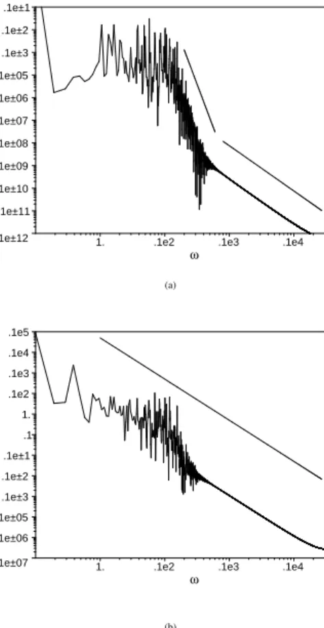
FIG. 4: Power spectra ofR(t)forA0=0.008,0.7 shown, respec-tively, in (a) and (b).
origin (kink), and therefore is a consequence of the bounded oscillatory behavior of all modal coefficients. This fact can be understood as an evidence of the stability of the kink under nonlinear perturbations.
The above results have shown that the increase of the initial perturbation induces the modal coefficients to exhibit a tran-sition from quasi-periodic to chaotic behavior. Nevertheless, another interesting feature of the overall dynamics of pertur-bations about the kink can be undertaken by the power spec-trum of the ‘radius’ defined in the space spanned by the modal coefficients,
R(t) =
Ã
N
∑
k=0 a2k
!12
,
where the originR=0 represents the kink. In Fig. 4 we depict the power spectrum ofR(t)for the linear and nonlinear per-turbations1characterized byA0=0.008 andA0=0.7, respec-tively. The first aspect worth mentioning is that in both cases the high-frequency spectrum satisfies a power lawω−k, with
k≈2, albeit the modal coefficients evolve in quite distinct
1By ‘linear’ perturbations we mean those small enough to reproduce the
regimes. This constitutes a self-similarity with respect to the strength of the perturbation. On the other hand, the effect of increasing the parameterA0is to change the power-law scal-ing present in the low-frequency domain (cf. Fig. 4(a)), for which the exponent changes fromk≈7.1 tok≈2. In this sit-uation the entire power spectrum seems to satisfy a power-law scaling as suggested by Fig. 4(b).
III. PROFILE AND STABILITY OF NIELSEN–OLESEN VORTICES
A. The static solution
In this subsection we employ the Galerkin method in order to establish the functional profile of a two-dimensional soli-ton: the Nielsen–Olesen vortex [20], which arises as a possi-ble static classical configuration for the gauge field in scalar electrodynamics (also known as the Abelian Higgs model) in the broken-symmetric phase of the scalar field. A complete analytical solution for the description of the vortex field is not available in the literature, and its profile is known through nu-merically solving the field equations of the model (in the static limit and in a particular gauge). However, the asymptotic be-havior at long distances and at the origin are known from re-quirements from finite energy and flux quantization, thus pro-viding suitable boundary conditions for the construction of a solution.
In the present case we have to deal with a coupled system of nonlinear differential equations, for which an application of the Galerkin method may contribute to obtaining a solution in a different perspective from that of pure numerical integra-tion. The method postulates an analytical form for the approx-imate solution of differential equations as a finite series on an adequate basis of functions. It remains therefore to compute the series coefficients, which is done numerically. In the case of the static Nielsen–Olesen vortex, these are obtained from solving an algebraic system of equations.
We thus consider the Abelian Higgs model, given by the following Lagrangian density for interacting scalar and vector fields:
L
=−14F
µνF
µν+¯¯Dµφ
¯ ¯ 2
−V(|φ|), (13) where Fµν(x) = ∂µAν(x) − ∂νAµ(x), Dµφ(x) =
(∂µ+ieAµ(x))φ(x) and V(|φ|) = λ
³
|φ|2−φ2 0
´2
; φ0 6= 0 is the broken-symmetry parameter andeis the electric charge of theφfield. The equations of motion are
∂µFµν+2e2|φ|2Aν = −ie(φ∗∂νφ−φ∂νφ∗), (14)
DµDµφ(x) = −2λφ
³
|φ|2−φ2 0 ´
. (15) We are interested in the evolution vortex solution with cylin-drical symmetry of the type
A(r,θ,t) = θˆA(r,t) =θˆn
er[1−F(r,t)], (16) φ(r,θ,t) = ρ(r,t)einθ, for integern. (17)
We here follow the notation of Huang’s book [21]. The cylin-drical coordinates(r,θ)are adopted in thexyplane, and one seeks a solution with cylindrical symmetry corresponding to a flux of vortex lines which is quantized in units of 2π/e. We also introduce suitable dimensionless coordinates,t→eφ0t, r→eφ0randρ→ρ/φ0, such that the field equations become
−∂
2F ∂t2 +
∂2F ∂r2 −
1 r
∂F ∂r −2ρ
2F = 0,(18)
−∂
2ρ ∂t2 +
∂2ρ ∂r2+
1 r
∂ρ ∂r−
n2F2 r2 ρ−2βρ
¡
ρ2−1¢ = 0,(19) whereβ=λ/e2. The boundary conditions are
F(0) = 1, forn6=0; lim
r→∞F(r) =0; (20)
ρ(0) = 0; lim
r→∞ρ(r) =1, (21)
and the asymptotic behaviors at the origin and infinity are (see [20, 21])
F(r)r→→01−O(r2), F(r)r→→∞const.r1/2e−√2eφ(22)0r
ρ(r)r→→0const.rn. (23)
As mentioned previously, our foremost task is to implement the Galerkin method to solve the system of differential equa-tions (18)-(19) corresponding to the static case. The idea is to recover in an efficient manner the profile of the Nielsen– Olesen vortex found only numerically, in other words provid-ing an approximate analytical expression for the fieldsF(r) andρ(r). The dynamical evolution around the static configu-ration will be subject of the next subsection. Then, we must first choose the basis of functions on which we will define the series expansion. We adopt the criterion that the basis should reflect the boundary conditions and asymptotic behav-iors above. Therefore, we introduce the rational Chebyshev functionsT Lk(x), defined in the semi-infinite interval[0,∞),
which are written in terms of ordinary Chebyshev polynomi-alsTk(x)as [22]
T Lk(x) =Tk
µ x−1 x+1
, (24)
for allk≥0. We may then define the functions ψk(r)≡(−1)k+1
1
2(T Lk+1(r)−T Lk(r)), (25) with the limiting property limr→∞ψk(r) =0, which
repro-duces the long-distance behavior ofF(r). Nevertheless, we wish that the basis also reflect the asymptotic behavior ofF(r) at the origin and this requirement leads us to use the basis functions defined by
χk(r) =
2k2+2k+1
4k+4 ψk+1(r)−
2(k+1)2+2k+3 4k+4 ψk(r),
(26) so thatχk(r)∼1−
O
(r2)near the origin. We now postulatea solutionF(r)as the finite series with real numerical coeffi-cients
F(r) =
N
∑
k=0
The constraintF(0) =1 then makes one of the coefficients, sayaN, to be expressed in terms of the remainingak’s. As
for the decomposition of theρ(r)function in some appropri-ateΦk(r)basis functions, we have itsr→∞behavior
imple-mented in the form
ρ(r) =1+
N
∑
k=0
bkΦk(r). (28)
As already mentioned, we want to choose theΦk(r)in order to
satisfy the boundary conditions, in particular near the origin, so we must require thatΦk(r)∼rn, wherenis the topological
charge. Thus we may choose a different basis for each value ofn: forn=1, we may take
Φk(r) =ψk+1(r) + 3+2k
1+2kψk(r), (29) while for n =2, Φk(r) =χk(r), and so on. In all cases,
limr→∞Φk(r) =0 and therefore ρ(r)→1 at long distances.
Also, we take the coefficientbN in (28) to be related to the
other coefficients through the conditionρ(0) =0.
If we insert both the above series decompositions of func-tions into the set of differential equafunc-tions (18), (19), and inte-grating the residuals together withχk(r)and weight function
1/r1/2(r+1)in the range[0,∞), the whole set of coefficients ak,bk may be determined, resulting in profiles forF(r)and
ρ(r) in qualitative accordance with Nielsen–Olesen [20] or Huang [21].
0 0.2 0.4 0.6 0.8 1
F
0 2 4 6 8
r
0 0.2 0.4 0.6 0.8 1
ρ
2 4 6 8
r
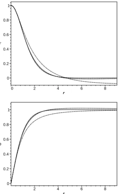
FIG. 5: Illustration of the rapid convergence of the Galerkin decom-positions forFandρgiven by Eqs. (27) and (28), respectively. We have considered truncationsN=3 (dot),N=5 (dash) andN=8 (line).
We also wish to compare our results with the de Vega– Schaposnik exactn=1 solution [23], obtained with the re-lation between coupling constantse2=2λ(in our notation). The result is that the de Vega–Schaposnik solution is accu-rately reproduced (see Figs. 1 and 2 of Ref. [23]) with just a few terms of the truncated series. In Figs. 5 (a) and (b) we see how this convergence is rapidly achieved for the solutions we have derived with the Galerkin method, with truncations N=3, 5 and 8.
B. Nonlinear stability of the vortex
We proceed now with the investigation of the general dy-namics of perturbations about the vortex configuration. For this task we use the Galerkin method to integrate the field equations (18) and (19), in which the decomposition of the fieldsF(r,t)andρ(r,t)are the same as given by Eqs. (27) and (28) but assuming time dependence of the modal coeffi-cients. The remaining steps to obtain the dynamical system are the same as already outlined previously. Thus, after a di-rect calculation we arrive at a set of equations of the form
¨
ak(t) =
F
k(aj,bj), ¨bk(t) =G
k(aj,bj), whereF
k andG
k arenonlinear functions of the modal coefficients. Basically, as we have obtained in the case of the kink, these equations con-stitute a set of nonlinear coupled oscillators.
In the abstract phase space spanned by the modal coeffi-cients(ak,bk), the static Nielsen–Olesen vortex is represented
by a fixed point P0 whose coordinates (ak(0),b(k0)) were de-termined in the last subsection. To make arbitrary pertur-bations evolve about this configuration we set initial con-ditions of the type ak(0) =a(k0)+δak(0), bk(0) =b(k0)+
δbk(0), in order to include linear and nonlinear
perturba-tions characterized by |δak(0)/a(
0)
k |,|δbk(0)/b(
0)
k | ≪1 and |δak(0)/a(k0)|,|δbk(0)/b(k0)| ∼
O
(1), respectively. Thestabil-ity of the vortex will be guaranteed if the modesδak,δbk
re-main bounded. Instead of studying the behavior of an aver-aged quantity associated to the perturbation we have consid-ered the the ‘radius’
R(t) =
"
N−1
∑
k=0
(δa2k+δb2k)
#12
.
In Fig. 6 we depict a log-linear plot ofR(t) corresponding to linear (graph at the bottom) and nonlinear (the next two graphs, for different initial strengths) perturbations about the Nielsen–Olesen vortex corresponding toβ=0.5,n=1. No-tice thatR(t)has a bounded oscillatory behavior which consti-tutes a good numerical evidence of the stability of the vortex beyond the linear perturbation scheme.
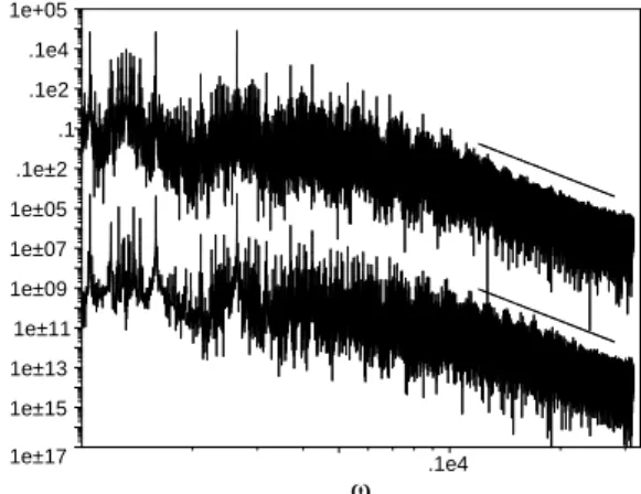
self-similarity with respect to the initial strength of the per-turbation. In particular note that domain of high frequencies satisfies a power-law scaling,ω−k, withk≈7.16.
1e–05 .1e–3 .1e–2 .1e–1 .1 1. .1e2
R
5 10 15 20 25
t
FIG. 6: Log-linear plot of the ‘radius’ versus time for linear and nonlinear perturbations (from the bottom to the top) about the vor-tex configuration. We have considered the caseβ=0.5,n=1 and truncationN=8.
1e–17 1e–15 1e–13 1e–11 1e–09 1e–07 1e–05 .1e–2 .1 .1e2 .1e4 1e+05
.1e4
ω
FIG. 7: Log-log plot of the power spectrum ofR(t) in the linear and nonlinear regime of the modal coefficients. The domain of high frequencies is well fitted with the power-law scalingω−kwherek≈
7.16. On the other hand, the effect of increasing the initial strength of perturbations reflects in the low-frequency range of the spectrum, where the peaks are split in a large number of components.
IV. CONCLUSIONS
In this paper we have studied the evolution of linear and nonlinear perturbations of the topological kink configuration of scalar field theories with quartic potential in the broken-symmetric phase, and of the Nielsen–Olesen vortex in scalar electrodynamics. We have applied the Galerkin method with two objectives in mind: (i) to reconstruct the Nielsen–Olesen vortex with a relatively low truncation order due to the appro-priate choice of the trial functionsχk(r)andΦk(r)(cf. Eqs.
(26) and (29)); (ii) to tackle the nonlinear partial differential equations that govern the dynamics of arbitrary perturbations about the kink and the vortex static configurations. These equations were then approximated to dynamical systems in an abstract phase space according to the Galerkin method. In this phase space the solitonic configurations are represented by well-defined fixed points, and linear stability is guaranteed by the stable nature of these fixed points under small depar-tures.
The numerical experiments have indicated that both soli-tonic configurations are indeed stable under nonlinear pertur-bations. In both cases very small perturbations may be in-terpreted as the motion of an orbit on a torus embedded in the phase space of the modal coefficients. The increase of the initial perturbation produces the transition from regular to chaotic by the breaking of the KAM torus (as suggested in Fig. 3), and possibly exhibiting Arnold diffusion which is typical in Hamiltonian systems with more than two degrees of freedom. The relevant consequence of this nontrivial dy-namics emerges after constructing the power spectrum of the distanceR(t)from the fixed point representing the kink or the vortex. Then, from Figs. 4 and 7 we have shown that the power spectra satisfy a power lawω−k valid within a large
range of frequencies, wherekassumes distinct values depend-ing whether the kink or vortex perturbations are considered. The increase of the strength of initial perturbations seems not to alter the power law. There is thus the implication of self-similarity with respect to this increase. Therefore, the dynam-ics of perturbations about the solitonic configuration as de-scribed byR(t)reveals to be complex, even though the modal coefficients evolve in the linear regime.
As our closing remarks, we believe that our approach has opened an fertile venue for treating the dynamics of nonlinear perturbations about the solitonic configurations under consid-eration. Physically, such nonlinear perturbations can be of interest in condensed-matter systems as well as in cosmology. As a next step, we intend to extend our analysis to the case of the ’t Hooft–Polyakov monopole [24]. In this instance, it will be important to verify whether the self-similarity is also present in this other situation, along with trying to provide a clearer physical implication of such self-similarity. Finally, we must point out several works that were devoted to the study of chaos in gauge theories with vortices and monopoles so-lutions [25], in which the authors have used a different ap-proximative scheme and have focused in the evaluation of the Lyapunov exponents associated to the soliton energy to char-acterize chaos.
APPENDIX A
χkandΦk, respectively (cf. Eqs. (25 and (28)). We have
con-sidered the truncation orderN=8, and after performing the Galerkin procedure a set of algebraic equations for the modal
coefficientsak andbk is obtained. For the sake of
complete-ness we exhibit the expressions ofF(r)andρ(r) correspond-ing to the caseβ=1/2 parameter:
F(r) = 0.840376 2r+1
(r+1)2−0.221538
8r2−3r−1
(r+1)3 −0.0173983
54r3−145r2+12r+3
(r+1)4 +0.0214648× (A1) 32r4−203r3+161r2−5r−1
(r+1)5 +0.0026529
5+30r−2010r2+5376r3−2835r4+250r5
(r+1)6 (A2)
−0.000161889−21r+2530r
2−11682r3+12969r4−3817r5+216r6−3
(r+1)7 −0.0004730614285714286×(A3)
7+56r−11011r2+78078r3−148863r4+686r7−17381r6+92092r5
(r+1)8 − (A4)
0.00161165−1−9r+2695r
2−27209r3+79365r4+128r8−4395r7+33397r6−84227r5
(r+1)9 (A5)
−0.00003385411
(r+1)10 (9+90r−38964r
2+531216r3−2199834r4+1458r9−65127r8+670752r7 (A6)
−2426580r6+3568708r5) (A7)
ρ(r) = 1−1.1057(r+1)−2+0.00809072 5r−1
(r+1)3+0.05115296
35r2−42r+3
(r+1)4 +0.01837782857142857× (A8)
,21r
3−63r2+27r−1
(r+1)5 −0.008523333
5−220r+990r2−924r3+165r4
(r+1)6 −0.009276436363636364× (A9) 195r−1430r2+2574r3−1287r4+143r5−3
(r+1)7 −
0.0009448492307692308
(r+1)8 (7−630r+6825r
2−20020r3(A10)
+19305r4+455r6−6006r5) +0.000175872
(r+1)9 (119r−1785r 2+
7735r3−12155r4+85r7−1547r6+7293(A11)r5
−1) +0.00003187141806342447
(r+1)10 (−1368r+27132r 2
−162792r3+377910r4+969r8−23256r7+ (A12)
151164r6−369512r5+9). (A13)
By choosing other values of β the solution of the algebraic equations can be determined directly.
AcknowledgmentsH. P. O. acknowledges CNPq/Brazil for partial financial support. Figs. 2 were generated using the
Dy-namics Solverpackage [19].
[1] A. C. Scott, F. Y. F. Chu, and D. W. McLaughlin, Proc. IEEE 61, 1443 (1973).
[2] R. Rajaraman, Phys. Rep.21, 227 (1975);ibid., Solitons and
Instantons, North-Holland, Amsterdam, 1989.
England, 1994.
[4] D. W. MacLaughlin and A. C. Scott, Phys. Rev. A18, 1652 (1978).
[5] T. I. Belova and A. E. Kudryavtsev, Physics-Uspekhi40, 359 (1997).
[6] M. B. Fogel, S. E. Trullinger, A. R. Bishop, and J. A. Krumhansl, Phys. Rev. B15, 1578 (1977).
[7] J. Rubinstein, J. Math. Phys.11, 258 (1970).
[8] N. R. Quintero and A. Sanchez, Eur. Phys. J. B6, 133 (1998). [9] V. G. Makhankov, Phys. Rep.35, 1 (1978).
[10] C. A. J. Fletcher,Computational Galerkin Methods, Springer-Verlag, New York, 1984.
[11] D. Gottlieb and S. A. Orszag,Numerical Analysis of Spectral Methods: Theory and Applications, SIAM, Philadelphia, 1977. [12] P. Holmes, J. L. Lumley, and G. Berkooz,Turbulence, Coher-ent Structures, Dynamical Systems and Symmetry, Cambridge University Press, Cambridge, UK, 1996.
[13] C. N. Kumar and A. Khare, J. Phys. A: Math. Gen.22, L849 (1989); B. Dey, C. N. Kumar and A. Sen, Int. J. Mod. Phys. A 8, 1755 (1993).
[14] T. S. Bir´o, S. G. Matynian, and B. M¨uller,Chaos and Gauge Field Theory, World Scientific, Singapore, 1994.
[15] V. L. Ginzburg and L. D. Landau, Zh. Eksp. Teor. Fiz.20, 1064
(1950); L. P. Gorkov, Zh. Eksp. Teor. Fiz.36, 1364 (1959). [16] M. Goodband and M. Hindmarsh, Phys. Rev. D 52, 4621
(1995).
[17] W. H. Press, S. A. Teukolsky, W. T. Wetterling, and B. P. Flan-nery, Numerical Recipes in C: The Art of Scientific Comput-ing, 2nd edition, Cambridge University Press, Cambridge, UK, 1992.
[18] A. R. Bishop, K. Fesser, and P. S. Lomdahl, Physica D7, 259 (1983).
[19] J. M. Aguirregabiria, Dynamics Solver, http://tp.lc.ehu.es/jma.html.
[20] H. B. Nielsen and P. Olesen, Nucl. Phys. B61, 45 (1973). [21] K. Huang,Quarks, Leptons & Gauge Fields, World Scientific,
Singapore, 1982.
[22] J. P. Boyd,Chebyshev and Fourier Spectral Methods, Dover, New York, 2001.
[23] H. J. de Vega and F. Schaposnik, Phys. Rev. D14, 1100 (1976). [24] G. ’t Hooft, Nucl. Phys. B79, 276 (1974); A. M. Polyakov,
JETP Lett.20, 194 (1974),.