ACPD
8, 18385–18407, 2008Relating observations of contrail persistence
to numerical
D. P. Duda et al.
Title Page
Abstract Introduction
Conclusions References
Tables Figures
◭ ◮
◭ ◮
Back Close
Full Screen / Esc
Printer-friendly Version
Interactive Discussion
Atmos. Chem. Phys. Discuss., 8, 18385–18407, 2008 www.atmos-chem-phys-discuss.net/8/18385/2008/ © Author(s) 2008. This work is distributed under the Creative Commons Attribution 3.0 License.
Atmospheric Chemistry and Physics Discussions
This discussion paper is/has been under review for the journalAtmospheric Chemistry and Physics (ACP). Please refer to the corresponding final paper inACPif available.
Relating observations of contrail
persistence to numerical weather analysis
output
D. P. Duda1, R. Palikonda2, and P. Minnis3
1
National Institute of Aerospace, Hampton, VA, USA
2
Science Systems and Applications, Inc., Hampton, VA, USA
3
Science Directorate, NASA Langley Research Center, Hampton, VA, USA
Received: 7 April 2008 – Accepted: 2 October 2008 – Published: 21 October 2008 Correspondence to: D. P. Duda ([email protected])
ACPD
8, 18385–18407, 2008Relating observations of contrail persistence
to numerical
D. P. Duda et al.
Title Page
Abstract Introduction
Conclusions References
Tables Figures
◭ ◮
◭ ◮
Back Close
Full Screen / Esc
Printer-friendly Version
Interactive Discussion
Abstract
The potential for using high-resolution meteorological data from two operational numer-ical weather analyses (NWA) to diagnose and predict persistent contrail formation is evaluated using two independent contrail observation databases. Contrail occurrence statistics derived from surface and satellite observations between April 2004 and June
5
2005 are matched to the humidity, vertical velocity, wind shear and atmospheric sta-bility derived from analyses from the Rapid Update Cycle (RUC) and the Advanced Regional Prediction System (ARPS) models. The relationships between contrail oc-currence and the NWA-derived statistics are analyzed to determine under which at-mospheric conditions persistent contrail formation is favored within NWAs. Humidity is
10
the most important factor determining whether contrails are short-lived or persistent, and persistent contrails are more likely to appear when vertical velocities are positive, and more likely to spread when the atmosphere is less stable. Although artificial up-per limits on upup-per tropospheric humidity within the NWAs prevent a direct quantitative agreement of model data with contrail formation theory, logistic regression or similar
15
statistical methods may improve the prediction of contrail occurrence.
1 Introduction
Contrail-induced cloud cover has the potential to produce significant regional effects on climate (Minnis et al., 2004). As air traffic increases, the possibility for globally sig-nificant impacts also rises. Although these impacts, such as radiative forcing, have
20
been estimated using general circulation models (GCMs) (Marquart and Mayer, 2002; Hansen et al., 2005), their magnitudes remain highly uncertain because of the rela-tively crude ways that contrails are parameterized in those models. One approach to improve contrail representations and to understand and predict contrail climate effects better, is to develop models that can more accurately simulate contrail properties at
25
ACPD
8, 18385–18407, 2008Relating observations of contrail persistence
to numerical
D. P. Duda et al.
Title Page
Abstract Introduction
Conclusions References
Tables Figures
◭ ◮
◭ ◮
Back Close
Full Screen / Esc
Printer-friendly Version
Interactive Discussion
humidity, and winds and then parameterize those models for inclusion in GCMs. Higher resolution contrail models could also be useful for aiding contrail mitigation efforts, if that need arises. To perform such simulations, it is critical to have meteorological data at high temporal and spatial resolutions over a large domain because air traffic over a given location changes rapidly throughout the day. Only a few operational
numer-5
ical weather analyses (NWA), including the NOAA/ESRL Rapid Update Cycle (RUC; Benjamin et al., 2004) and the Advanced Regional Prediction System (ARPS; Xue et al., 2003) produced by the University of Oklahoma Center for Analysis and Prediction of Storms, currently provide those variables at the resolutions necessary to diagnose persistent contrail formation over the United States of America.
10
The basic thermodynamics of contrail formation from jet exhaust was described by Schmidt/Appleman theory (Schumann, 1996), which has been modified more recently to account for the effects of jet aircraft efficiency. This theory describes the tempera-ture and pressure conditions necessary to allow the isobaric mixing of the hot, moist exhaust gases with the cold ambient air to form a contrail. The formation of persistent
15
contrails occurs when the relative humidity with respect to ice (RHI) reaches or ex-ceeds 100%. A review of the historical development of the theory and its experimental verification is given in Schumann (1996). NWAs, however, often underestimate upper tropospheric relative humidity (UTH) due to large dry biases in the balloon soundings used to construct the analyses and to internal adjustments made to meet the model’s
20
physical constraints (Minnis et al., 2005b). Although this dry bias prevents a straightfor-ward determination of persistent contrail formation via Schmidt/Appleman theory, such a dry bias might be correctable if the numerical weather humidity data can be shown to be consistent with the appearance or non-appearance of contrails. Thus, one out-standing problem that must be addressed before a realistic simulation of contrails can
25
be achieved is to determine how accurately the meteorological data provided by the numerical weather analyses and forecasts diagnose contrail formation conditions.
ACPD
8, 18385–18407, 2008Relating observations of contrail persistence
to numerical
D. P. Duda et al.
Title Page
Abstract Introduction
Conclusions References
Tables Figures
◭ ◮
◭ ◮
Back Close
Full Screen / Esc
Printer-friendly Version
Interactive Discussion
To achieve that goal, we match several months of contrail occurrence statistics derived from satellite and surface observations to the NWA-derived humidity, vertical velocity, wind shear and atmospheric stability. The relationships between contrail occurrence and the NWA-derived statistics are then analyzed to determine under which atmo-spheric conditions the formation of persistent contrails is favored.
5
2 Data and methodology
Two independent types of contrail observations are used to evaluate the NWA models. Satellite data can reveal contrails above lower level clouds that are missed by surface observers, but are biased, on average, toward lower occurrence rates. Surface ob-servers can provide more reliable contrail observations and detect some of the thinner
10
contrails missed by the satellite.
2.1 Surface data
The Global Learning and Observations to Benefit the Environment (GLOBE) program collects observations of cloud occurrence and coverage throughout the contiguous United States (CONUS) from primary and secondary schools across the country. (See
15
www.globe.gov for more information about the GLOBE program.) In May 2003, GLOBE initiated a contrail observation protocol to measure and classify contrail observations. A primary goal of the GLOBE program is to use detailed written protocols to enable students to provide scientifically valuable measurements of environmental parameters (Brooks and Mims, 2001). Over 18 500 observations were reported over the region
20
between 1 April 2004 and 27 June 2005. The observations usually include contrail cov-erage, contrail number, cloud covcov-erage, cloud type and a classification of contrails into three categories, short-lived (SHRT), non-spreading persistent contrails (NSPR), and spreading persistent contrails (SPRD). The contrail categories are defined as follows: short-lived contrails are contrails that dissipate as the aircraft moves across the sky.
ACPD
8, 18385–18407, 2008Relating observations of contrail persistence
to numerical
D. P. Duda et al.
Title Page
Abstract Introduction
Conclusions References
Tables Figures
◭ ◮
◭ ◮
Back Close
Full Screen / Esc
Printer-friendly Version
Interactive Discussion
Persistent contrails are contrails that remain in the sky after the aircraft has flown out of view of the observer. Spreading contrails are defined as persistent contrails wider than the width of a finger held at arm’s length. This width corresponds to a contrail that is 2◦s of arc wide, or at least 350 m wide (based on a contrail altitude of 10 km) (O’Shea,
1991), which is the minimum width expected to be detectable in NOAA’s Advanced Very
5
High Resolution Radiometer (AVHRR) imagery. The cloud coverage observations are reported within six categories based on total coverage of non-contrail cloudiness: no clouds (0% coverage), clear (1–9% coverage), isolated (10–24% coverage), scattered (25–49% coverage), broken (50–89% coverage) and overcast (90–100% coverage).
The GLOBE contrail dataset contains observations from 417 schools. The schools
10
are mostly located in highly populated regions with substantial air traffic (Fig. 1). Only 123 of the schools (29.5%) reported more than 30 observations during the 15-month time period, but those schools reported 16 008 observations, 86.5% of the total. Nearly all schools reported only one observation/day. Approximately 92% of all observations were between 14:30 and 20:30 UTC, and nearly 58% of the total were between 16:30
15
and 18:30 UTC.
To test the quality of the surface-based observations, the set of 11 schools that had at least 50 observations taken under mostly clear skies (non-contrail cloud coverage less than 25%) were chosen for closer study. Because these schools provided multi-ple observations throughout the period, we expect that these locations would be more
20
likely to provide high quality contrail observations among the GLOBE participants than locations with few contrail reports. Figure 1 shows the location of the 11 schools as a large black plus (+) sign. All schools with the exception of Box Elder, Montana are located in regions with substantial commercial air traffic during the typical observa-tion period. From these schools, a uniformly random sample of 379 GLOBE contrail
25
ob-ACPD
8, 18385–18407, 2008Relating observations of contrail persistence
to numerical
D. P. Duda et al.
Title Page
Abstract Introduction
Conclusions References
Tables Figures
◭ ◮
◭ ◮
Back Close
Full Screen / Esc
Printer-friendly Version
Interactive Discussion
servations are sorted into four categories. Category A indicates that both the surface and satellite observations detected contrails, while category D shows the cases where both methods detected no contrails. Category B includes the occasions when contrail occurrence was detected by satellite but not reported by the student observers, and category C include the observations when the surface observer reported persistent
5
contrails while none were apparent in the satellite imagery. The surface and satellite observations matched nearly 75% of the time (categories A and D), while 18% of the observations were in category C, and the remaining 7% of observations were in cate-gory B. As a test of the integrity of the surface and satellite observations, the maximum relative humidity with respect to ice (RHI) within the upper troposphere (between 150
10
and 400 hPa) was determined from the ARPS analyses for each observation, and the mean for each observation category is presented in Table 1. The mean ARPS RHI for category A observations was 88.2%, while the mean ARPS RHI was only 48.3% when both observations showed no contrails (category D). It is important to note some dif-ferences between surface-based and satellite-based observations. Surface observers
15
often miss contrails forming above lower cloudiness (although by choosing only mostly clear observations, this type of error should be minimal here), misidentify linear cloud features as contrails (or contrails as cloud streaks), or record the observation incor-rectly in the contrail report. Cloud cover and the misidentification of cloud streets as contrails also hamper the visual detection of persistent contrails in the GOES satellite
20
imagery loops. Surface observers, however, can detect much narrower and probably optically thinner contrails than those seen in the 4-km resolution GOES satellite im-agery. Some of the cases where observers reported contrail coverage not seen in the satellite (category C) may have been due to the observation of non-spreading persis-tent contrails that could not be detected in the GOES imagery loops. In addition, over
25
ACPD
8, 18385–18407, 2008Relating observations of contrail persistence
to numerical
D. P. Duda et al.
Title Page
Abstract Introduction
Conclusions References
Tables Figures
◭ ◮
◭ ◮
Back Close
Full Screen / Esc
Printer-friendly Version
Interactive Discussion
between categories C and D at the three schools supports the possibility of this type of error.
2.2 Satellite data
Multi-spectral data from the AVHRR onboard the NOAA-16 satellite were used to iden-tify linear contrails (Lee, 1989) following the contrail detection algorithm of Mannstein et
5
al. (1999) as applied by Palikonda et al. (2005). The Mannstein et al. (1999) algorithm uses a combination of channel 4 (10.8-µm) and channel 5 (12.0-µm) radiances to iden-tify contrails. Radiance data were collected from 366 mid-afternoon overpasses of the satellite between April 16, 2004 and June 27, 2005 within a 4×6◦grid box over eastern
Ohio/western Pennsylvania/West Virginia (38◦–42◦N; 78◦–84◦W), an area selected be-10
cause of its heavy commercial air traffic (Garber et al., 2005). During the observation period, contrails were detected within 43.3% of all available grid boxes, while cirrus was detected within 47.7% of the available grid boxes. Minnis et al. (2005a) and Pa-likonda et al. (2005) found that the technique tends to overestimate contrail coverage by 20–40% mainly because of natural cirrus that appears much like contrails.
15
2.3 Meteorological data
Meteorological data from the high-resolution, hourly RUC-20 analyses and ARPS anal-yses and forecasts provide information on temperature, humidity, pressure, and vertical velocity that is matched with each of the surface and satellite observations. The RUC-20 data have a resolution of RUC-20 km, while the ARPS data were obtained from the 27-km
20
resolution, hourly CONUS domain analyses. The ARPS forecasts are 1-day (16–20 h), 2-day (40–44 h), and 3-day (64–68 h) forecasts from 16:00 UTC to 20:00 UTC.
To match the surface and meteorological data, data from the RUC analyses closest in time with the contrail observations are bilinearly interpolated to the location of each observation. An observation is not used if the time difference between the observation
25
ACPD
8, 18385–18407, 2008Relating observations of contrail persistence
to numerical
D. P. Duda et al.
Title Page
Abstract Introduction
Conclusions References
Tables Figures
◭ ◮
◭ ◮
Back Close
Full Screen / Esc
Printer-friendly Version
Interactive Discussion
the maximum relative humidity with respect to ice (RHImax) is determined from all levels (spaced at every 25 hPa) that have a temperature less than or equal to −40◦C. The
temperature constraint was added to eliminate areas where the atmosphere is likely to be too warm to form contrails (Appleman, 1953). Although the observed contrails may have formed at other levels, this level was chosen as the most likely level for contrail
5
formation, and to provide a consistent representation of humidity at typical commercial aircraft flight levels. The probability distribution function of the level of RHImaxis roughly Gaussian in shape for both the RUC and ARPS analyses with a maximum around 250 hPa.
All other meteorological data (including vertical velocity) are selected from this level
10
for comparison with the surface observations of contrail occurrence. The vertical shear of the horizontal wind and the temperature lapse rate for the 25-hPa layer below the level of maximum RHI are also computed. The vertical velocity, the lapse rate (a mea-sure of the atmospheric stability) and the vertical shear are expected to influence the spreading rate of persistent contrails (Jensen et al., 1998).
15
A similar procedure is used to match the ARPS upper tropospheric data with the surface-based contrail observations. The RHI is computed from the ARPS fields of potential temperature and specific humidity at the 25-hPa intervals to determine the level of maximum upper tropospheric humidity.
To compare NWA output with the satellite observations, contrail and cirrus
occur-20
rence statistics are derived for each 1×1◦grid box within the 4×6◦observation domain.
Contrail occurrence is determined for each grid box from the automated linear con-trail detection algorithm while cirrus occurrence is determined by visual inspection of infrared imagery from each satellite overpass. Meteorological data (including RHI, ver-tical velocity, wind shear and atmospheric lapse rate) from the RUC and ARPS are then
25
linearly interpolated to the center of each 1×1◦ box within the domain to correlate the
ACPD
8, 18385–18407, 2008Relating observations of contrail persistence
to numerical
D. P. Duda et al.
Title Page
Abstract Introduction
Conclusions References
Tables Figures
◭ ◮
◭ ◮
Back Close
Full Screen / Esc
Printer-friendly Version
Interactive Discussion
period.
3 Results
3.1 Comparison of NWA output with surface observations
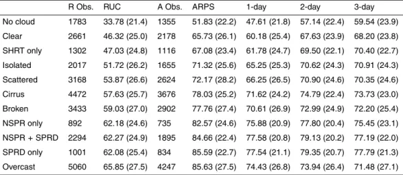
Contrail coverage was reported in 27.0% of a total of 18 504 surface observations. At least one persistent (either spreading or non-spreading) contrail was reported in 17.0%
5
of the observations. This frequency is slightly higher than Minnis et al. (1993) for the highest period of contrail occurrence, 1993–1994: 15.2% for unobscured skies. Most of the GLOBE data (80.1%) were taken during the non-summer months when contrail coverage is greater. Similar to the US Air Force observers in the Minnis et al. study, the highest contrail frequencies were reported from October through April (18.8%), while
10
the lowest contrail frequencies were reported from June through September (12.0%). Most of the persistent contrail observations (71.3%) were made in partly cloudy skies (either clear skies, or skies with isolated or scattered cloudiness). Table 2 shows the mean value of RHImax calculated from the collocated RUC and ARPS analyses for several cloudiness categories.
15
The increase in RHImax with increasing cloud coverage category suggests that the GLOBE cloud and contrail observations were consistent with the numerical weather output, as the largest RHImaxvalues occurred when overcast skies were reported. Al-though most persistent contrails were observed under partly cloudy conditions, the RHIs computed by both numerical weather analyses were higher when persistent
con-20
trails formed than under usual partly cloudy conditions. Table 2 shows that persistent contrails form as expected in high humidity environments, although a comparison be-tween the mean RHImaxfor persistent contrails (the category NSPR+SPRD) with the minimum RHI required by the Schmidt/Appleman criteria (100%) demonstrates that both models show a dry bias of at least 15 to 38% when compared to contrail
for-25
ACPD
8, 18385–18407, 2008Relating observations of contrail persistence
to numerical
D. P. Duda et al.
Title Page
Abstract Introduction
Conclusions References
Tables Figures
◭ ◮
◭ ◮
Back Close
Full Screen / Esc
Printer-friendly Version
Interactive Discussion
occurred when persistent spreading contrails were present. The dry bias is expected as both models limit upper tropospheric moisture. Even though ice supersaturation is common in the upper troposphere and has been measured to be as high as 150% (e.g., Miloshevich et al., 2001), the RUC-20 analyses do not allow ice supersaturation to exceed 100% by more than a few percent at pressures below 300 hPa. The
RUC-5
20 mean value of RHI for overcast clouds is∼15% less than that found by Minnis et
al. (2005b) when comparing RUC-2 RHI with clouds having temperatures below−40◦C.
This difference reflects the change in upper tropospheric humidity processing scheme between RUC-2 and RUC-20 to limit RHI artificially in the RUC-20. The ARPS analy-ses allow some ice supersaturation, although RHI values rarely exceed 112%. No ice
10
supersaturation occurs in the ARPS forecasts; the maximum RHI is only 100 percent. This difference between the analyses and forecasts could account for the marked drop in the RHI values in the forecasts shown in Table 2.
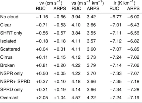
Table 3 shows the mean values of vertical velocity (vv), vertical wind shear (vs), and atmospheric lapse rate (lr) from the RUC and ARPS collocated with the surface contrail
15
observations from GLOBE. Although most persistent contrails were reported under partly cloudy conditions, the RUC and ARPS vertical velocities were larger than the mean vertical velocities reported under such cloudiness conditions. When persistent contrails were present, the vertical shear of the horizontal wind was similar to the shear analyzed under typical partly cloudy conditions. The temperature lapse rate at the
20
level of maximum RHI indicates the stability of the atmosphere where contrails form, and helps determine the depth of persistent contrails. Contrails will tend to be thicker vertically as the magnitude of the lapse rate increases (i.e., the atmosphere becomes less stable). Table 3 shows that the largest mean lapse rates occur in both the RUC and ARPS analyses when spreading persistent contrails are reported.
25
3.2 Comparison of NWA output with satellite observations
ACPD
8, 18385–18407, 2008Relating observations of contrail persistence
to numerical
D. P. Duda et al.
Title Page
Abstract Introduction
Conclusions References
Tables Figures
◭ ◮
◭ ◮
Back Close
Full Screen / Esc
Printer-friendly Version
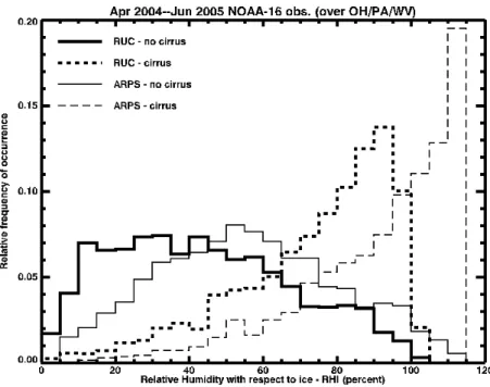
Interactive Discussion
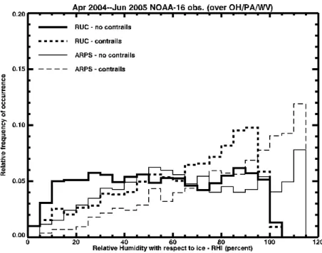
and ARPS models are separated into grid boxes containing contrails (dashed lines) and boxes with no contrails (solid lines). The contrail distributions are skewed toward higher RHI values, but the “no contrail” distributions are relatively uniform. The distribu-tions in Fig. 2b, which are separated by the presence or absence of cirrus, show a clear distinction in the humidity between the cirrus and non-cirrus grid boxes. Figure 2b
sug-5
gests that the NWAs may be better at predicting cirrus than contrail occurrence. The demarcation seen in Fig. 2b suggests that for the ARPS analyses, a simple threshold near 75% RHI would accurately predict cirrus occurrences while for the RUC analyses the best threshold would be between 60 and 65%.
To assess the skill level of such an RHI-based forecast, three measures of
fore-10
casting skill were computed. The skill scores were constructed using a simple 2-by-2 forecast matrix with the following outcomes:ais the number of cases where the RHI is at or above the threshold and cloud is observed in the grid box (hits);bis the number of cases where RHI is at or above the threshold but no cloud is observed (false alarms); cis the number of cases where RHI is below the threshold but a cloud is observed
15
(misses); anddis the number of cases where RHI is below the threshold and no cloud is observed (correct rejections). The three skill measures are:
Hit rate. The hit rate is (a+d)/(a+b+c+d), and represents the percentage of fore-casts in which the method correctly predicted the observed event.
Bias ratio. The bias ratio is computed from (a+b)/(a+c), and measures the tendency
20
of a forecast method to over- or under-forecast the occurrence of contrails or cirrus. A perfectly unbiased method would have a bias ratio of 1.00, while values below unity indicate that the cirrus/contrail occurrence is under-forecasted, and values above unity indicate that cirrus/contrail occurrence is over-forecasted.
Heidke Skill Score (HSS). The HSS is calculated as HSS=2(ad–bc)/(a+c)(c+d)–
25
ACPD
8, 18385–18407, 2008Relating observations of contrail persistence
to numerical
D. P. Duda et al.
Title Page
Abstract Introduction
Conclusions References
Tables Figures
◭ ◮
◭ ◮
Back Close
Full Screen / Esc
Printer-friendly Version
Interactive Discussion
random forecasts.
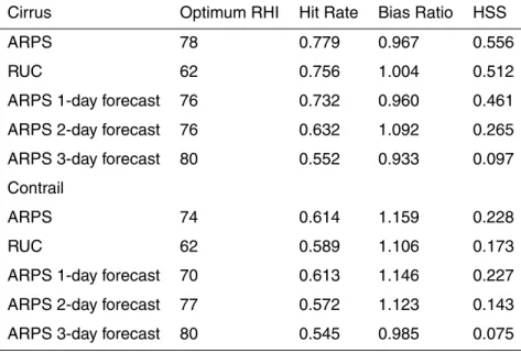
Table 4 shows the hit rate, bias ratio and HSS computed for the best-case RHI threshold chosen for each NWP analysis/forecast for both cirrus and contrail occur-rence. The optimal RHI for each case was determined by finding the particular RHI threshold that maximizes HSS. The HSS-optimized thresholds also tended to have the
5
highest hit rates, and the bias ratios usually were close to 1.00. As expected, the cir-rus occurrence forecasts were much better than the contrail occurrence forecasts for both analyses. Because cirrus and contrails can only form in supersaturated regions, the optimal RHI should be at least 100%. Thus, both the RUC and the ARPS have a dry bias. Some dry bias is expected because the model analyses produce a grid
10
average relative humidity such that the model would only register 100% if the entire grid box were covered in clouds. The difference in the skill scores between the RUC and ARPS analyses is not as large as the difference in the cirrus skill scores compared to the contrail skill scores. The higher cirrus skill scores confirm that the model analy-ses do much better representing moisture where cirrus appears than where persistent
15
contrails appear.
4 Discussion and conclusions
The results in Table 2 confirm that relative humidity is the most important factor deter-mining whether contrails are short-lived or persistent. Although most surface observa-tions of contrails occur in clear or partly cloudy skies, the UTH observed when
persis-20
tent contrails form is typically much higher than the average humidities observed under partly cloudy conditions, or when only short-lived contrails are reported. The RHI val-ues reported when spreading persistent contrails are observed are slightly larger than when non-spreading persistent contrails are reported (at least in the ARPS analyses), suggesting that humidity is one factor influencing the formation of spreading contrails.
25
ACPD
8, 18385–18407, 2008Relating observations of contrail persistence
to numerical
D. P. Duda et al.
Title Page
Abstract Introduction
Conclusions References
Tables Figures
◭ ◮
◭ ◮
Back Close
Full Screen / Esc
Printer-friendly Version
Interactive Discussion
appear when the vertical velocities are positive than when negative, and the contrails may be more likely to spread when the atmosphere becomes less stable. Although vertical shear is the primary mechanism responsible for spreading contrails, the mag-nitude of the shear appears to be less important in determining whether contrails will spread than the other factors. It is likely that sufficient UTH and atmospheric instability
5
is necessary to make contrails deep enough and long-lived so that the wind shear can spread the clouds. Another result of this study is that simple humidity thresholds in the numerical weather analyses may be appropriate for determining where cirrus is likely to form. The prognosis of contrails from relative humidity analyses is complicated by the occasional lack of contrail formation when UTH is high. This may be the result of cirrus
10
clouds competing with contrails for atmospheric moisture and obscuring the detection of any contrails that formed. It might also be due to errors in the UTH diagnosed by the models, or simply to the lack of jet air traffic in the region. Other factors that can affect the determination of contrails or cirrus from NWAs are input data such as satellite radi-ances or cloud-top heights. Inclusion of those parameters into the numerical weather
15
analyses can, in many instances, force the model to increase or decrease the UTH to match the observations resulting in the relatively good diagnoses of cirrus-related pa-rameters seen here. However, such data are available only in an analysis model and would only contribute to the diagnoses in a forecast model indirectly by improving the forecast. A comparison of the forecast skill statistics in Table 4 shows that the simple
20
RHI threshold model loses much forecast skill in predicting cirrus occurrence after 24 h. Because the intent of this paper is to demonstrate the overall applicability of NWA data to predict contrail occurrence, no consideration is given here to the spatial or seasonal variations in these atmospheric variables. More insight may be gained in future studies by looking at spatial or seasonal differences in the contrail occurrence
25
data.
ACPD
8, 18385–18407, 2008Relating observations of contrail persistence
to numerical
D. P. Duda et al.
Title Page
Abstract Introduction
Conclusions References
Tables Figures
◭ ◮
◭ ◮
Back Close
Full Screen / Esc
Printer-friendly Version
Interactive Discussion
placed on UTH in both analyses. This arbitrary cutoff of supersaturation removes information about the humidity field that prevents a straightforward application of Schmidt/Appleman theory, which requires accurate temperature and relative humidity data. The results of Table 4 demonstrate that forecast models based on RUC/ARPS hu-midity alone have limited skill in diagnosing contrail occurrence. Despite these results,
5
the humidity data do show some consistency with persistent contrail occurrence, and it is likely that contrail forecasts could be improved by using logistic regression (Jackson et al., 2001; Travis et al., 1997) or other statistical methods that can include several meteorological parameters in the prognosis. We plan such a multi-variable analysis in an ongoing study. However, because upper tropospheric humidity is the main factor
10
determining contrail formation, contrail forecasts will remain somewhat limited in ac-curacy until accurate assimilation of ice supersaturation is incorporated into numerical weather analyses and models. It is encouraging that the latest versions of both the RUC and the ARPS at the time of this writing are now producing significantly greater levels of ice supersaturation than were available for comparisons with the observations
15
used in this study.
Acknowledgements. This material is based upon work supported by the NASA Earth Science Enterprise Radiation Sciences Division, NASA contracts NAG1-02044 and NCCI-02043 NIA-2579, and by the National Science Foundation under Grant No. 0222623.
References
20
Appleman, H.: The formation of exhaust condensation trails by jet aircraft, B. Am. Meteor. Soc., 34, 14–20, 1953.
Benjamin, S. G., D ´ev ´enyi, D., Weygandt, S. S., Brundage, K. J., Brown, J. M., Grell, G. A., Kim, D., Schwartz, B. E., Smirnova, T. G., Smith, T. L., and Manikin, G. S.: An hourly assimilation– forecast cycle: The RUC, Mon. Weather Rev., 132, 495–518, 2004.
25
ACPD
8, 18385–18407, 2008Relating observations of contrail persistence
to numerical
D. P. Duda et al.
Title Page
Abstract Introduction
Conclusions References
Tables Figures
◭ ◮
◭ ◮
Back Close
Full Screen / Esc
Printer-friendly Version
Interactive Discussion
Garber, D., Minnis, P., and Costulis, P. K.: A commercial flight track database for upper tro-pospheric aircraft emission studies over the USA and southern Canada, Meteorol. Z., 14, 445–452, 2005.
Hansen, J., Sato, M., Ruedy, R., Nazarenko, L., Lacis, A., Schmidt, G. A., Russell, G., Aleinov, I., Bauer, M., Bauer, S., Bell, N., Cairns, B., Canuto, V., Chandler, M., Cheng, Y., Del Genio,
5
A., Faluvegi, G., Fleming, G., Friend, A., Hall, T., Jackman, C., Kelley, M., Kiang, N., Koch, D., Lean, J., Lerner, J., Lo. K., Menon, S., Miller, R., Minnis, P., Novakov, T., Oinas, V., Perlwitz, Ja., Perlwitz, Ju., Rind, D., Romanou, A., Shindell, D., Stone, P., Sun, S., Tausnev, N., Thresher, D., Wielicki, B., Wong, T., Yao, M., and Zhang, S.: Efficacy of climate forcings, J. Geophys. Res., 110, D18104, doi:10.1029/2005JD005776, 2005.
10
Jackson, A., Newton, B., Hahn, D., and Bussey, A.: Statistical contrail forecasting, J. Appl. Meteorol., 40, 269–279, 2001.
Jensen, E. J., Ackerman, A. S., Stevens, D. E., Toon, O. B., and Minnis, P.: Spreading and growth of contrails in a sheared environment, J. Geophys. Res., 103, 31 557–31 567, 1998. Lee, T. F.: Jet contrail identification using the AVHRR infrared split window, J. Appl. Meteorol.,
15
28, 993–995, 1989.
Mannstein, H., Meyer, R., and Wendling, P.: Operational detection of contrails from NOAA-AVHRR data, Intl. J. Remote Sens., 20, 1641–1660, 1999.
Marquart, S. and Mayer, B.: Towards a reliable GCM estimation of contrail radiative forcing, Geophys. Res. Lett., 29(8), 119, doi:10.1029/2001GL014075, 2002.
20
Miloshevich, L. M., V ¨omel, H., Paukkunen, A., Heymsfield, A. J., and Oltmans, S. J.: Character-ization and correction of relative humidity measurements from Vaisala RS80-A radiosondes at cold temperatures, J. Atmos. Ocean. Tech., 18, 135–156, 2001.
Minnis, P., Ayers, J. K., Nordeen, M. L., and Weaver, S. P.: Contrail frequency over the United States from surface observations, J. Climate, 16, 3447–3462, 2003.
25
Minnis, P., Ayers, J. K., Palikonda, R., and Phan, D.: Contrails, cirrus trends, and climate, J. Climate, 17, 1671–1683, 2004.
Minnis, P., Palikonda, R., Walter, B. J., Ayers, J. K., and Mannstein, H.: Contrail properties over the eastern North Pacific from AVHRR data, Meteorol. Z., 14, 515–523, 2005a.
Minnis, P., Yi, Y., Huang, J., and Ayers, J. K.: Relationships between radiosonde and RUC-2
30
meteorological conditions and cloud occurrence determined from ARM data, J. Geophys. Res., 110, D23204, doi:10.1029/2005JD006005, 2005b.
F.-ACPD
8, 18385–18407, 2008Relating observations of contrail persistence
to numerical
D. P. Duda et al.
Title Page
Abstract Introduction
Conclusions References
Tables Figures
◭ ◮
◭ ◮
Back Close
Full Screen / Esc
Printer-friendly Version
Interactive Discussion
L., Arduini, R., Avey, L., Ayers, J. K., Brown, R., Chakrapani, V., Spangenberg, D., Gibson, S., Houser, S., Huang, J., Chee, T., Khaiyer, M, Miller, W., Nordeen, M., Palikonda, R., Chen, Y., Sun-Mack, S., Trepte, Q., Yi, H., Yost, C., and Heck, P.: Satellite imagery and cloud products page, http://www-angler.larc.nasa.gov/satimage/products.html, last access: 17 October 2008, 2008.
5
O’Shea, R. P.: Thumb’s rule tested: visual angle of thumb’s width is about 2 deg, Perception, 20(3), 415–418, doi:10.1068/p200415, 1991.
Palikonda, R., Minnis, P., Duda, D. P., and Mannstein, H.: Contrail coverage derived from 2001 AVHRR data over the continental United States of America and surrounding areas, Meteorol. Z., 14, 525–536, 2005.
10
Schumann, U.: On conditions for contrail formation from aircraft exhausts, Meteor. Z., 5, 4–23, 1996.
Travis, D. J., Carleton, A. M., and Changnon, S. A.: An empirical model to predict widespread occurrences of contrails, J. Appl. Meteorol., 36, 1211–1220.
Wilks, D. S.: Statistical Methods in the Atmospheric Sciences, International Geophysics Series,
15
59, Academic Press, San Diego, 467 pp., 1995.
ACPD
8, 18385–18407, 2008Relating observations of contrail persistence
to numerical
D. P. Duda et al.
Title Page
Abstract Introduction
Conclusions References
Tables Figures
◭ ◮
◭ ◮
Back Close
Full Screen / Esc
Printer-friendly Version
Interactive Discussion
Table 1.Mean of the maximum upper tropospheric relative humidities (in percent) with respect to ice (RHI) collocated with 11 GLOBE surface observation locations under mostly clear skies between April 2004 and June 2005 (number of observations in parentheses). Observations are sorted into four categories based on detection of contrail occurrence by surface and satellite.
Location Lat Lon A: Surface (Y) B: Surface (N) C: Surface (Y) D: Surface(N) Satellite (Y) Satellite (Y) Satellite (N) Satellite (N)
Mobile, AL 30.70 N–88.05 W 86.91 (8) 84.09 (5) 54.10 (3) 42.96 (48)
Fayetteville, NC 35.05 N–78.59 W 77.47 (8) 79.31 (5) 81.00 (4) 38,94 (18)
Norfork, AR 36.20 N–92.27 W 76.35 (6) – (0) 40.65 (22) 38.09 (25)
Mountain Home, AR 36.24 N–92.32 W 73.43 (6) 74.01 (2) 38.03 (19) 39.94 (17)
Hartland, ME 44.88 N–69.45 W 86.58 (4) 80.42 (1) 63.16 (2) 46.01 (13)
Placerville, CA 38.78 N–120.89 W 96.20 (18) 64.38 (3) 31.44 (3) 37.80 (11)
Tucson, AZ 32.17 N–110.44 W – (0) –(0) 39.15 (2) 43.64 (21)
Waynesboro, PA 39.75 N–77.57 W 96.40 (2) –(0) 25.57 (1) 53.32 (15)
Box Elder, MT 48.29 N–109.87 W 84.29 (1) 74.41 (3) 70.58 (2) 86.86 (10)
Whitehall, MI 43.38 N–86.32 W 92.99 (5) 94.52 (6) –(0) 70.59 (24)
Washington, D.C. 38.56 N–77.01 W 94.96 (12) 94.92 (2) 57.17 (12) 54.36 (10)
ACPD
8, 18385–18407, 2008Relating observations of contrail persistence
to numerical
D. P. Duda et al.
Title Page
Abstract Introduction
Conclusions References
Tables Figures
◭ ◮
◭ ◮
Back Close
Full Screen / Esc
Printer-friendly Version
Interactive Discussion
Table 2. Mean and standard deviation (in parentheses) of the maximum upper tropospheric relative humidities (in percent) with respect to ice (RHI) from RUC and ARPS analyses and from ARPS 1-day, 2-day and 3-day forecasts collocated with GLOBE surface observations between 1 April 2004 and 27 June 2005. The number of GLOBE observations that were matched to the RUC (R obs.) and ARPS (A Obs.) analyses for each cloudiness category are also included.
ACPD
8, 18385–18407, 2008Relating observations of contrail persistence
to numerical
D. P. Duda et al.
Title Page
Abstract Introduction
Conclusions References
Tables Figures
◭ ◮
◭ ◮
Back Close
Full Screen / Esc
Printer-friendly Version
Interactive Discussion
Table 3. Mean vertical velocity in cm s−1 (vv), mean vertical shear of the horizontal wind in
m s−1km−1(vs), and mean lapse rate in K km−1(lr) computed from RUC and ARPS analyses collocated with GLOBE surface observations between 1 April 2004 and 27 June 2005.
vv (cm s−1) vs (m s−1km−1) lr (K km−1)
RUC ARPS RUC ARPS RUC ARPS No cloud −1.16 −0.66 3.94 3.42 −6.77 −6.00
Clear −0.71 −0.53 4.10 3.66 −7.01 −6.43
SHRT only −0.56 −0.57 3.84 3.55 −7.11 −6.56
Isolated −0.18 −0.18 4.11 3.57 −7.12 −6.82
Scattered +0.04 −0.31 4.11 3.60 −7.07 −6.85
Cirrus +0.11 −0.15 4.12 3.73 −7.24 −7.02
Broken +0.81 +0.20 4.22 3.79 −7.14 −7.06
NSPR only +0.50 +0.05 4.22 3.70 −7.33 −7.07
NSPR+SPRD +0.37 +0.10 4.18 3.66 −7.35 −7.18
SPRD only +0.31 +0.19 4.14 3.66 −7.34 −7.28
ACPD
8, 18385–18407, 2008Relating observations of contrail persistence
to numerical
D. P. Duda et al.
Title Page
Abstract Introduction
Conclusions References
Tables Figures
◭ ◮
◭ ◮
Back Close
Full Screen / Esc
Printer-friendly Version
Interactive Discussion
Table 4.Optimum RHI-based ARPS and RUC forecast skill statistics determined from NOAA-16 measurements of cirrus and contrail occurrence for OH/PA/WV region from 366 afternoon overpasses from 16 April 2004 to 27 June 2005.
Cirrus Optimum RHI Hit Rate Bias Ratio HSS ARPS 78 0.779 0.967 0.556 RUC 62 0.756 1.004 0.512 ARPS 1-day forecast 76 0.732 0.960 0.461 ARPS 2-day forecast 76 0.632 1.092 0.265 ARPS 3-day forecast 80 0.552 0.933 0.097 Contrail
ACPD
8, 18385–18407, 2008Relating observations of contrail persistence
to numerical
D. P. Duda et al.
Title Page
Abstract Introduction
Conclusions References
Tables Figures
◭ ◮
◭ ◮
Back Close
Full Screen / Esc
Printer-friendly Version
Interactive Discussion
Fig. 1. Distribution of hourly mean cumulative flight lengths for all commercial flights with altitudes between 7 and 15 km for each 1×1◦ grid box for the time period between 15 and
ACPD
8, 18385–18407, 2008Relating observations of contrail persistence
to numerical
D. P. Duda et al.
Title Page
Abstract Introduction
Conclusions References
Tables Figures
◭ ◮
◭ ◮
Back Close
Full Screen / Esc
Printer-friendly Version
Interactive Discussion
ACPD
8, 18385–18407, 2008Relating observations of contrail persistence
to numerical
D. P. Duda et al.
Title Page
Abstract Introduction
Conclusions References
Tables Figures
◭ ◮
◭ ◮
Back Close
Full Screen / Esc
Printer-friendly Version
Interactive Discussion