Extreme observations and diversification in Latin American emerging equity markets

.... ｾｆｕｎｄａￇￃｏ＠

.... GETULIO VARGAS EPGE

Escola de Pós-Graduação em Economia

66Extre:an.e Observations and

Diversification in Latin

Anl.erican E01erging Equity

Markets"

RAUL SUSMEL

(

U

niversity of

H

ou ston )

LOCAL

Fundação Getulio Vargas

Praia de Botafogo, 190 - 10° andar - Auditório

DATA

06/08/98 (5

a

_feira)

HORÁRIO

16:00h

...

EXTREME OBSERVATIONS AND DIVERSIFICATION IN LATIN AMERICAN EMERGING EQUITY MARKETS

Raul Susmer

University of Houston Department of Finance College of Business Administration

Houston, TX 77204-6282 (713) 743-4763 FAX: (713) 743-4789 e-mai\: [email protected]

March 1998

ABSTRACT

In this paper, we focus on the tails of the unconditional distribution of Latin American emerging markets stock returns. We explore their implications for portfolio diversification according to the safety tirst principIe, tirst proposed by Roy (1952). We tind that the Latin American emerging markets have signiticantly fatter tails than industrial markets. especially, the lower tail of the distrihution. We consider the implication of the safety tirst principIe for a U .S. investor who creates a diversitied portfolio using Latin American stock markets. We tind that a U.S. investor gains by adding Latin American equity markets to her purely domestic portfolio. For different parameter specitications. we finu a more realistic asset allocation than the one suggested by the Iiterature haseu on the traditional mean-variance framework.

JEL: C53, G 15

ｆｕｎｃＡＧＨＧｾＧ＠

ＡｾｾｾｾＧ＠

/qí··

..

\:'l -

ｾｶ＠

\lJ

ｾＱＱ＠ ｏｾ＠

ｾＬＯＭＬＯＧＱ＠

-/

/ { ./ I' ' , /

,. r .... " _ｾ＠

-.-...!

_ ,.'

Ｌｾｊ｜［＠

L_

ｾＧｉＬａｾＧ＠

.,s.Eli--,

,

Title: Extreme Observations and Diversification in Emerging Equity Markets

-ABSTRACT

In this paper, we focus on the tails of the unwnditional distrihution of Latin American emerging

markets stock returns. We explore their implications for portfolio diversitication according to the

safety frrst principie, tirst proposed hy Roy (1952). We tind that the Latin American emerging markets

have signiticantly fatter tails than industrial markets. especially, the lower tail 01' the distribution. We

consider the implication 01' the safety tirst principie for a U.S. investor who creates a diversified

portfolio using Latin American stock markets. We tind that a U.S. investor gains by adding Latin

American equity markets to her purdy domestic portfolio. For different parameter specifications, we

find a more realistic asset allocation than the one suggested hy the literature based on the traditional

•

1.- INTRODUCTION

The well documented high average stock returns and their low correlations with industrial markets

-seem to make emerging equity markets an attractive choice for diversifying portfolios. De Santis

(1993) finds that adding asset<; from emerging markets to a henchmark portfolio consisting of U.S.

assets creates portfolios with a considerahle improved reward-to-risk performance. Harvey (1995a)

finds that adding equity investments in emerging market<; to a portfolio of industrial equity markets

significantly shifts the mean-variance efticient frontier to the left. Within the context of a traditional

mean-variance context, Harvey (1994) provides a detailed analysis of conditional and unconditional

asset allocation that includes emerging markets. He finds that the optimal unconstrained weights for

emerging markets increase over time from 40% in 1980 to almost 90% in 1992. Using the Latin

American markets used in these papers, the optimal unconstrained weights for the Latin American

markets is close to 50%. The ahove result<; seem to contrast with the also well documented "home

bias," see French and Poterha (1991) and Tesar and Werner (1994, 1995). In particular, Tesar and

Werner (1995) study U.S. equity tlows to emerging stock markets and find that the U.S. portfolio

remains strongly biased toward domestic equities. For example, Chuhan (1992) tinds that investment in

emerging markets was roughly 2 to 3.5 percent of the international portfolio held hy U.S. pension

funds from 1988 to 1991.

In this paper, we explore the implications of the sufet)' first criterion in an international asset

allocation contexto Roy (1952) introduced the safety tirst criterion, which was further developed by

Arzac and Bawa (1977). Under the safety tirst criterion, an investor minimizes the chance of a very

large negative return, a return that, if realized, would reduce the investor's portfolio value below some

threshold leveI. A safety tirst investor might he worried ahout a (me-time large event that might drive

her or her tirm out of husiness. The safety first rule might he more appropriate for investors investing

,

are greatly intluenced hy extreme returns. I As sh\l\\'n in this paper. one of the ditft:rences hetween

emerging and industrial market<; is the hehavior of extreme returns. These ohserved extreme returns

'produce a fatter tailed empirical distrihution for emerging markets stock returns than for the industrial

markets.

Fat tails for stock returns in industrial markets have heen extensively studied. Mandelbrot (1963)

and Fama (1965) point out that the distrihution of stock returns has fat tails relative to the normal

distribution. Mandelbrot (1963) proposes a non-normal stahle distrihution for stock returns, in which

case the variance of the distrihution does not exist. Blattherg and Gonedes (1974) and, later, Bollerslev

(1987), in an ARCH contexto propose the Student-t distrihution for stock returns, which has the appeal

of a tinite variance with fat tails. Jansen and de Vries (1991) and Loretan and Phillips (1994) use

extreme value theory to ana1yze stock return in the U.S. Their results indicate the existence of second

moments and possihly third and fourth moments. hut nor much more than the fourth momento Jansen,

Koedijk and de Vries (1996), JKV thereafter, use extreme value theory to operationalize the safety first

rule in portfolio selection. They show that using extreme value theory allows calculations of the

probability of extreme event<;, even for an event for which there is no in-sample observation. This

approach is very useful for decision makers that worry ahout the possible occurrence of an extreme

evento

In this paper. we focus on Latin American emergmg markets. These markets are of particular

interest to U.S. investors. Among emerging markets. they have heen the largest recipient<; of U.S. net

purchases of foreign equity from 1978 till 1991. see Tesar and Werner (1995). De Santis (1993) finds

that the Latin American market<; are assOl:iated with the largest gain in portfolio performance to a U.S.

1 Harvey (1995a, 1995h) and Claessens et a!. (1995) document that emerging markets returns

,

..

investor who want'i to diversify a purely domestic portfolio. In addition, these market<; have undergone

substantial changes in tinancial regulations and macroeconomic policies. We tind that emerging

.. markets have fatter tails than industrial markets. The fail estimates suggest that the distrihution of Latin

American emerging markets might not have second m oments. We also tind that a U. S. investor gains

by adding Latin American equity markets to her purely domestic portfolio. For different parameter

specifications, however, we tind a Latin American portfol io weight of 15 %, which is a more realistic

asset allocation than the one suggested in the literature hased on the traditional mean-variance

framework.

This paper is organized as follows. Section 11 hrieíly introduces the safety tirst principIe and the

JKV approach to operationalize it. Section IJ] descrihes the data and performs a preliminary analysis of

the series. Section IV summarizes the result'i. Section V conc1udes the paper.

11. SAFETY FIRST ANO EXTREME VALUE THEORY

II.A Safety Firsr

Suppose an investor's initial wealth and initial value of asset j _{are Wo and Vo,j' respectively, This}

investor can invest in the risky assets with weight'i üJj' s or horrow and lend an amount h at the free-risk

rate r (b

>

O represents borrowing). A safety tirst investor specities a disaster levei of wealth, s, and

the maximal acceptable prohability of this d isaster, Ú. Let W I.i be the random tina I value of asset j and

let 11 be the expected return of the portfolio. i.e .. Il =E(R). Arzac and Bawa (1977) study the

implications of the following lexicographic form of the safety tirst principIe:

'I

...

where

7t = I, ifP = Prob(Lj Ü).' Wl.í - hr ｾ＠ s) ｾ＠

o.

7t = I-P, otherwise.

The safety tirst condition can be written as

(2) Prob(R :5 qô(R» :5 Õ,

where R is the return ofthe investor's portfolio, and '16 = _{(r + (s-Wo r)/(Wo+b). The return ofthe}

portfolio can only be below the quantile 46 with probahility Õ. The safety tirst principie is violated

whenever

(3!1 / ｱｯｬｾｶ＼ｲＫ＠ /1)1 s-Wor .

Wo-,-b

Note that a safety tirst investor will exhihit risk aversion if the criticai wealth levei s is smaller than

his/her secure final wealth W of. Arzac and Bawa (1977) show that a risk averse safety first investor

can solve the optimization problem in two stages. First, the investor maximizes the ratio of the risk

premium to the return opportunity loss that she can incur with probability Õ,

E(R)-r

(4) max

Wj

r

_

q,,(R)

and determine the optimal weights, the Wí' s. In the seco no stage, the investor determines the amount to

be borrowed from the budget constraint ano the scale of the risky part of his/her portfo]jo from

In order to derive testable implications for the safety tirst theory. it is necessary to specify the

õ-fractile of the portfolio in terms of estimable characteristics of the risky assets. Roy (1952) and Arzac

portfolio distribution from ahove. That is.

,

(6) P{(R -E(R) / ? (E(R) -

q

/

J

<So ,CJ- "

fE(R)-q

r

OI

for E(R) > q. As shown by JKV, the Tchehychev hound may he a poor approximation to the exact

bound. They improve the bound by using extreme value theory.

II.BExtreme value theory'

Consider a stationary sequence of XI, ｘｾＬ＠ .. XI1 of i.i.d random variahles with distribution function

F(.). We want to tind the prohability that Mn , the maximum of the tirst n random variahles, is below a

certain value x (Mn could be multiplied hy -1 if one is interested in the minimum). We denote this

probability by P(Mn <x) =F"(x).The distrihution tunction F"(x), when suitably normalized ana for

large n, converges to a limiting distrihution G(x). where G(x) is one of three asymptotic distributions,

see Leadbetter, Lindgren and Rootzen (1983). Since returns on tinancial asset"i are fat tailed, Koedijk

et aI. (1990) and JKV consider the limiting distrihution of G(x) which is characterized by a lack of

some higher moments:

(7) G(x)

=

O, if x<SoO.

= exp(-xrl/y _{= exp(-xr}U

, ifx>O.

where y=l/a>O and ais the tail indexo Leadhener. Lindgren and Rootzen (1983) show that when the

dependence among the Xi's is nm too strong. this limiting distrihution is valid. The Student-t.with

tinite degrees of freedom, the stahle distrihution. and the ARCH process are included in the above

G(x) distribution. For the Student-t distrihution. a is the degrees of freedom. The symmetric stable

distribution requires a to he lower than twO. The tail index a can he estimated and indicates the

number of moment<; that exist.

To estimate a we use Hill's (1975) moment estimatm. We first ohtain the mder statistics X(n)' X(Jl .

.. 1)"", X(1) from our sample, where X(n»X(I1-I)

> .,. >

X(I)' etc. Then, the Hill estimator is given hy:

•

A 1 I=m

(8)

r

= -

L

ln( ｘｮｾｉＭＬＩ＠ -In( XI1-m),

m

1=1

where m is the number of upper order statistics included. The Hill estimator can he applied to either

tai! of a distribution by calculating order statistic.:s from the opposite tail and multiplying the data by -1.

We can also combine the tail observations (hy taking ahsolute values) to estimate a common a. Goldie

and Smith (1987) show that (1/_ - ｬＯ｡Ｉｭｬｩｾ＠ is asymptotically normal ｎＨｏＬｹｾＩ＠ ifm increases suitable as n

tends to infinity. The asymptotit: normality of 11_ makes testing hypotheses ahout the tai!s of the

distribution very easy.

One criticai aspect of the H ilI estimator is the choic.:e of m. We use a hootstrap procedure proposed

by Hall (1990), which is also used hy JKV. After c.:alc.:ulating a we estimate the quantiles

qp

using the

following formula:

(9)

q

p = X,n.ml

(m/pn

j.

This formula estimates the quantiles qp that will only he exceeded with prohahility p.

Tail estimates using extreme value theory have heen estimated for exchange rates hy Hols and de

Vries (1991) and Koedijk et aI. (1990). and for stock returns hy Jansen and de Vries (1991), Longin

(1993) and JKV.

I1I.- DATA

Data of weekly returns of stoc.:k indexes trom six industrial and four emerging Latin American

..

from the last week of August 1989 10 the third week of Apri] 1996. We take 1989 as our starting date

because prior to 1989 equity markets in Latin America werealmost inaccessible for direct investments

'by foreign investors. They were accessihle primarily through country funds. The return on each market

is computed based on a value-weighted portfolio of securities that trade in that market. Since Latin

American countries have experienced high intlation and high intlation volatility. we use returns

expressed in U.S. dollars.4 _{Ali indexes are constructed so as not}

to double count those stocks

multiple-listed on foreign stock exchanges. Stocks are selected for inclusion on the basis of liquidity and market

value.

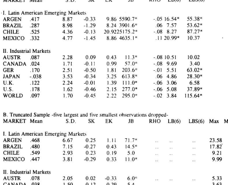
Table 1, Pane I A shows univariate statistics for the data. We note the usual high return-high

standard deviation characteristic of emerging markets. We test for normality using the Jarque-Bera

(1980) test, JB, which follows a chi-squared distribution with two degrees of freedom. Although for

both series normality is rejected by the 18. in emerging market<; the rejection is stronger. 5 This

stronger rejection arises mainly from higher kurtosis. Pane I A also shows the tirst autocorrelation

coefficient, RHO, and Ljung-Box (1978), LB(q), autocorrelation tests. The LB test follows a

chi-squared distribution with q degrees of freedom. The tirst order autocorrelation coefficient'i and the LB

tests, for mean returns, for both Latin American emerging markets and industrial markets are quite

similar, and, with the exception of Argentina and Mexico. there is no evidence for autocorrelation. For

4 McFarland, Pettit and Sung (1982) argue that week]y exchange rates also follow a non-normal

stable distribution. Therefore. since the hehavior of the fattest tai] dominates the tail behavior of a sum of variables, our tail estimates might capture the tai] hehavior of exchanges rates instead of local stock prices. We estimated the tail estimate in local currencies and the result<; were very similar to the results obtained in U.S. dollars. Later. we tested if the structural reforms enacted in the Latin American countries during our sample. affected the tai] estimate. These structural reforms have had a stabilizing influence on exchange rates. We could not. however. reject the null hypothesis of no change after the reforms.

..

the squared returns. however, the LB test reject<.; the no autocorrelation null hypothesis in ali the

markets with the exception of the U.K .. Australia.ó _{and Canada. Latin American emerging market<;}

. ·tend to show even higher squared autocorrelations. In Tahle I. Panel B. we analyze the impact of large

positive and negative observations in our sample hy Ieaving out 01' the analysis the tive largest and tive

smallest observations. Ali the industrial markets. with the exception 01' Japan and Australia, pass the

lB _{normality test, while among the Latin American emerging market<;. only Chile passes the} JB

normality test. The source 01' non-normalities in Argentina, Brazil. and Mexico does not seem to be

driven solely by a few extreme ohservations.

Table 2 focuses on the extreme ohservations In our sample. Four our purposes, extreme

observations are detined as observations which are outside 01' two standard deviations. Under

normality, the expected total numher should he around 17. Tahle 2 shows that the Latin American

emerging markets tend to have a lower total numher of extreme ohservations than the industrial

markets, although they are not statistically ditlerent. For portfolio managers, it would be useful to

know how clustered are these extreme ohservations. For example. a interesting question for portfolio

managers is: once an extreme ohservation has happened, is the prohability 01' ohserving another

extreme observation higher'! Tahle 2 also addresses this issue. Tahle 2 shows the number of single

extreme observations, where a single extreme ohservation is detined as an extreme observation not

followed or preceded by another extreme ohservation in four weeks. Again. with the exception of

Germany. this number is smaller for the emerging markets than for the industrial markets. This result

shows that the Latin American emerging markets tend to have the extreme ohservations more clustered

than the industrial markets. For example. in Argentina out 01' eighteen extreme ohservations only three

are single extreme ohservations. In contrast. in the U.K .. eleven extreme ohservations out 01' eighteen

•

are single extreme observations. Finally. the las! eigh! columns of Tahle 2 show the two largest

returns, the 95% percentile. the 90% percemile. the two smallest returns. the 5% percentile, and the

··10% percentile from each series. We find that. in ahsolute value. the two smallest returns tend to be

larger than the two largest returns. This hehavior of the extreme observations seems to reverse faster in

emerging markets than in industrial markets. as the percemile in Table 2 show. We also tind that the

two largest returns tend to be closer than the two smallest returns. Of particular relevance to investors

is the behavior of large negative returns. In the Latin American emerging markets, we tind that the

second smallest return is at least 40% larger than the minimum returno In industrial markets, however.

the second smallest return is on average 14% larger than the minimum returno We conclude that one of

the main differences between Latin American emerging markets and industrial markets is given by the

behavior of the returns on the tails of the distrihution. especially on the lower tai!.

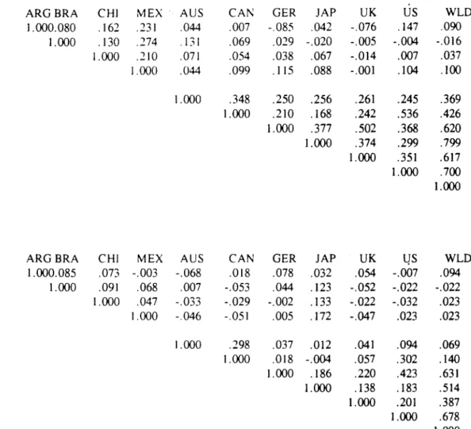
Table 3 shows the correlation matrix for returns and squared returns. Panel A, shows the typical

low correlation of stock returns in emerging markets and industrial market'\. The regional correlations

are on average larger than the correlations with developed markets. These low correlations are usually

interpreted as an indication of potential bendit for international portfolio diversitication. With few

exceptions. Pane I B. shows consistently lower correlations for squared returns. Engle and Susmel

(1993) show that higher correlations for the squared returns than correlations for the levei returns

might be indicating the existence of common time-varying component'\ in the variance. From that

perspective. the results in Pane I B show no evidence of common time-varying volatility in Latin

American emerging markets or in the industrial markets.

IV. TAIL ESTIMATES ANO THEIR IMPLlCATIONS TO INVESTORS

IV.A Tail estimates

•

lower tail. u_. and the common tai!. u. are rerorted in the first. second and third columns.

respectively. Below each point estimate. we report standard errors and the numher of order statistics

. 'used to estimate the tail indexo m .

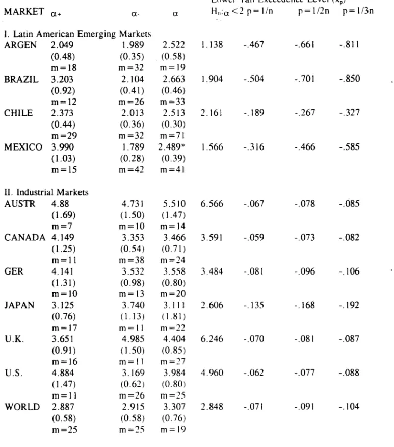
The lower tail tends to he fatter (smaller) than the uprer tai!. This is especially true for ali Latin

American emerging markets. With the exception of Mexico. the equality of hoth tails, however, cannot

be rejected. More important. hoth tails tend to he fatter for the Latin American emerging markets than

for the industrial markets. This result is true for the lower tail and common tai!. We also test for the

existence of second moments. If u is signiticantly lower than two, the equity returns do not have

second moments. The test is a one-sided test and follows a standard normal distrihution under the null

hypothesis. The null hypothesis is clearly rejected for industrial market<; and for Brazil and Chile. It

cannot be rejected for Mexico and Argentina.

We calculate exceedence leveis for ditlerent prohahilities. Recall that exceedence leveis are returns

that can only be achieved with a given prohahility. We use as prohahilities for the exceedence leveis

multiples of the inverse of the sample size. n

=

346. In the last three columns of Table 4 we report these calculations. For example, focusing on Argentina, the tifih column indicates that with probability

1/346 we can observe a negative return of -46.7 %. That is, in the Argentinean case, there is a 1 in 346

chance that an investor will oh serve a weekly return of -46.7% or less. Similarly, for Argentina, the

last column indicates that there is an almost .001 chance that an investor would experience a weekly

return of -81.1 % or less. From these last three columns. we ohserve that the exceedence leveis are

quite disperse from Latin American emerging markets. hut they are quite concentrated for industrial

markets.

We want to test the structural stahility of the tail estimates for Latin American equity markets.

These markets have experienced suhstantial deregulation and liheralization during the past six years.

we have enough observations to do a sensihle estimarion. For Argemina. the tail index is 2.63 before

liberalization and 2.99 after liheralization. For Brazil. the tail index is 2.60 hefore liheralization and

. '2.80 after liberalization. Even though rhere is a mild -decrease in the fatness of the tail, a formal test

cannot reject the equality of the indexes hefore and after economic reform. These results complement

previous results, using monthly data, that do nO[ ohserve any significam change in volatility, see De

Santis and lmrohoroglu (1995) and Bekaerr and Harvey (1995). However, they seem to contradict

Hargi-; (1994), who aIs o uses weekly stock returns for the same Latin American markets. Hargis

(1994) reports a decrease in volatility after liheralization.

IV. B Safety tirst porrfolio diversitkation

In this section, we study the diversitication possihilities which the Latin American emerging

markets afford a U.S. safety tirst investor. Assume that the U. S. investor is considering investing in a

Latin American portfolio. For simplicity, we use an equally weighted Latin American portfolio. In the

U.S., the investor can lend or horrow ar the risk-free rate. r. which we take as the weekly 9O-day

LIBOR.7 We construct 21 portfolios, increasing the percentage of the investment in the Latin American

portfolio fiom 0% to 100% hy increments of 5 % (for hrevity we do nO[ report ali the portfolios). As

pointed out hy JKV. the tail index. a. is unatlected hy forming these P ortfo li os , since the fattest tail

dominates the portfolio. In Tahle 5, however. we estimate ali the tail indexes for ali portfolios. As it

can be seen, for portfolios composed of 25 % or more of the Latin American portfolio, the lower tail

estimates are dominated hy the Latin American markets. i.e .. the tail index is close to two. For

portfolios composed of 20% or less of the Latin American porrfolio. the wntrihution of the Latin

American market'i is too small to dominate the U.S. Index. and therefore, the tail of the portfolio is

•

very similar to the U. S. tai I.

In order to study the implications of the safety first principie for the U.S. investor. we need to

"specify the parameter values of 8 and s. We assume that 8 takes on two values: .0029 (once every 6.7

years, or a 1 in 346 chance) and .0014 (a ! in 692 cham:e).' We use two conservative values of s: .9W

and .95W. For both leveIs of 8, the optima! investment in the Latin American portfolio is 15%, which

is a substantial reduction from the 50% reported in the introduction.9 _{The return on this risky portfolio}

is .002239% a week. The exceedence leveis for the safety first optima! risky portfolio are -.05.7 for

8=.0029 and -.072 for 8=.0014. Finally. we have 10 determine h, which depends on s. For exampIe,

for 8=.0029 and s=.95, h=-.128W. that is. the U.S. investor will he lending at the risk free rate

12.8% of her initial wealth. The return on the total portfo)jo is (.872 x 1.002239)

+

(.128 x 1.(01) = 1.00209. If the worst happens, the U.S. investor's tinal wealth is (.872 x .943)W

+

(.872 x

1.(02239)W = . 949W, or 95 percent of the initial wealth as expected.

V. CONCLUSIONS

In this paper, we analyze Latin American emerging market<; from a different perspective. We focus

on the tails of the unconditional distrihution of stock returns. We also explore the implications for

portfolio diversification of the safety tirst principie. First. we tind that the Latin American emerging

markets have signiticantly faner tails than industrial markets. This result is especially true for the

lower tail of the distrihution. Second, we consider a simple exercise to analyze the implication of the

safety first principIe for a U.S. investor who want<; to diversify his/her domestic portfolio using Latin

American market<;. For different parameter specitications, we tind that the safety tirst principie obtains

ｾ＠ We use different values for 8. The resu Its do not change suhstantially.

9 This percentage is consitent with the caps used in several glohal investment funds and with. the

TABLE 1. UNIVARIATE STATISTICS A. Full Sample

MARKET Mean S.O.

.. I. Latin American Emerging Markets

SK EK 18

ARGEN .417 8.87 -0.33 9.86 5590.7*

BRAZIL .287 8.98 -1.29 8.24 3901.6*

CHILE .525 4.36 -0.13 20.9225175.2*

MEXICO .332 4.77 -1.45 8.864635.1*

11. Industrial Markets

AUSTR .087 2.28 0.09 0.43 11.3*

CANADA .024 1. 71 -0.11 0.99 57.0*

GER .170 2.51 -0.50 1.81 203.6*

JAPAN -.038 3.53 -0.34 3.25 613.8*

U.K. .122 2.24 -0.01 1.39 111.0*

U.S. .178 1.62 -0.46 2.15 277.0*

WORLO .097 1.70 -0.45 2.22 295.0*

RHO LB(6) LBS(6)

-.05 16.54* 55.38* .06 7.57 53.62* -.08 8.27 87.27* .11 20.99* 10.37

-.08 10.51 10.02 -.08 9.69 3.40 -.01 5.51 63.02*

.06 4.86 28.30* -.06 3.06 6.58 -.06 5.08 37.89* -.02 3.84 115.64*

B. Truncated Sample -tive largest and tive smallest ohservations

dropped-MARKET Mean S.O. SK EK 18 RHO LB(6) LBS(6) Max Min

I. Latin American Emerging Markets

ARGEN .468 6.67 0.25 1.1 I

BRAZIL .480 7.15 -0.27 0.43

CHILE .549 2.93 0.23 0.19

MEXICO .447 3.81 -0.29 0.33

11. Industrial Markets

AUSTR .078 2.05 0.02 -0.33

CANADA .038 1.50 0.12 0.29

GERM .196 2.18 -0.28 0.01

JAPAN -.022 2.95 -0.23 0.46

U.K. .119 1.96 -0.10 0.11

U.S. .145 1.40 -0.16 0.09

WORLO .105 1.46 -0.30 0.10

Notes:

* signiticant at the 5 % leveI. SK: Skewness coeftlcient. EK: Excess kurtosis coefticient. JB: Jarque-Bera (1980) normality test. RHO: First order autocorrelation coefticient. LB(6): Ljung-Box statistic with 6 lags for leveis.

71.7* 14.5* 5.0 11.0* 6.0'" 5.4 4.4 14.6* 1.2 1.1 5.6

LBS(6): Ljung-Box statistic with 6 lags for squareu series.

23.58 -19.35 17.82" -22.68 9.21 -8.20 9.99 -12.14

TABLE 2. EXTREME OBSERVATIONS

MARKET Total ｓｩｬｬｾｊ･＠ m .. x! m;,x.:::' llldX) f/f 1l1;'x!O',; minlO';7 min5'ii min.:::' minI

L Latin American Emerging Markets

.. ARGEN 18 3 42.84 41.02 12:18 8.57 -8.08 -11.99 -32.12 -61.75

BRAZIL 15 4 31.32 27.52 13.28 10.11 -9.58 -13.47 -38.24 -66.81 CHILE 11 4 33.79 18.71 6.18 4.62 -3.33 -4.50 -18.40 -33.40 MEXICO 17 5 14.57 13.44 7.39 5.69 -4.64 -6.45 -18.74 -34.54

11. Industrial Markets

AUSTR 18 6 8.24 6.17 3.85 2.98 -2.84 -3.91 -6.21 -7.12

CANADA 16 12 5.58 4.95 2.95 2.28 -2.07 -2.54 -6.16 -6.27

GER 16 4 8.10 7.49 3.87 3.02 -2.87 -4.39 -8.55 -11.74

JAPAN 20 7 14.92 10.94 5.56 3.96 -3.88 -6.32 -12.37 -18.06

U.K. 18 11 8.62 8.04 3.83 2.59 -2.71 -3.93 -6.34 -7.99 .

U.S. 19 9 5.70 4.31 2.91 2.18 -1.90 -2.69 -5.72 -7.82

WORLD 19 6 5.28 5.23 2.72 2.01 -2.14 -2.76 -4.88 -8.51

Notes:

Total: total number of observations larger (in absolute value) than two standard deviations.

Single: number of extreme ooservations not followed nor preceded oy another extreme observation in four weeks.

max 1: largest observation.

max2: second largest observation.

max5 %: 5 % fractile of the 1argest observatiol1s. max 10%: 10% fractile of the largest observations. minI: smallest observation.

min2: second smallest observation.

TABLE 3. CORRELATIOl'\ MATRIX

A.- Leveis

ARG BRA CHi MEX AUS CAl\: GER JAP UK US WLD

ARGENTINA 1.000.080 .162 .231 .044 .007 -.085 .042 -.076 .147 .090

\ _{BRAZIL i.OOO .130 .274 .131 .069 .029 -.020 -.005 -.004 -.016}

CHILE 1 .000 .210 .071 .054 .038 .067 -.014 .007 .037

MEXICO 1 .000 .044 .099 .115 .088 -.001 .104 .100

AUSTRALIA 1.000 .348 .250 .256 .261 .245 .369

CANADA 1.000 .210 .i68 .242 .536 .426

GERMANY 1.000 .377 .502 .368 .620

JAPAN 1.000 .374 .299 .799

U.K. 1.000 .351 .617

U.S. 1.000 .700

WORLD 1.000

B.- Squared Series

ARGBRA CHI MEX AUS CAN GER JAP UK l!S WLD

ARGENTINA i.OOO.085 .073 -.003 -.068 .018 .078 .032 .054 -.007 .094

BRAZIL 1.000 .091 .068 .007 -.053 .044 .i23 -.052 -.022 -.022

CHILE i.OOO .047 -.033 -.029 -.002 .133 -.022 -.032 .023

MEXICO 1.000 -.046 -.051 .005 .i72 -.047 .023 .023

AUSTRALIA 1.000 .298 .037 .012 .041 .094 .069

CANADA 1.000 .018 -.004 .057 .302 .140

GERMANY 1.000 .186 .220 .423 .631

JAPAN 1.000 .138 .183 .514

U.K. 1.000 .201 .387

U.S. 1.000 .678

TABLE 4. TAIL ESTIMATES A. FulI Sample

Lower Tail Exceedence LeveI (xp)

MARKET _{u+ a- a} H,,:a <2 p= IIn p = 1/2n p = 113n

•

I. Latin American Emerging Markets

ARGEN 2.049 1.989 2.522 1.138 -.467 -.661 -.811

(0.48) (0.35) (0.58)

m=18 m=32 m=19

BRAZIL 3.203 2.104 2.663 1.904 -.504 -.701 -.850

(0.92) (0.41) (0.46)

m=12 m=26 m=33

CHILE 2.373 2.013 2.513 2.161 -.189 -.267 -.327

(0.44) (0.36) (0.30)

m=29 m=32 m=71

MEXICO 3.990 1.789 2.489* 1.566 -.316 -.466 -.585

(1.03) (0.28) (0.39)

m=15 m=42 m=41

11. Industrial Markets

AUSTR 4.88 4.731 5.510 6.566 -.067 -.078 -.085

(1.69) ( 1.50) (1.47)

m=7 m=1O m=14

CANADA 4.149 3.353 3.466 3.591 -.059 -.073 -.082

( 1.25) (0.54) (0.71 )

m=11 m=38 m=24

GER 4.141 3.532 3.558 3.484 -.081 -.096 -.106

(1.31) (0.98) (0.80)

m=1O m=13 m=20

JAPAN 3.125 3.740 3.111 2.606 -.135 -.168 -.192

(0.76) (1. 13) (1.81 )

m=17 m=11 m=22

U.K. 3.651 4.985 4.404 6.246 -.070 -.081 -.087

(0.91) ( 1.50) (0.85)

m=16 m=11 m=27

U.S. 4.884 3.169 3.984 4.960 -.062 -.077 -.088

(1.47) (0.62) (0.80l

m=11 m=26 m=25

WORLD 2.887 2.915 3.307 2.848 -.071 -.091 -.104

(0.58) (0.58) (0.76)

m=25 m=25 m=19

Notes:

T ABLE 5. Lower tail estimates for Ditferent PllrttO!iOS

Proportion of Exceedem:e Leveis and Returns

• LA in port a. SE(a.) m XIi .m 1)= 1/11 (R-r)/(r-q)8 = 1/2n (R-r)/(r-q)

..

'·0% 3.169 0.622 26 -0.022-.062 .0146 -.077 .0118

5% 2.991 0.556 29 -0.020-.061 .0166 -.077 .0133

10% 2.945 0.676 19 -0.022-.059 .0188 -.074 .0149

15% 3.070 0.704 19 -0.022-.057 .0211 + -.072 .0169+

20% 2.884 0.721 16 -0.024-.063 .0201 -.080 .0166

25% 2.145 0.405 28 -0.018-.085 .0167 -.118 .0121

30% 2.183 0.476 21 -0.022-.089 .0171 -.123 .0124

40% 2.339 0.585 16 -0.030-.098 .0177 -.131 .0132

50% 1.969 0.464 18 -0.031-.135 .0144 -.192 .0101

60% 1.725 0.396 19 -0.033-.182 .0118 -.272 .0079

70% 1.747 0.276 40 -0.025-.209 .0113 -.311 .0076

75% 1.818 0.291 39 -0.028-.212 .0116 -.310 .0079

80% 1.632 0.385 18 -0.044-.257 .0100 -.394 .0065

85% 1.641 0.398 17 -0.048-.272 .0098 -.415 .0064

90% 1.834 0.315 34 -0.037-.252 .0110 -.368 .0075

95% 1.774 0.292 37 -0.037-.280 .0103 -.414 .0069

100% 1.680 0.269 39 -0.036-.322 .0093 -.486 .0061

Notes:

+:

preferred ponfolio .

•

•

..

References

Arzac, E.R. and V.S. Bawa (1977). "Portfolio Choice and Equilihrium in Capital Markets with Safety-First Investors," Journal of Financiai Ecol1omics. 4. 277-288 .

Baillie, R.T. and R.P. DeGennaro (1990). "Stllck Returns and Volatility." Journal of Financia'l and Ouantitative Analysis, 25. 203-214.

Bekaert, G. and C.R. Harvey (1995). "Time-Varying World Market Integration." Journal of Finance, 50, 403-444.

Bekaert, G. and C.R. Harvey (1996). "Emerging Equity Market Volatility," Department of Finance. Duke University, manuscript.

Blattberg, R.C. and N.J. Gonedes (1974). "A Comparison of the Stahle and Student Distribution as Statistical Models for Stock Prices," Journal of Business. 244-280.

Bollerslev, T.P. (1987), "A Conditional Time Series Model for Speculative Prices and Rates of Returns," Review of Economics and Statistics. 69. 524-54.

Cho, D.C, C.S. Eun and L.W. Senhet (1986). " lnternatiol1al Arhitrage Pricing Theory: An Empirical Investigation," Journal ofFinance, 41. 313-329.

Chuhan, P. (1992), "Sources of Portfolio Investment in Emerging Markets." manuscript.

Claessens, S., S. Dasgupta and l. Glen (1995). "Return Behavior in Emerging Stock ｍ｡ｲｫ･ｴｾＮＢ＠ World Bank Economic Review, 9. 131-15 I .

De Santis, G. (1993), "Asset Pricing and Portfolio Diversitication: Evidence from Emerging FinanciaI Markets," Department of Finance and Business Economics. University of Southern California, unpublished manuscript.

De Santis, G. and S. Imrohoroglu (1995). "Stock Returns and Volatility in Emerging Financiai Markets," Department of Finance and Business Economics. lJniversity of Southern California, unpublished manuscript.

Engle. R.F. and R. Susmel (1993). "Col11l11on Volatilitv In International Equity Markets." Journal of

Business and Economic Statistics. 11.2. 167-176.

Fama, E. (1965), "The Behavior of Stock Market Prices." lournal of Business. 38. 34-105.

Goldie C.M. and R.L. Smith. "Slow Variation with Remainder: Theory and Applications," Ouarterly Journal of Mathematics. 38. 45-71.

•

•

..

•

Hargis, K. (1994), "Time-Varying Transm ission of Priees ano V olatil it)' Latin American Equity Markets 1988-1994." Department of Eeonomies. University of IlIinois at Urhana-Champaign. unpublished manuscript.

··Harvey, C.R. (1993), "Portfolio Enhaneement with Emerging Markets and Conditioning lnformation," in S. Claessens and S. Gooptu (eds.): Portfolio Investment in Developing Countries, World Bank, Washington, D.C.

Harvey, C.R. (1994), "Conditional Asset Alloeation in Emerging Markets." Departmem of Finance, Duke University, manuscript.

Harvey, C.R. (1995a), "Predictable Risk and Returns In Emerging ｍ｡ｲｫ･ｴｾＮＢ＠ Review of FinanciaI Studies, 8, 773-816.

Harvey, C.R. (1995b), "The Risk Exposure of Emerging Equity Market<;," World Bank Economic Review, 9, 19-50.

Hill, B.M. (1975) " A Simple General Approaeh to Inferenee Ahout the Tail of a Distribution," The Annals of Statistics, 3, 1163-1173.

Hols, M. and C.G. de Vries (1991), "The Limiting Distrihution of ExtremaI Exchange Rate Returns," Journal of Applied Econometrics. 287-302.

Jansen, D.W.and C.G. de Vries (1991), "On the Frequency of Large Stock Returns: Puning Booms and Busts imo Perspective, " The Review of Economies and Statistics, 18-24.

Jansen, D.W., K.G. Koedijk, and c.G. oe Yries (1996). "Operationalizing Safety First Portfolio Selection using Extreme Value Theory." Department of Economics. Texas A&M University, manuscript.

Koedijk, K.G, M.M.A. Schafgans and c.G oe Vries (1990). "The Tail lndex of Exchange Rate Returns," Journal of lnternational Econom ies. 19. 93-108.

Leadbener, M.R .. G. Lindgren and H. Rootzen (1983). Extreme and Related Properties of Random Sequences and Processes. Berlin. Germany: Springer-Yerlag.

Longin, F. (1993). "Booms and Crashes: Appliearion of Extreme Value Theory to the U.S. Stock Market," London Business Sehoo\. manuseript.

Loretan, M. and P.C.B. Phillips (1994). "Testing the Covarianee Stationarity of Heavy-Tailed Time Series: An Overview of the Theory With Applieations to Severa I FinanciaI Datasets." Journal of Empirical Finance, 1. 211-248.

Mandelbrot. B.B. (1963), "The Variation llfCertain Speeulative Prices." Journal ofBusiness, 36,

394-419. .

•

Changes: Trading Day Effects and Risk Measurement." lorunal ot Finance. 38. 693-715.

Roy, A.D. (1952), "Safety First and the Ho1ding of Assets." Econometrica. 431-449 .

•

ｾ＠ . Tesar, L. and LM. Werner (1994). "International Securities Transaction and U.S. Portfolio Choice,"

li

in The Internationalization of Equit), Markets. Chicago. 111.: The University of Chicago Press.

FUNDAÇÃO GETULIO VARGAS

BIBLIOTECA

ESTE VOLUME DEVE SER DEVOLVIDO A BIBLIOTECA NA ÚLTIMA DATA MARCADA

ｾＮ＠ '''' I

l\.Cham. P/EPGE SPE S964ex

Autor: Susmel, Raul.

Título: Extreme obsenations and di\'ersificatlon in Latin

1111111111111111111111111111111111111111

086183

49993

FGV - BMHS NU 1'''1.1'84,98

"