Extreme value theory in emerging markets

(1)

UDC: 3.33 ISSN: 0013-3264

SCIENTIFIC PAPERS

* Faculty of Technical Sciences, Department for Industrial Engineering and Management,

Novi Sad, Serbia, gandjelic@uns.ac.rs, ivanamilosev@yahoo.com, v_djakovic@uns.ac.rs JEL CLASSIFICATION: D81, G10, G11

ABSTRACT:_{his paper investigates the} performance of extreme value theory (EVT) with the daily stock index returns of four diferent emerging markets. he research covers the sample representing the Serbian (BELEXline), Croatian (CROBEX), Slovenian (SBI20), and Hungarian (BUX) stock indexes using the data from January 2006 – September 2009. In the paper a performance test was carried out for the success of application of the extreme value theory in estimating and forecasting of the tails of daily return distribution of the analyzed stock indexes. herefore the main goal is to determine whether EVT adequately estimates and forecasts the tails (2.5% and 5% at the tail) of daily stock

index return distribution in the emerging markets of Serbia, Croatia, Slovenia, and Hungary. he applied methodology during the research includes analysi s, synthesis and statistical/mathematical methods. Research results according to estimated Generalized Pareto Distribution (GPD) parameters indicate the necessity of applying market risk estimation methods, i.e. extreme value theory (EVT) in the framework of a broader analysis of investment processes in emerging markets.

KEY WORDS:_{Extreme Value heory,} Value at Risk, Risk Management, Generalized Pareto Distribution, Emerging Markets

DOI:10.2298/EKA1085063A

Goran Andjelic,

Ivana Milosev,

and Vladimir Djakovic*

(2)

1. INTRODUCTION

The modern terms of business activities in the financial markets condition the application of suitable methods of risk management. Events such as the financial crisis and financial market crash point to the inevitability of quantification and the estimation of the probability of occurrence of extremely high losses in investment activities. Currently Value at Risk (VaR) represents the most popular method of quantification and market risk management. Market risk is defined as the result of the price change of securities on the capital markets (Bessis, 2002).

The financial instability in the early 1970s generated the need for quantification of the market risks of the most important financial institutions. VaR was published by J P Morgan in 1994 as the method of risk management behind its Risk Metrics system. Theoretical ground for the VaR method was given by Jorion (1996), Duffie and Pan (1997) and Dowd (1998). It is defined as the worst loss over a target horizon with a given level of confidence (Jorion, 2001). VaR is a statistical measure of the maximal losses that can be incurred in investment activities, and losses that surpass the value of the VaR happen only with a certain probability (Linsmeier et al., 2000).

(3)

assets such as volatility, kurtosis, and skewness are significant asset return characteristics.

The most common criticism, that the assumption that the profits/losses on a portfolio are normally distributed, is unrealistic. The theoretical ground that was provided by Mandelbrot1,2_{shows that financial return series exhibit} leptokurtosis or 'heavier tails' than a normal distribution (Hauksson et al., 2000; Dacorogna et al., 2001). In essence, this means that any VaR calculation technique based on a normal distribution function will tend to give VaR estimates that are too low (Seymour and Polakow, 2003). Assuming normality when our data are heavy-tailed can lead to major errors in our estimates of VaR. Thus VaR will be underestimated at relatively high confidence levels and overestimated at relatively low confidence levels (Obadovic and Obadovic, 2009: 135).

Beyond the traditional approaches there is an alternative that uses the Extreme Value Theory (EVT) to characterize the tail behaviour of the distribution of returns. By focusing on extreme losses the EVT successfully avoids tying the analysis down to a single parametric family fitted to the whole distribution. Embrechts et al. (1997) and Mc-Neil and Fray (2000) survey the mathematical foundations of EVT and discuss its applications to financial risk management. The empirical results show that EVT-based models provide more accurate VaR estimates, especially in higher quantiles (Embrechts et al., 1999). For example, McNeil (1997), Harmantzis and Miao (2005) and Marinelli et al. (2007) show that EVT outperforms the estimates of VaR based on analytical and historical methods.

A special challenge is represented by the exploration of the possibilities of application, i.e. the performance of extreme value theory (EVT) on the financial markets of emerging countries, i.e. emerging markets. In the literature of the

1 _{Mandelbrot, B. (1963), ‘New methods in statistical economics’,}_{Journal of Political Economy}_,

Vol. 71, No. 5, pp. 421 – 440.

2 _{Mandelbrot, B. (1963), ‘The variation of certain speculative prices’,}_{Journal of Business}_{, Vol.}

(4)

subject matter a fundamental difference exists between developed and emerging markets. Generally viewed, the world`s most developed stock exchange markets are considered more liquid and more efficient compared to those still emerging. In emerging markets such as Serbia there is also the case of a small number of data points (Drenovak and Urosevic, 2010).

The application of the EVT to emerging markets requires special attention, especially regarding insufficient liquidity, the small scale of trading, and, historically speaking, the asymmetrical and low number of trading days with certain securities. Financial theory indicates that higher volatility, which is characteristic for the returns of emerging markets, corresponds to higher expected returns on those markets (Salomons and Grootveld, 2003). Time series on financial markets often have the following characteristics: changing variability during time and empirical distribution that has tails that are heavier than tails of the normal distributions (Mladenovic and Mladenovic, 2006: 33). Also, compared to developed markets, emerging markets are characterized by capital market reforms, frequent internal and external financial shocks, a high level of country risk (i.e. political risk, economic risk, and financial risk), changes in credit rating, fluctuation of foreign exchange rates, a high level of insider trading, etc. Consequently economic activity in transition economies affected by the global crisis deteriorated much faster, from slowdown to rapid decline (Nuti, 2009). The previously listed factors considerably influence the increase of market volatility and consequently result in the increase of the divergence from normal distribution, which results in the impossibility to adequately predict the market risk, i.e. the emergence of extreme values in investment activities.

(5)

Croatian (CROBEX), Slovenian (SBI20), and Hungarian (BUX) stock indexes. EVT provides a formal framework for the study of the left and right tail behaviour of the fat-tailed return distributions. Namely, risk and reward are not equally likely to occur in these emerging markets.

The central objective of this paper is to test the performance of the application of the EVT on return series generated by the given stock indexes. Therefore the main motivation of this research is to provide up-to-date evidence on the risk management and return characteristics of emerging markets over time, i.e. to enable better forecast of out-of-sample events. Results of this research will be especially interesting to both domestic and foreign investors in global recessive business conditions. We present empirical evidence of the performance of application of the EVT in the emerging markets of the selected Central and Eastern European countries.

2. THEORETICAL BACKGROUND

The statistical analysis of extremes is essential for many of the risk management problems related to finance, i.e. investment processes. Extreme value theory (EVT) is the study of the tails of distributions and it is the key for sound risk management of financial exposures. Namely, forecast of the extreme movements that can be expected in financial markets, especially emerging ones, is tested within the framework of the EVT. The basic idea behind extreme value theory (EVT) is that in applications where only large movements are taken into consideration in some random variable, it may not be optimal to model the entire distribution of the event with all available data. Instead it may be better only to model the tails with tail events. Extreme value theory is a theory of the behaviour of large or extreme movements in a random variable, where extreme observations are used to model the tails of a random variable.

(6)

Definition 1. Let

 

n i i

X _₁ be a set of independent and identically distributed random variables with distribution function



X x



P x

F( ): i  (1)

for any i. Also, we have to be able to assess the upper and lower tails of the distribution function F. Thus, consider the order statistics



n



n X X X

M max ₁, ₂,..., and mnmin



X1,X2,...,Xn



.

Both Mn and mn are random variables that depend on the length n of the sample. Analogically with the Central Limit Theorem, we will be interested in the asymptotic behavior of these random variables as n→∞. Since



n



n X X X

m max  ₁, ₂,..., , it is sufficient to state all the results for Mn, that is, focus on observations in the upper tail of the underlying distribution. The results for the lower tail will be straightforward to generalize.

The following theorem is a limit law first derived heuristically by Fisher and Tippett 3_{, and continued later by Gnedenko}4_.

Theorem 1. Let

 

n i i

X _₁ be a set of n independent and identically distributed random variables with distribution function F and suppose that there are sequences of normalization constants,

 

an and

 

bn , such that, for some non-degenerated limit distribution F*_{, we have}







F a x b



F  x x

a b M

P n n n

n n n n n * lim

lim _  

         

 ,xR (2)

Then, there exist R,R and Rsuch that F  x ,, x

* __

for any R

x , where

3 _{Fisher, R.A. and L.H.C. Tippett (1928), ‘Limiting Forms of the Frequency Distribution of the}

Largest or Smallest Member of a Sample’, Proceedings of the Cambridge Philosophical Society, Vol. 24, pp. 180 – 190.

(7)

 

_



X x



x

F  



X X X



M  



X X X





X X X



 

 

_

 











              

 x

        x

  _            _           _ 

 1/

,

, : exp 1

x

x (3)

is the Generalized Extreme Value (GEV) distribution, which was first proposed in this form by von Mises5_{. The}₁_/_{is referred to as the tail index, as it} indicates how heavy the upper tail of the underlying distribution F is. When

0



 , the tail index tends to infinity and ,, x exp



exp







x



/





.

Embrechts et al. (1997) describe GEV distribution in detail. Three fundamental types of extreme value distributions are defined by :

1) If  0, the distribution is called the Gumbel distribution. In this case, the distribution spreads out along the entire real axis.

2) If  0, the distribution is called the Fréchet distribution. In this case, the distribution has a lower boundary.

3) If  0, the distribution is called the Weibull distribution. In this case, the distribution has an upper boundary.

The Fisher and Tippett theorem suggests that the asymptotic distribution of the maxima belongs to one of the three distributions above, regardless of the original distribution of the observed data. Random variables fall into one of three tail shapes, fat, normal, and thin, depending on the various properties of the distribution. Thus, the tails of distributions are:

- Thin. i.e. the tails are truncated.

- Normal. In this case, the tails have an exponential shape. - Fat. The tails follow a power law.

It is a fact that financial returns are fat. The upper tail of any fat-tailed random variable (x) in EVT has the following property:

5 _{Von Mises, R. (1936), ‘La Distribution de la plus grande de n Valeurs’ in Selected Papers II.}

(8)

           x t F tx F t 1 1

lim , α>0, x>0 (4)

where α is known as the tail index, and F (•) is the asymptotic distribution

function. The reason why this is important is that, regardless of the underlying distribution of x, the tails have the same general shape, where only one

parameter is relevant, i.e. α.

Theorem 2. Let

 

n i i

X _₁ be a set of n independent and identically distributed

random variables with distribution function F. Define

 









 

 u F u F y u F u X y u X P y F_u         1

: , y>0 (5)

as the distribution of excesses of X over the threshold u. Let xF be the end of the upper tail of F, possibly a positive infinity. Then, if F is such that the limit given by Theorem 1 exists, there are constants Rand Rsuch that

    0

sup

lim  _,  

 

x _u _x _x Fu x G x u u

F F



 , (6)

where

 

    _ / 1

, : 1 1

        _   y y

G (7)

is known as the Generalized Pareto Distribution (GPD).

The application of EVT involves a number of challenges. First, the parameter estimates of the Generalized Extreme Value (GEV) distribution and GP limit distributions will depend on the number of extreme observations used. Second, the choice of a threshold should be large enough to satisfy the conditions that permit the application of Theorem 2, i.e. uxF, while at the same time leaving

(9)

 

  

 

  

F x

(•) is the asymptotic distribution function. The reason why this is important is that, regardless of the underlying distribution of , the tails have the same general shape, where only one parameter is relevant, i.e. α.

 

_ be a set of n independent and identically distributed random variables with distribution function F. Define

 









    y       

 _{, y>0} ₍₅₎

as the distribution of excesses of X over the threshold u. Let xF be the end of the upper tail of F, possibly a positive infinity. Then, if F is such that the limit given by Theorem 1 exists, there are constants   _such that

   

sup   

   

 

    _         _  

is known as the Generalized Pareto Distribution (GPD).

The application of EVT involves a number of challenges. First, the parameter estimates of the Generalized Extreme Value (GEV) distribution and GP limit distributions will depend on the number of extreme observations used. Second, the choice of a threshold should be large enough to satisfy the conditions that permit the application of Theorem 2, i.e. x

a sufficient number of observations to render the estimation feasible (Bensalah, 2000).

Da Silva and de Melo Mendez (2003), Danielsson and de Vries (1997) and Embrechts et al. (1997) overviewed several empirical methods for estimation of tail thickness. The primary difficulty in estimating the tails is the determination of the start of the tails. Characteristically, these estimators use the highest/lowest realizations to estimate the parameter of tail thickness, which is called the tail index. The moments based estimator for the tail index was proposed by Hill.6 The estimator is conditional on knowing how many extreme order statistics for a given sample size have to be taken into account. The tail index is estimated by using the most extreme observations above a threshold Sn, where n is the sample size. The most common estimator of the tail index is the Hill estimator, which is generally considered to have more desirable properties than other estimators. The efficient determination of the tail threshold, Sn, requires an optimal assessment of the trade–off between bias and variance (Danielsson and de Vries, 2002).

In our study the performance of EVT is analyzed in emerging markets of the selected Central and Eastern European countries. Zikovic and Aktan (2009) investigated the relative performance of a wide array of VaR models with the daily returns of the Turkish and Croatian stock index. They concluded that only advanced and theoretically sound VaR models such as EVT and HHS can adequately measure equity risk on the Turkish and Croatian equity markets in times of crisis. Similarly Gencay and Selcuk (2004) examined the relative performance of VaR models with the daily stock market returns of nine different emerging markets. Coronel-Brizio and Hernandez-Montoya (2005) investigated the so-called Pareto-Levy or power-law distribution as a model to describe probabilities associated with extreme variations of worldwide stock market indexes data. Embrechts et al. (1999) examined the role of extreme value theory as an important methodological tool for securitization of risk and alternative risk transfer. Da Silva and de Melo Mendez (2003) used the extreme value theory to analyze ten Asian stock markets, identifying which type of extreme value asymptotic distribution better fits historically extreme market events. They concluded that the extreme value method of estimating VaR is a

(10)

more conservative approach to determining capital requirements than traditional methods. Mladenovic and Mladenovic (2006) investigated and exhibited the evaluation of value parameters regarding risk based on analysis of the specific financial time series. They investigated the daily return data of share prices of CISCO and INTEL companies as well the NASDAQ market index, and concluded that one of the key elements in application of the extreme value theory is determining a threshold value, and consequently a group of extreme values. Drenovak and Urosevic (2010) investigated the Serbian market using the Svensson parametric model, taking into account issues specific to emerging markets in general and the Serbian market in particular. They argue that no risk management or asset/liability model, the cornerstones of the contemporary financial industry, can be implemented without regular use of benchmark spot curve estimates.

The contribution of this paper is the empirical investigation and analysis of extreme value theory (EVT) on the daily stock index returns of four different emerging markets, while estimating and forecasting the tails of the daily return distribution of the tested stock indexes.

3. METHODOLOGY REVIEW

This part of the paper presents the research methodology that is particularly focused on the performance analysis of the application of the extreme value theory (EVT) on the emerging markets of Serbia, Croatia, Slovenia and Hungary, i.e. in investment activities. Volatile markets provide an appropriate environment to study the performance of the EVT. The high volatility and thick-tail nature of the Serbian (BELEXline), Croatian (CROBEX), Slovenian (SBI20), and Hungarian (BUX) stock indexes provide an adequate platform to test the performance of application of the extreme value theory (EVT) in the emerging markets of selected Central and Eastern European countries.

(11)

(12)

The returns on the stock indexes tested in this paper are calculated as





1 ln 1

ln

   

t t t

t

P P R

r (8)

where

Rt – return on stock index during a period t, Pt – stock index price during a period t, Pt-1 – stock index price during a period t-1.

The changes in the daily returns of the stock indexes point to the specificities, i.e. characteristics of the observed emerging markets with a special accent on investment possibilities and market risks as the determinants of such activities. With the analysis of the success of the Generalized Pareto Distribution (GPD), the behaviour of the emerging markets is tested in terms of volatility and probability of extreme value occurrences. The in-sample period comprises the period between 10.01.2006 and 31.08.2007, while the out-of-sample period comprises the period between 01.01.2008 and 31.08.2009. On the basis of the in-sample period the threshold value was calculated, according to which the returns value of the following day was tested. The returns value was successfully estimated in case the returns value of the following day was higher than the estimated value for the left tail and less than the estimated value for the right tail. For the opposite the estimation was unsuccessful.

(13)





   

416th_{data points to obtain a forecast of the 417}th_{day return with updated} parameters from this new sample.

The second approach understands an interval of 415 days, in such a way that the interval is increased after testing each of the following days, and which is added to the in-sample without casting out the oldest daily returns (long interval). In this way the number of the days is increased, according to which the model estimation and the daily return forecast is carried out. That is, this approach does not utilize a window and uses all available data starting at the 415th_{day. For} instance, the model is estimated adding the 416th_{day return into the sample and} a forecast of the 417th_{day return is obtained and stored. Since it is practically} impossible to determine an optimum parameterization or a threshold value for each approach (optimal threshold determination), i.e. instead of determining a threshold value at each step, we utilized 2.5% and 5% at the tail of the observed sample in both GPD approaches. At the beginning of the analysis the distribution of the sample has been tested with the Kolmogorov-Smirnov test, with the objective of determining whether the sample has normal distribution. On the basis of the central dispersive parameters, the picture of the distribution of the sample was gained. The normal distribution of the sample means that the coincidental variable (x), with the arithmetical middle μ and the standard deviation σ, is normally distributed in case the function of probability f (x) gives the variable (x) the value of X, following the next function of probability:

 





_

  

 

   

   

 2

2 1 exp 2 1

  



x x

f (9)

where

(14)

Also, during the testing of the sample, its characteristics have been examined - skewness and kurtosis. Their coefficients have been calculated according to the next formulae:

Coefficient skewness =





 

3 1

n n

i

n i

S X X n



_ 

(10)

Coefficient kurtosis =





 

₂ 2 1

4 1

n n

k

n i

S X X n



_ 

(11)

where

i

X - sample, n

X - middle of the sample, n

S - dispersion of the sample.

The Kolmogorov–Smirnov test is used to test whether two underlying one-dimensional probability distributions differ. The random process F(x) is formed as the estimation problem and q used as the test statistic:

q = x

max |Fˆ (x) - F0 (x)| (12)

This choice is based on the following observations: For a specific ζ, the function

Fˆ (x) is the empirical estimate of (x). It tends, therefore, to F(x) as n→∞. From

this it follows that:

E(Fˆ (x))=F(x) Fˆ (x) → F(x), (n → ∞ ) (13)

This shows that for large n, q is close to 0 if H0 is true and it is close to F(x) –

F0(x) if H1 is true. It leads, therefore, to the conclusion that we must reject H0 if

(15)





 



 





 



 

X

significance level α = F {q > c|H0}and the distribution of q. Under hypothesis

H0, the test statistic q is used. Using the Kolmogorov approximation, we obtain:





₂ 2

0 1 e nc

H c q

P    



 (14)

The test thus proceeds as follows: Form the empirical estimate Fˆ (x) of F(x);

Accept H0if

2 ln 2

1 

n

q  (15)

The resulting Type II error probability is reasonably small only if nis large.

The research carried out in the paper understands the analysis of the performances of the named calculation approaches of the GPD in the selected emerging markets, i.e. the adequacy of the usage of the limited or the long interval. Due to the previously mentioned characteristics of emerging markets in the introduction to the paper, it was not possible to apply a standard approach to this problem, when for the in-sample period a fixed period of a different number of days was taken. Namely, there is simply not enough data to do sensible analysis in the selected emerging markets, whether by EVT or any other method. The global economic crisis represents a special problem, which especially started to manifest itself in the observed emerging markets from September 2008, which additionally influenced the shortening of the period in which the results of the application of the EVT could be analyzed.

4. DATA AND PRELIMINARY ANALYSIS

(16)

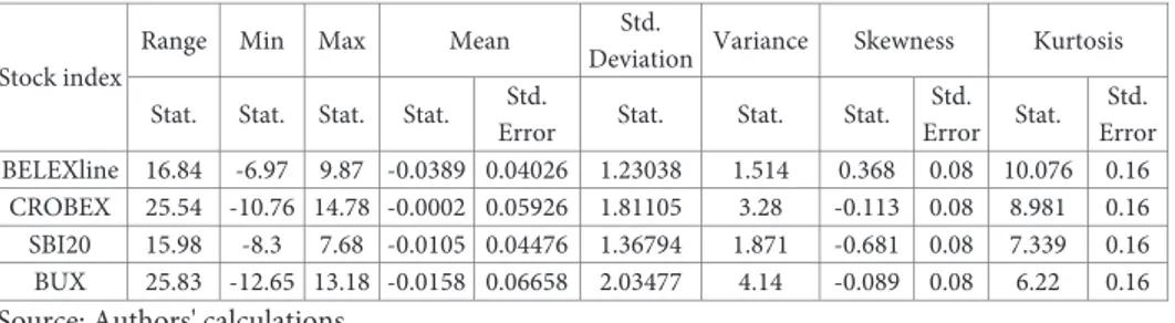
Table 1 provides descriptive statistics of daily returns, computed as





1 ln 1

ln

   

t t t

t

P P R

r . Daily sampling is chosen in order to capture high-frequency fluctuations in return processes that may be critical for identification of rare events in the tails of distribution, while avoiding modeling the intraday return dynamics, abundant with spurious emerging market microstructure distortions and trading frictions.

Table 1. Descriptive statistics of the daily returns in the period 10.01.2006 – 31.08.2010 (934 days)

Stock index

Range Min Max Mean Std.

Deviation Variance Skewness Kurtosis

Stat. Stat. Stat. Stat. Std.

Error Stat. Stat. Stat. Std. Error Stat.

Std. Error BELEXline 16.84 -6.97 9.87 -0.0389 0.04026 1.23038 1.514 0.368 0.08 10.076 0.16

CROBEX 25.54 -10.76 14.78 -0.0002 0.05926 1.81105 3.28 -0.113 0.08 8.981 0.16 SBI20 15.98 -8.3 7.68 -0.0105 0.04476 1.36794 1.871 -0.681 0.08 7.339 0.16 BUX 25.83 -12.65 13.18 -0.0158 0.06658 2.03477 4.14 -0.089 0.08 6.22 0.16 Source: Authors' calculations

For emerging countries a significant problem for a serious and statistically significant analysis is the short history of their market economies and active trading in financial markets. Due to the short time series of the returns of some stocks of the selected emerging markets, the research in the paper comprises detailed analysis of the stock indexes of the observed countries. The stock indexes can be observed as a portfolio of the selected stocks of each emerging market. Thus data used in the performance analysis of the application of the extreme value theory (EVT) are the daily return series from the Serbian (BELEXline), Croatian (CROBEX), Slovenian (SBI20), and Hungarian (BUX) stock indexes.

(17)





  

 P

considerable differences between the in-sample distribution and normal distribution. On the basis of the central dispersive parameters an image of the sample distribution was achieved. The Kolmogorov-Smirnov test shows that none of the observed stock indexes have normal distribution. Also the values of skewness and kurtosis in Table 1 indicate that returns deviate from normality. Table 2 shows the results of normal distribution. On the basis of the parameters of descriptive statistics, the biggest difference in the daily returns (max-min) can be seen at BUX and CROBEX, while the difference is less at BELEXline and SBI20.

Table 2. Kolmogorov – Smirnov tests of Normality for the stock indexes in the period 10.01.2006 – 31.08.2010

BELEXline CROBEX SBI20 BUX

N 934 934 934 934

Normal Parameters Mean -3.8908 -2.2484 -1.0514 -1.5782 Std. Deviation 1.2304 1.8111 1.3679 2.0348 Most Extreme Differences Absolute 0.114 0.12 0.108 0.075

Positive 0.114 0.097 0.088 0.075 Negative -0.11 -0.12 -0.108 -0.063 Kolmogorov-Smirnov Z 3.472 3.653 3.315 2.306 Asymp. Sig. (2-tailed) .000 .000 .000 .000 a - Test distribution is Normal.

b - Calculated from data. Source: Authors' calculations

(18)

and SBI20 are more homogenous, because the Standard Deviation values are less, while the returns are less homogenous at BUX and CROBEX, which is mirrored in the higher values of Standard Deviation. The values of Minimum and Maximum show the deviations of the minimal and maximal returns.

We also analyzed the QQ-plots of returns against the exponential distribution for each stock index. These plots confirm that the return distributions have fat tails. In statistics, a quantile-quantile plot (QQ plot) is a convenient visual tool for examining whether a sample comes from a specific distribution. Namely, the quantiles of an empirical distribution are plotted against the quantiles of a hypothesized distribution. If the sample comes from the hypothesized distribution or a linear transformation of the hypothesized distribution, the QQ plot is linear. In the extreme value theory (EVT) and applications, the QQ plot is typically plotted against the exponential distribution to measure the fat-tailedness of a distribution. If the data are from an exponential distribution, the points on the graph will lie along a straight line. If there is a concave presence, this indicates a fat-tailed distribution, whereas a convex departure is an indication of short-tailed distribution.

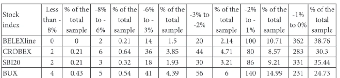
Table 3. Daily returns characteristics (left tail) of the stock indexes in the period 10.01.2006 – 31.08.2010

Stock index

Less than -8%

% of the total sample

-8% to -6%

-6% to -3%

-3% to -2%

-2% to -1%

-1% to 0%

BELEXline 0 0 2 0.21 14 1.5 20 2.14 100 10.71 362 38.76

CROBEX 2 0.21 6 0.64 36 3.85 44 4.71 80 8.57 283 30.3

SBI20 2 0.21 3 0.32 18 1.93 30 3.21 86 9.21 331 35.44

BUX 4 0.43 5 0.54 41 4.39 56 6 140 14.99 231 24.73

Source: Authors' calculations

(19)

BELEXline has a high number of days with negative returns, and most of the returns are in the intervals from -1% to 0% and from -2% to -1%.

Table 4. Daily returns characteristics (right tail) of the stock indexes in the period 10.01.2006 – 31.08.2010

Stock index 0% to 1%

2% to 3%

3% to 6%

6% to 8%

More than 8%

BELEXline 327 35.01 76 8.14 22 2.36 9 0.96 2 CROBEX 294 31.48 113 12.1 46 4.93 26 2.78 4 SBI20 328 35.12 95 10.17 29 3.1 10 1.07 2 BUX 240 25.7 114 12.21 54 5.78 45 4.82 4 Source: Authors' calculations

Compared to BELEXline, SBI20 has many less days with negative returns in the intervals from -1% to 0% and -2% to -1%. CROBEX has the greatest number of positive returns of all observed stock indexes. A large number of these returns belong to the intervals of less than -8%, from -8% to -6% and from -3% to -2%. BUX is characterized by a high number of negative returns when compared to other stocks indexed, and is so in intervals of less than -8%, from -8% to -6%, from -6% to -3%, and from -3% to -2%.

Table 5. Daily returns characteristics (left and right tail-summary) of the stock indexes in the period 10.01.2006 – 31.08.2010

Stock index -8% to 0%

0% to 8%

BELEXline 498 53.32 436 46.68

CROBEX 451 48.29 483 51.71

SBI20 470 50.32 464 49.68

BUX 477 51.07 457 48.93

(20)

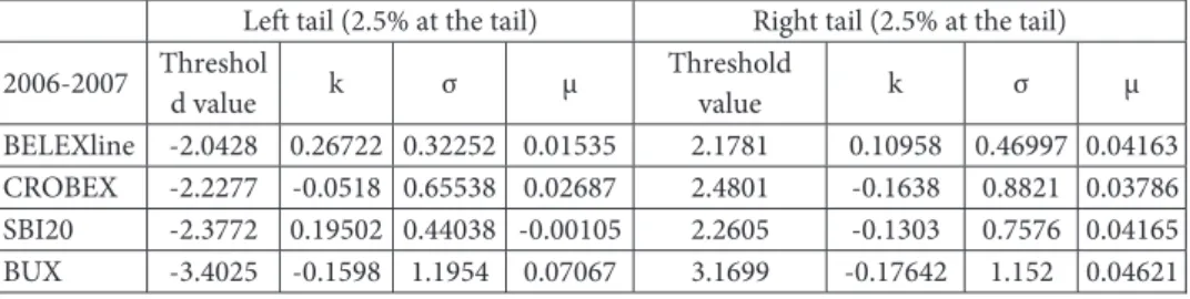
01.01.2008 – 31.08.2009) and the threshold value was obtained on the basis of the Generalized Pareto Distribution (GPD). In Table A1-1 and Table A1-2 the threshold values are shown for the in-sample period of 2006-2007. The analysis of the left tail shows that the threshold value was the least at BELEXline, SBI20, CROBEX, and BUX, respectively. The analysis of the right tail indicates that the threshold values were very alike for BELEXline and SBI20, while the same was higher at CROBEX and BUX, respectively. The reasons for these threshold value distributions lie in the distribution of daily returns and their values. Namely, BELEXline has a great number of negative returns but with less value, while SBI20 has a lower number of negative returns but with higher values (Tables 3, 4 and 5). Also, threshold values direct attention to the aforementioned characteristics of the observed stock indexes.

(21)

returns. At the left and right tails, BELEXline has the least threshold values, followed by SBI20, CROBEX, and BUX, respectively. For the left tail in 2006 and in the period 2006-2007 it was characteristic of the threshold value of CROBEX to be nearer to the threshold value of BELEXline and SBI20, while in the periods 2006-2008 and 2006-2009 the same was closer to the threshold values of the BUX. For the right tail, all threshold values are characterized by the same trend, with the exception that the threshold values of BUX are higher than in the other stock indexes. In the period 2006-2009 the threshold values did not increase at the left and the right tail, but kept their values from the previous period.

5. RESULTS AND DISCUSSION

In this section of the paper the results of the research based on GPD estimates for the BELEXline, CROBEX, SBI20, and BUX stock indexes are to be presented and analyzed. The analysis is performed for each distribution tail (2.5% and 5% at the tail) separately, to test the estimation possibilities of the maximal loss (left tail) and maximal profit (right tail) in investment activities. The research includes the performance analysis and application adequacy of two calculation approaches of GPD, i.e. the limited (two years' daily returns data) and the long interval on the selected emerging markets. The returns value in investment activities is successfully estimated in the case where the returns value of the following day is higher than the left tail estimate, but less than the right tail estimate. Otherwise the estimation was unsuccessful.

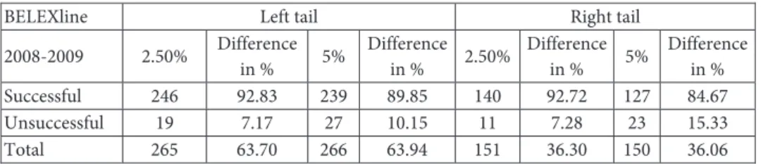
Table 6. Performance testing of the GPD application for BELEXline in the period 2008-2009 - limited interval

BELEXline Left tail Right tail

2008-2009 2.50% Difference in % 5%

Difference in % 2.50%

Difference in % 5%

Difference in % Successful 249 93.96 244 91.73 142 94.04 135 90.00 Unsuccessful 16 6.04 22 8.27 9 5.96 15 10.00 Total 265 63.70 266 63.94 151 36.30 150 36.06 Source: Authors' calculations

(22)

there are no significant differences in the percentage of success of the estimations in predicting the values of the returns by the approaches calculating the GPD, i.e. the difference is not higher than 2%. The difference in percentage is higher at the right tail (5% at the tail) and it is 5.33%. The results show that the estimate is more successful with the limited than with the long interval calculation of the GPD.

Table 7. Performance testing of GPD application for BELEXline, 2008-2009 -long interval

BELEXline Left tail Right tail

2008-2009 2.50% Difference in % 5%

Difference in % 5%

In Tables 8 and 9, the results of the application of the mentioned approaches of GPD calculation are presented for CROBEX in the period 2008-2009.

Table 8. Performance testing of the GPD application for CROBEX in the period 2008-2009 - limited interval

CROBEX Left tail Right tail

2008-2009 2.50% Difference in % 5%

Difference in % 5%

(23)

Table 9. Performance testing of the GPD application for CROBEX in the period 2008-2009 - long interval

2008-2009 2.50% Difference in % 5%

Difference in % 5%

In Tables 10 and 11, the results of the application of the mentioned approaches of GPD calculation are presented for SBI20 in the period 2008-2009.

Table 10. Performance testing of the GPD application for SBI20 in the period 2008-2009 - limited interval

SBI20 Left tail Right tail

2008-2009 2.50% Difference in % 5%

Difference in % 5%

The results of the success of the value estimations of the returns in both approaches of calculating the GPD are almost identical at SBI20. The differences are minimal both in the case of the left and the right tail, because the percentage of unsuccessful estimations are around and less than 1.5%.

Table 11. Performance testing of the GPD application for SBI20 in the period 2008-2009 - long interval

2008-2009 2.50% Difference in % 5%

Difference in % 5%

(24)

In Tables 12 and 13, the results of the application of the mentioned approaches of GPD calculation are presented for BUX in the period 2008-2009.

Table 12. Performance testing of the GPD application for SBI20 in the period 2008-2009 - limited interval

BUX Left tail Right tail

2008-2009 2.50% Difference in % 5%

Difference in % 5%

The results of the success of the value estimations of the returns in both approaches of calculating the GPD are almost identical at BUX. The differences are minimal both in the case of the left and the right tail, because the percentage of unsuccessful estimations are around and less than 2%.

Table 13. Performance testing of the GPD application for SBI20 in the period 2008-2009 - long interval

BUX Left tail Right tail

2008-2009 2.50% Difference in % 5%

Difference in % 5%

(25)

10.15% (long interval), as well as at BUX, 11.57% (limited interval) and 11.11% (long interval). The next in line is SBI20 with 12.17% (limited interval) and 13.91% (long interval); and finally CROBEX with 16.67% (limited interval) and 20.83% (long interval) of unsuccessful estimations.

The results of the research in the period 2008-2009 (Tables 6, 7, 8, 9, 10, 11, 12 and 13) for the right tail (2.5% at the tail) show that the least number of unsuccessful estimations are to be found at BELEXline, 5.96% (limited interval) and 7.28% (long interval); followed by the results at CROBEX, 6.60% (limited interval) and 8.63% (long interval). They are followed by SBI20, 8.79% (limited interval) and 8.24 % (long interval), and finally at BUX, 10.05% (limited interval) and 11.56% (long period) of unsuccessful estimations. For the right tail (5% at the tail) the least number of unsuccessful estimation results are to be found at SBI20, 10.44% (limited interval) and 10.44% (long interval); followed by BELEXline, 10.00% (limited interval) and 15.33% (long interval); CROBEX with 12.18% (limited interval) and 16.24% (long interval); and finally, BUX with 16.08% (limited interval) and 16.08% (long interval) of unsuccessful estimations.

The results of the research for 2008 (Tables A5, A6, A9, A10, A13, A14, A17 and A18) for the left tail (2.5% at the tail) show that the least number of unsuccessful estimations are to be found at BELEXline, 9.25% (limited interval) and 10.40% (long interval); followed by the results at BUX, 11.35% (limited interval) and 9.22% (long interval). They are followed by SBI20, 12.84% (limited interval) and 13.51 % (long interval), and finally at CROBEX 13.04% (limited interval) and 18.12% (long period). For the left tail (5% at the tail) the least number of unsuccessful estimation results are to be found at BELEXline, 11.05% (limited interval) and 13.37% (long interval); followed by BUX, 17.02% (limited interval) and 14.89% (long interval); SBI20 with 18.79% (limited interval) and 20.81% (long interval); and finally CROBEX, with 24.64% (limited interval) and 28.26% (long interval) of unsuccessful estimations.

(26)

and 8.11% (long interval), followed by the results at BELEXline, 8.97% (limited interval) and 8.97% (long interval). The next in line is BUX, 12.84% (limited interval) and 12.84 % (long interval), and finally at SBI20, 14.43% (limited interval) and 13.40% (long period) of unsuccessful estimations. For the right tail (5% at the tail) the least number of unsuccessful estimation results are to be found at BELEXline, 10.26% (limited interval) and 12.66% (long interval); followed by CROBEX, 12.61% (limited interval) and 14.41% (long interval); SBI20 with 15.46% (limited interval) and 15.46% (long interval); and finally BUX, with 15.60% (limited interval) and 15.60% (long interval) of unsuccessful estimations.

For all tested stock indexes in 2008, the number of days with negative returns (left tail) is considerably higher than those with positive returns (right tail). In 2008, at BELEXline the results show that the differences in successful estimations of the returns value approaches of GPD calculations are within 3% at the left tail, while the difference at the right tail is 2.5 %, and as such it can be concluded that the success is almost the same (Tables A5 and A6). At CROBEX the analysis of the results for both approaches of GDP calculation show that the differences of the successful estimation of the returns value are within 5.08% at the left tail, while the difference at the right tail is within 2%, and as such it can be concluded that the success of both approaches is almost the same (Tables A9 and A10). The analysis of the results of the differences for both approaches of GDP calculation of the successful estimation of the returns value at SBI20, show that there are no considerable differences in successfully estimates, i.e. there are no significant differences in the application of the two approaches to the investment process (Tables A13 and A14). In Tables A17 and A18, the results of the differences of the successful estimation of the returns value approaches of GPD calculation are shown at BUX in 2008. The results show that at the right tail the difference is within 2.13% (2.5% at the tail), while there are no differences of the same at 5% at the tail. In addition the results show that the estimations are more successful in the case of the long interval.

(27)

of unsuccessful estimations (limited interval) and 1.09% (long interval). The next is CROBEX with 1.28% (limited interval) and 1.28% (long interval); and finally, BUX with 1.33% (limited interval) and 1.33% (long interval) of unsuccessful estimations. For the left tail (5% at the tail) the least percentage of unsuccessful estimations is at SBI20, 0% (limited interval) and 1.23% (long interval); then BELEXline, 1.09% (limited interval) and 2.17% (long interval); BUX, 2.67% (limited interval) and 2.67% (long interval); and finally CROBEX with 2.56% (limited interval) and 7.69% (long interval) of unsuccessful estimations.

The research results in 2009 (Tables A7, A8, A11, A12, A15, A16, A19 and A20), for the right tail (2.5% at the tail) show that the least number of unsuccessful estimations is at SBI20, 2.35% (limited interval) and 2.35% (long interval), followed by BELEXline with 2.74% unsuccessful estimations (limited interval) and 5.48% (long interval). The next is CROBEX with 4.65% (limited interval) and 9.30 (long interval), and finally BUX with 6.67% (limited interval) and 10.00% (long interval) of unsuccessful estimations. For the right tail (5% at the tail) the least percentage of unsuccessful estimations is at SBI20, 4.71% (limited interval) and 4.71% (long interval); then BELEXline, 9.72% (limited interval) and 20.55% (long interval); CROBEX, 11.63% (limited interval) and 18.60% (long interval); and finally BUX with 16.67% (limited interval) and 16.67% (long interval) of unsuccessful estimations.

(28)

and A16, it can be concluded that at SBI20 the difference in the successful estimations of the returns value in GPD calculations in the investment process is 1.23%. In Tables A19 and A20 the results of the success of the GPD calculation approaches are shown for BUX for the year 2009. The results show that there are no differences in the success of the value estimations of the returns in the GPD calculations for the left tail, while for the right tail it is 3.33% (2.5% at the tail). At the right tail the number of unsuccessful estimations is less using the limited interval and is higher when the long interval of GPD calculations are used. The results show that at BELEXline, CROBEX, SBI20, and BUX the success of estimating the returns was higher at the threshold value that was calculated at the limited interval. This fact is the consequence of the volatility peculiarities of emerging markets. The volatility of these markets point to the necessity of the adequate specification of the limits in threshold calculations (optimal threshold determination), and this is especially true if the estimation successes of the returns values of the named approaches of GPD calculations are taken into consideration. The threshold value in highly volatile circumstances has to be adequate, i.e. it cannot be too high in relation to the days with less volatility (slight changes in daily returns), because this has a direct impact on the performance of the tested approaches.

(29)

BELEXline the range is 15.98% and 16.84% for the daily returns, respectively. According to these results we can conclude that the range in which the changes of returns oscillate in the period 2006-2009 is high.

6. CONCLUDING REMARKS

Risk management has undergone vast changes and gained importance in the last decade due to the increase in the volatility of financial markets, and especially due to the present world economic crisis. This paper has tested the success of the application of the extreme value theory (EVT) in estimating and forecasting the tails of daily return distribution of the analyzed stock indexes in the emerging markets of Serbia, Croatia, Slovenia, and Hungary during the 2006-2009 period. The movements of the returns of the Serbian (BELEXline), Croatian (CROBEX), Slovenian (SBI20), and Hungarian (BUX) stock indexes have been analyzed, i.e. the losses (the left tail) and profits (the right tail) of investment activity. The findings of this research show beyond any doubt the necessity of applying market risk estimation methods, i.e. extreme value theory (EVT), in the framework of a broader analysis of investment processes in emerging markets.

(30)

The daily returns' considerable oscillations influence the estimation success of the return values of the GPD calculation approaches, i.e. their success testing for the left and right tails (both 2.5% and 5% at the tail). When the GPD calculation is carried out on the limited interval the occurrence of higher daily return values moves the threshold value to the left side for the left tail, and to the right side for the right tail. Due to the shorter period of observation a small number of extremely high daily return values are enough to abruptly change the threshold value. As a consequence a shift of the threshold value occurs (following the change), and so the success of the GPD approach of estimation increases. In GPD calculations using the long interval, the in-sample days with higher daily return values do not result in a considerable change of the threshold value, because the higher number of observation points do not allow abrupt changes in the threshold value. Consequently the GPD calculation of the long interval represents a more rigorous approach, because the oscillations are less after a new day of threshold value calculations is taken into account. For this reason its success is less when compared to GPD calculations with limited interval. The threshold value has high amplitude of changes (is of higher values), especially following a period with great changes (oscillations) of returns.

When daily return oscillations decrease, the success of the GPD calculations using the limited interval is considerable because the threshold value is high, but with the remark that as a result of this on most days the threshold value to a great measure spans the values of the daily returns. Using GPD calculations with the long interval the threshold value is less, because the greater number of calculation values do not allow considerable changes in its value, and as such extreme oscillations of daily returns do not influence the threshold value very much. The threshold value in the long period is more stabile, oscillates less, and the extreme values are in a smaller range. This conditions a less successful result in estimating the values of the returns of the GPD calculation approach, because the days with extreme values of return span the threshold value, but this approach represents a more stabile measure in periods without extreme values, because the estimation is more precise and has less deviation.

(31)

success, it is necessary to view the span of the threshold value compared to daily returns. For high threshold values greater success is gained by applying the GPD approach, but in that case the threshold value is much higher than the daily return values in a stable period without high stock index value oscillations in the selected emerging markets. With high threshold values an excessive capital allocation (overestimation of the return) is necessary, which represents a loss in investment processes, and especially so when daily returns are considerably under the threshold value. In practice one hardly knows whether an applied model will under-predict or over-predict the risk in the investment process. According to the results of the research, i.e. testing the performance of the application of the extreme value theory (EVT) on the selected emerging markets, the guidelines for further research should include continuous monitoring of the success of market risk estimations (losses) and profits in investment processes, with special emphasis on the role of optimal threshold determination in increasing the success of estimating the value of returns, and especially so in conditions of global recession.

Bensalah, Y. (2000). Steps in Applying Extreme Value heory to Finance: A Review, Working Paper, Bank of Canada.

Bessis, J. (2002). Risk Management in Banking, 2nd_{edition, New York: John Wiley & Sons.}

Coronel-Brizio, H.F. & Hernandez-Montoya, A.R. (2005). On itting the Pareto–Levy distribution to stock market index data: Selecting a suitable cutof value, Physica A., Vol. 354, pp. 437-449. Dacorogna, M.M. et al. (2001). An Introduction to High Frequency Finance, San Diego: Academic

Press.

Da Silva, L.C.A. & de Melo Mendez, B.V. (2003). Value-at-Risk and Extreme Returns in Asian Stock Markets, International Journal of Business, Vol. 8, No. 1, pp. 17-40.

Danielsson, J. & C.G. de Vries (1997). Value at Risk and Extreme Returns, FMG Discussion paper No. 273, Financial Markets Group, London School of Economics.

(32)

Danielsson, J. & C.G. de Vries (2002). Where do Extremes Matter? Working Paper, http://www. RiskResearch.org

Dowd, K. (1998). Beyond Value at Risk: he New Science of Risk Management, Chichester: John Wiley & Sons.

Drenovak, M. & Urosevic, B. (2010). Modelling the benchmark spot curve for the Serbian market,

Economic Annals, Vol. 55, No. 184, pp. 29-57.

Duie, D., & J. Pan (1997). An overview of Value-at-Risk, Journal of Derivates, Vol. 7, pp. 7-49. Embrechts, P., Klüppelberg, C. & Mikosch, T. (1997). Modeling Extremal Events for Insurance and

Finance, New York: Springer.

Embrechts, P., Resnick, S. & Samorodnitsky, G. (1999). Extreme Value heory as a Risk Management Tool, North American Actuarial Journal, Vol. 3, No. 2, pp. 30-41.

Gencay, R. & Selcuk, F. (2004). Extreme value theory and Value-at-Risk: Relative performance in emerging markets, International Journal of Forecasting, Vol. 20, pp. 287-303.

Harmantzis, F., ChienY. & Miao, L. (2005). Empirical Study of Value-at-Risk and Expected Shortfall as a Coherent Measure of Risk, Journal of Risk Finance, Vol. 7, No. 2, pp. 117-135. Hauksson, H.A. et al. (2000). Multivariate extremes, aggregation and risk estimation, Manuscript,

Ithaca, NY: School of Operations Research and Industrial Engineering, Cornell University.

Jorion, P. (1996). Value at Risk: he New Benchmark for Controlling Market Risk, Chicago: Irwin. Jorion, P. (2001). Value at Risk: he New Benchmark for Managing Financial Risk, 2nd edition,

New York: McGraw Hill.

Linsmeier, T.J. & Pearson, N.D. (2000). Value at Risk, Financial Analysts Journal, Vol. 56, No. 2, pp. 47-67.

Marinelli, C., d’Addona, S. & Rachev, S.T.(2007). A Comparison of Some Univariate Models for Value-at-Risk and Expected Shortfall, International Journal of heoretical and Applied Finance, Vol. 10, No. 6, pp. 1-33.

McNeil, A.J. (1997). Estimating the Tails of Loss Severity Distribution Using Extreme Value heory, heory ASTIN Bulletin, Vol. 27, No. 1, pp. 1117-1137.

(33)

Mladenovic, Z. and Mladenovic, P. (2006). Estimation of the value-at-risk parameter: econometric analysis and the extreme value theory approach, Economic Annals, Vol. 51, No. 171, pp. 32-73. Nuti, M.D. (2009). he impact of the global crisis on transition economies, Economic Annals, Vol.

54, No. 181, pp. 7-20.

Obadovic, M.D. & Obadovic, M.M. (2009). An analytical method of estimating Value-at-Risk on the Belgrade Stock Exchange, Economic Annals, Vol. 54, No. 183, pp. 119-138.

Salomons, R. & Grootveld, H. (2003). he equity risk premium: emerging vs. developed markets,

Emerging Markets Review, Vol. 4, Issue 2, pp. 121-44.

Seymour, A. J. & Polakow, D.A. (2003). Coupling of Extreme-Value heory and Volatility Updating with Value-at-Risk Estimation in Emerging Markets: A South African Test, Multinational Finance Journal, Vol. 7, No. 1&2, pp. 3-23.

(34)

APPENDIX

Table A1-1. Threshold value for the in-sample period 2006-2007 (2.5% at the tail)

Left tail (2.5% at the tail) Right tail (2.5% at the tail)

2006-2007 Threshol

d value k σ μ

Threshold

value k σ μ

BELEXline -2.0428 0.26722 0.32252 0.01535 2.1781 0.10958 0.46997 0.04163 CROBEX -2.2277 -0.0518 0.65538 0.02687 2.4801 -0.1638 0.8821 0.03786 SBI20 -2.3772 0.19502 0.44038 -0.00105 2.2605 -0.1303 0.7576 0.04165

BUX -3.4025 -0.1598 1.1954 0.07067 3.1699 -0.17642 1.152 0.04621

Table A1-2. Threshold value for the in-sample period 2006-2007 (5% at the tail)

Left tail (5% at the tail) Right tail (5% at the tail)

2006-2007 Threshold

value k σ μ

Threshold

value k σ μ

BELEX line -1.4959 0.26722 0.32252 0.01535 1.7081 0.10958 0.46997 0.04163 CROBEX -1.8456 -0.0518 0.65538 0.02687 2.1263 -0.1638 0.8821 0.03786 SBI20 -1.791 0.19502 0.44038 -0.00105 1.9207 -0.1303 0.7576 0.04165

BUX -2.9165 -0.1598 1.1954 0.07067 2.7268 -0.17642 1.152 0.04621

Table A2-1. Threshold value – limited interval (2.5% at the tail)

Observation

period Stock index

Threshold

value k σ μ

Threshold

value k σ μ

2006-2007 BELEXline -2.042 0.26722 0.32252 0.01535 2.178 0.10958 0.46997 0.04163

2007-2008 BELEXline -3.815 0.16183 0.74886 0.03656 3.759 0.20716 0.67893 -9.37E-04

2008-2009 BELEXline -3.739 -0.00517 0.99776 0.09398 4.537 -0.045 1.3591 -0.08168

2006-2007 CROBEX -2.227 -0.05175 0.65538 0.02687 2.48 -0.1638 0.8821 0.03786

2007-2008 CROBEX -6.218 0.16494 1.228 -0.0178 4.578 0.1627 0.89228 0.06759

2008-2009 CROBEX -6.865 -0.02698 1.9588 -0.01266 6.075 0.04802 1.5022 0.01288

2006-2007 SBI20 -2.377 0.19502 0.44038 -0.00105 2.26 -0.1303 0.7576 0.04165

2007-2008 SBI20 -5.205 0.11832 1.1149 0.04917 3.797 0.06535 0.88983 0.08568

2008-2009 SBI20 -5.181 0.13544 1.0574 0.2117 4.341 0.07601 1.0086 0.04646

2006-2007 BUX -3.402 -0.15979 1.1954 0.07067 3.169 -0.17642 1.152 0.04621

2007-2008 BUX -5.746 0.17435 1.082 0.14574 5.225 0.21571 0.91203 0.08354

2008-2009 BUX -6.563 -0.00931 1.7755 0.1254 6.971 -0.00602 1.9094 0.00504

(35)

Table A2-2. Threshold value – limited interval (5% at the tail)

Left tail (5% at the tail) Right tail (5% at the tail) Observation

period Stock index

Threshold

value k σ μ

Threshold

value k σ μ

2006-2007 BELEXline -1.4959 0.26722 0.32252 0.01535 1.708 0.10958 0.46997 0.04163

2007-2008 BELEXline -2.9234 0.16183 0.74886 0.03656 2.817 0.20716 0.67893 -9.37E-04

2008-2009 BELEXline -3.06 -0.0052 0.99776 0.09398 3.727 -0.045 1.3591 -0.08168

2006-2007 CROBEX -1.8456 -0.0518 0.65538 0.02687 2.126 -0.1638 0.8821 0.03786

2007-2008 CROBEX -4.74 0.16494 1.228 -0.0178 3.512 0.1627 0.89228 0.06759

2008-2009 CROBEX -5.6245 -0.027 1.9588 -0.01266 4.852 0.04802 1.5022 0.01288

2006-2007 SBI20 -1.791 0.19502 0.44038 -0.00105 1.92 -0.1303 0.7576 0.04165

2007-2008 SBI20 -4.0576 0.11832 1.1149 0.04917 3.03 0.06535 0.88983 0.08568

2008-2009 SBI20 -4.0285 0.13544 1.0574 0.2117 3.439 0.07601 1.0086 0.04646

2006-2007 BUX -2.9165 -0.1598 1.1954 0.07067 2.726 -0.17642 1.152 0.04621

2007-2008 BUX -4.4024 0.17435 1.082 0.14574 3.923 0.21571 0.91203 0.08354

2008-2009 BUX -5.3708 -0.0093 1.7755 0.1254 5.673 -0.00602 1.9094 0.00504

Table A3-1. Threshold value – long interval (2.5% at the tail)

Stock index Observation

period

Threshold

value k σ μ

Threshold

value k σ μ

BELEXline 2006 -0.875 -0.1096 0.28794 0.00185 1.007 -0.39508 0.50691 0.02295

2006-2007 -2.042 0.26722 0.32252 0.01535 2.178 0.10958 0.46997 0.04163

2006-2008 -3.38 0.23651 0.57231 0.01017 2.923 0.24982 0.47764 0.03002

2006-2009 -3.297 0.12302 0.70525 0.00489 3.383 0.17726 0.64871 0.0059

CROBEX 2006 -1.644 -0.2112 0.63394 0.02039 2.202 -0.18916 0.82451 0.01287

2006-2007 -2.227 -0.0518 0.65538 0.02687 2.48 -0.1638 0.8821 0.03786

2006-2008 -5.346 0.24863 0.88311 0.01089 3.835 0.12008 0.81353 0.05411

2006-2009 -5.57 0.18841 1.0449 0.00422 4.376 0.10414 0.96318 0.04492

SBI20 2006 -1.333 0.15905 0.26379 0.01004 1.846 -0.01002 0.4990.3 0.03941

2006-2007 -2.377 0.19502 0.44038 -0.00105 2.26 -0.1303 0.7576 0.04165

2006-2008 -4.536 0.23062 0.78265 -0.01555 3.303 0.09597 0.73415 0.05401

2006-2009 -4.182 0.18929 0.78247 0.00622 3.225 0.04545 0.79027 0.05116

BUX 2006 -3.78 -0.2216 1.4978 0.00587 3.404 -0.26676 1.4239 0.06156

2006-2007 -3.402 -0.1598 1.1954 0.07067 3.169 -0.17642 1.152 0.04621

2006-2008 -5.168 0.08611 1.1646 0.11151 4.639 0.0934 1.0343 0.0843

2006-2009 -5.243 0.00485 1.3839 0.09262 5.31 0.06294 1.2655 0.05539

(36)

Table A3-2. Threshold value – long interval (5% at the tail)

Left tail (5% at the tail) Right tail (5% at the tail) Stock index Observation

period

Threshold

value k σ μ

Threshold

value k σ μ

BELEXline 2006 -0.737 -0.1096 0.28794 0.00185 0.913 -0.39508 0.50691 0.02295

2006-2007 -1.495 0.26722 0.32252 0.01535 1.708 0.10958 0.46997 0.04163

2006-2008 -2.505 0.23651 0.57231 0.01017 2.159 0.24982 0.47764 0.03002

2006-2009 -2.559 0.12302 0.70525 0.00489 2.57 0.17726 0.64871 0.0059

CROBEX 2006 -1.427 -0.2112 0.63394 0.02039 1.898 -0.18916 0.82451 0.01287

2006-2007 -1.845 -0.0518 0.65538 0.02687 2.126 -0.1638 0.8821 0.03786

2006-2008 -3.939 0.24863 0.88311 0.01089 2.991 0.12008 0.81353 0.05411

2006-2009 -4.21 0.18841 1.0449 0.00422 3.431 0.10414 0.96318 0.04492

SBI20 2006 -1.022 0.15905 0.26379 0.01004 1.512 -0.01002 0.4990.3 0.03941

2006-2007 -1.791 0.19502 0.44038 -0.00105 1.92 -0.1303 0.7576 0.04165

2006-2008 -3.362 0.23062 0.78265 -0.01555 2.602 0.09597 0.73415 0.05401

2006-2009 -3.16 0.18929 0.78247 0.00622 2.587 0.04545 0.79027 0.05116

BUX 2006 -3.284 -0.2216 1.4978 0.00587 2.998 -0.26676 1.4239 0.06156

2006-2007 -2.916 -0.1598 1.1954 0.07067 2.726 -0.17642 1.152 0.04621

2006-2008 -4.091 0.08611 1.1646 0.11151 3.659 0.0934 1.0343 0.0843

2006-2009 -4.268 0.00485 1.3839 0.09262 4.227 0.06294 1.2655 0.05539

Table A4-1. Threshold value for the left tail for each tested index (2.5% at the tail)

Stock index Left tail 2006-2007 2006-2008 2006-2009

BELEXline Limited interval -2.042 -3.815 -3.739

Long interval -2.042 -3.38 -3.297

CROBEX Limited interval -2.227 -6.218 -6.865

Long interval -2.227 -5.346 -5.570

SBI20 Limited interval -2.377 -5.205 -5.181

Long interval -2.377 -4.536 -4.182

BUX Limited interval -3.402 -5.746 -6.563

Long interval -3.402 -5.168 -5.243

(37)

Table A4-2. Threshold value for the left tail for each tested stock index (5% at the tail)

Stock index Left tail 2006-2007 2006-2008 2006-2009

BELEXline Limited interval -1.4959 -2.9234 -3.06 Long interval -1.4959 -2.505 -2.5595

CROBEX Limited interval 1.8456 -4.74 -5.6245 Long interval -1.8456 -3.9396 -4.2104

SBI20 Limited interval -1.791 -4.0576 -4.0285 Long interval -1.791 -3.3627 -3.1606

BUX Limited interval -2.9165 -4.4024 -5.3708 Long interval -2.9165 -4.0917 -4.2687 Source: Authors' calculations

Table A4-3. Threshold value for the right tail for each tested stock index (2.5% at the tail)

Stock index Right tail 2006-2007 2006-2008 2006-2009

BELEXline Limited interval 2.178 3.759 4.537

Long interval 2.178 2.923 3.383

CROBEX Limited interval 2.48 4.578 6.075 Long interval 2.48 3.835 4.376

SBI20 Limited interval 2.26 3.797 4.341 Long interval 2.26 3.303 3.225

BUX Limited interval 3.169 5.225 6.971

Long interval 3.169 4.639 5.31 Source: Authors' calculations

Table A4-4. Threshold value for the right tail for each tested stock index (5% at the tail)

Stock index Right tail 2006-2007 2006-2008 2006-2009

BELEXline Limited interval 1.7081 2.8177 3.7273 Long interval 1.7081 2.15952 2.5701

CROBEX Limited interval 2.1263 3.5125 4.8529 Long interval 2.1263 2.991 3.4311

SBI20 Limited interval 1.9207 3.0302 3.4396 Long interval 1.9207 2.6021 2.5873

BUX Limited interval 2.7268 3.9238 5.6738

(38)

Table A5. Performance testing of the GPD application for BELEXline in 2008 – limited interval

BELEX line Left tail Right tail

2008 2.50% Difference in % 5%

Difference in % 5%

Table A6. Performance testing of the GPD application for BELEXline in 2008 – long interval

Difference in % 5%

Table A7. Performance testing of the GPD application for BELEXline in 2009 – limited interval

Difference in % 5%

(39)

Table A8. Performance testing of the GPD application for BELEXline in 2009 – long interval

Difference

in % 2.50%

Difference in % 5%

Table A9. Performance testing of the GPD application for CROBEX in 2008 – limited interval

Difference in % 5%

Table A10. Performance testing of the GPD application for CROBEX in 2008 – long interval

Difference in % 5%

(40)

Table A11. Performance testing of the GPD application for CROBEX in 2009 – limited interval

Difference in % 5%

Difference in % Successful 77 98.72 76 97.44 82 95.35 76 88.37 Unsuccessful 1 1.28 2 2.56 4 4.65 10 11.63 Total 78 47.56 78 47.56 86 52.44 86 52.44

Table A12. Performance testing of the GPD application for CROBEX in 2009 – long interval

Difference in % 5%

Table A13. Performance testing of the GPD application for SBI20 in 2008 – limited interval

Difference in % 5%

(41)

Table A14. Performance testing of the GPD application for SBI20 in 2008 – long interval

Difference in % 5%

Table A15. Performance testing of the GPD application for SBI20 in 2009 – limited interval

Difference in % 5%

Table A16. Performance testing of the GPD application for SBI20 in 2009 – long interval

Difference in % 5%