From public to private: the performance of former public workers in the Brazilian labor market

From Public to Private:

The Performance of Former Public Workers in the Brazilian Labor Market∗

Sergio Firpo

Department of Economics, UC Berkeley

Gustavo Gonzaga

Department of Economics, PUC-Rio

Preliminary Version – June 2002

Abstract

This paper analyzes the placement in the private sector of a subset of Brazilian public-sector employees. This group left public employment in the mid-1990’s through a voluntary severance program. This paper contrasts their earnings before and after quitting the public sector, and compares both sets of wages to public and private sector earnings for similar workers. We find that participants in this voluntary severance program suffered a significant reduction in average earnings wage and an increase in earnings dispersion. We test whether the reduction in average earnings and the increase in earnings dispersion is the expected outcome once one controls for observed characteristics, by means of counterfactual simulations. Several methods of controlling for observed characteristics (parametric and non-parametrically) are used for robustness. The results indicate that this group of workers was paid at levels below what would be expected given their embodied observable characteristics.

JEL Code: J45

Keywords: Public Sector Downsizing, Public-Private Wage Gap, Earnings Inequality

I. Introduction

Mainly forced by a chronic public deficit problem, the Brazilian federal government exerted substantial efforts to reduce the number of public servants in the second half of the 1990’s. In some cases, the government was concerned with the social welfare impact of such major layoffs. In fact, the design of an efficient public sector downsizing program depends heavily on an estimation of the

capacity of the private sector to absorb former public workers.1

Given the existing legal constraints on firing public workers and an overall opposition to public sector reform in Brazil, the federal government typically opted for voluntary job retrenchment schemes. Many state firms, in a step towards privatization, promoted the so-called

Voluntary Severance Programs (Programas de Demissão Voluntária, PDV), which gave monetary

incentives to workers who quit their jobs.2 In a developing country like Brazil, characterized by

overstaffing, it is expected that PDV´s result in an adverse selection outcome, with the best workers, those with higher reservation wages, opting to leave. On the other hand, the fact that these workers usually have very specific human capital, combined with a possible stigma effect, can reduce both the probability of absorption and expected earnings in the private sector.

In 1995, Rede Ferroviária Federal S.A. (RFFSA), a huge public firm that had the

monopoly on all Brazilian railways, adopted a PDV. From 1995 to the end of 1997 more than 7,000 workers joined the program, while many others opted for early retirement. A first survey with those

former employees at RFFSA was conducted in March 1998.3 It revealed that their reinsertion in the

private labor market was not a success, although many workers were absorbed by the private sector.

Figure 1 below is the main motivation for this paper. It gives a striking picture of the performance of these former public workers, by summarizing the distributions of real earnings of previous RFFSA workers before and after leaving the firm. The picture shows that average real earnings dropped by 15,4%, while earnings inequality dramatically increased. In fact, 72% of these

workers observed reductions in real earnings.4 A significant proportion (31%) of these workers

were receiving less than R$300,00 (2,5 times the minimum wage) in the private sector in 1997. This contrasts with a very small proportion (0,16%) of these workers that were in this earnings range in 1995, while at RFFSA.

These results are in a certain way expected. It is a well-documented fact that Brazilian

public employees earn on average more than workers at the private sector (see Foguel et al., 2000).

On the other hand, a comparison between public and private sectors in Brazil and other Latin American countries reveals that wage inequality among workers in the private sector is typically significantly higher than among public employees (see Panizza and Qiang, 2000). Therefore, it is also not surprising that the earnings distribution widened among these former public employees. The interesting comparison, however, is with the expected earnings distributions of these workers in the private sector, given their observable characteristics.

1

See Rama (1999) for a survey of several studies on public sector downsizing.

2

In fact, PDV’s were also applied at the federal administrative level and by many states, targeting a variety of workers and locations. Particular emphasis, however, was given to state enterprises, since the government had a special interest in privatizing some of these firms and needed a fast payroll reduction. See Carneiro and Gill (1999) for a description of public sector downsizing programs in Brazil.

3 _{The details of that survey are described in Section II and more fully in Amadeo, Camargo and Gonzaga (1998).} 4

Figure 1

Log-earnings density function - REDE Employees: before and after leaving public sector

0 0,2 0,4 0,6 0,8 1 1,2

0 2 4 6 8 10

log-earnings (real terms)

12

Before After R$100 (97) R$120 (97 - Min Wage)

The main objective of this paper is to compare the outcomes of the former RFFSA employees with those in the public and private sectors in Brazil. We investigate how have these workers performed in the private sector, once we take into consideration their observable attributes. Have they converged to a similar earnings distribution prevailing in that sector, given their observable characteristics? In order to study the process of absorption by the private sector of these workers, we use the RFFSA survey data set, in combination with information from national household surveys. Our decomposition analysis attempts to identify the role of observable characteristics, as well as their remuneration in the public and the private sector, in explaining the observed changes in the earning distributions of the former RFFSA employees. In order to deal with selection bias, we control for observable characteristics, using parametric, semi-parametric and non-parametric methods. The idea is to test how robust are the results with respect to the choice of matching techniques.

The paper is organized as follows. The next section describes the data. Section III presents the gross earnings gaps observed for the distributions used in the paper. Section IV discusses the research methodology. Section V presents and interprets the empirical results. Section VI concludes.

II. Data description

9-10, 11, 12-14, 15, and more than 15.5 REDE also contains official administrative information for all workers who joined the PDV, including their last wages at RFFSA.

The other data set, Pesquisa Nacional de Amostra por Domicílio (PNAD), is the annual

Brazilian Household Survey, collected by IBGE. PNAD covers the whole country, with the exception of some rural areas. It is the largest and most important Brazilian household survey, interviewing more than 75,000 households every year, which corresponds to about 300,000 individuals. PNAD collects data every September since 1976, with the exception of Census years and a couple of other years. It contains information on labor, demographic, educational and regional variables and has been widely used in many micro-econometric studies.

In this study, we use information from both data sets for men in the age range of 25-64 and

with a paid main activity that requires at least 20 weekly hours of work.6 Two yearly editions of

PNAD were selected, 1995 and 1997. These two years were chosen in order to approximately match both the timing of exit from RFFSA and the absorption of these workers by the private sector, as captured by the REDE survey.

Data on earnings correspond to positive monthly labor earnings on the main activity. This variable was properly deflated and evaluated at March 1998, the date of the REDE survey. In the PNAD data set, outliers (earnings larger than R$ 250,000 a month) are not considered in the analysis. In the REDE data set, we only use information about workers who switched to the private sector after quitting, as answered in the survey of March 1998.

Since REDE is restricted to some Federation States, only observations in the same geographical range are used in PNAD. In practice, this means that the North Region and some States in the Mid-West are not considered here. We also exclude data from rural areas and for workers in agricultural activities. Finally, the classification at PNAD for a job at the public sector has the broadest sense, meaning that not only federal public servants are considered as working in the public sector but also any individual who declared to work at that sector with or without a formal labor contract.

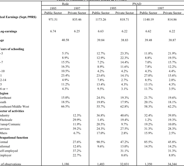
Table 1 displays summary statistics for the most important variables in the two data sets and

the number of observations remaining after the application of the filters described above.7 Note that

Rede workers are, on average, older, more educated and more concentrated in the Southeast region of the country than public and private workers (see also Figures 2a to 2d).

III. Total Earnings Gap

In this section, we analyze the average total earnings gap for the RFFSA workers that were absorbed by the private sector and decompose it into several parts. As described in the previous

section, we have information on real earnings, yi,t,s,p, for each individual i, at time t (1995 and

1997), at sector s (public and private), and for both available data sets p (REDE and PNAD).

Considering the transformation to log-earnings, wi,t,s,p = log(yi,t,s,p), we have six distributions of

log-earnings that can be used, since for REDE individuals we only have two possibilities: one was either in the private sector in 1997 or in the public sector in 1995. To fix notation, let us say that an

individual i is in market m when he faces a triple (t,s,p).

5

In fact, there are ten categories but the first two (illiteracy and less than four years of schooling) were merged into one group here. The categories corresponding to isolated years (4, 8, 11 and 15) reflect the attainment of some school degree in Brazil (elementary, medium, high school and college, respectively).

6 _{We restricted our attention to male workers since more than 91% of those former workers who entered the private}

sector are men.

7

In this paper, the main interest is in the difference between some parameters of two distributions in particular: workers that we observe in 1997 at the private sector using REDE data set and workers that we observe in 1995 at the public sector using REDE data set. For the particular

case of those two distributions, let us say that a worker is in the labor market m = 1 if we observe

him in the former distribution (1997, private, REDE) and that he is in the labor market m = 0 if we

observe him in the latter (1995, public, REDE). It turns out that because of panel features of REDE data set, those workers are the same in both distributions.

The gross total earnings gap is given by E[w1] – E[w0]. Many additional insights can be

brought by using a third distribution, w2, and noting that the difference in means, E[w1] – E[w0],

can be decomposed into the sum of two differences (E[w1] – E[w2]) + (E[w2] – E[w0]). This

decomposition in differences method allows one to split the differences in parameters of two specific distributions into several distinct partial effects.

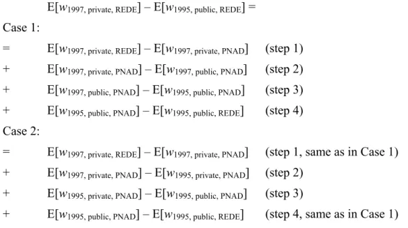
It is possible to decompose the difference between the distributions (1997, private, REDE) and (1995, public, REDE) into 4 intermediate differences. For example, one could compare the earnings distribution of former RFFSA employees with the earnings distribution of all private sector workers in 1997; then examine how the private sector earnings distribution evolved between 1995 and 1997; and finally compare the distributions of the public and the private sectors in 1995. In fact, there are two ways of decomposing the total earnings gap into 4 intermediate differences, which are described below:

E[w1997, private, REDE] – E[w1995, public, REDE] =

Case 1:

= E[w1997, private, REDE] – E[w1997, private, PNAD] (step 1)

+ E[w1997, private, PNAD] – E[w1997, public, PNAD] (step 2)

+ E[w1997, public, PNAD] – E[w1995, public, PNAD] (step 3)

+ E[w1995, public, PNAD] – E[w1995, public, REDE] (step 4)

Case 2:

= E[w1997, private, REDE] – E[w1997, private, PNAD] (step 1, same as in Case 1)

+ E[w1997, private, PNAD] – E[w1995, private, PNAD] (step 2)

+ E[w1995, private, PNAD] – E[w1995, public, PNAD] (step 3)

+ E[w1995, public, PNAD] – E[w1995, public, REDE] (step 4, same as in Case 1)

The difference between cases 1 and 2 is in steps 2 and 3. In case 1, step 3 measures the evolution of public sector earnings between 1995 and 1997, while step 2 compares the private and the public sector in 1997. In case 2, step 3 measures the difference between the public and the private sector in 1995, while step 2 captures the temporal evolution of private sector earnings.

Table 2 summarizes the results of these mean decompositions for all steps in case 1.8

8

IV. Research Methodology

In this section, we describe our methodological approach discussing several ways to estimate controlled wage gaps and the assumptions needed for consistency for each estimator in consideration.

IV.1 The controlled earnings gap and the average treatment effect

Our goal is to estimate the average difference in payments between two workers with the

same attributes but that are in different labor markets, m = 1 and m = 0. In order to do that, we use

some techniques from the traditional literature on wage gap and some others from the treatment effects literature. Note however that in this paper it is not clear what should be called the “treatment group” and what should be called the “control group”, since we are not in fact comparing treatment and control groups in an experiment.

We arbitrarily fix that a worker is in the treatment group if he belongs to the distribution m

= 1; by analogy, a worker is said to be in the control group if he belongs to the distribution m = 0.

This way we can interpret the controlled earnings differential estimations, which are comparisons

between the earnings of the average individual in m = 1 and his counterfactual earnings in m = 0, as

a “treatment effect”.9

Assuming that there are only two possible labor markets, m = 0 and m = 1, let us then

define Ti as an indicator variable such that, Ti = {individual i is at sector m = 1}. The worker i’s

observed log-wage is then:10

(1) wi = (wi,1 – wi,0) Ti + wi,0.

Following Heckman (1990), we are interested in estimating the gain from moving an m = 1

worker with a vector in Rk of observable attributes xi from sector m = 0 to m = 1. This is the

controlled earnings gap specified in a broad sense. It can be seen below that it has the same

mathematical expression of the so-called average treatment effect on the treated, which is:

(2) ∆ = Ex[∆(x)] = Ex[E[w1 | T = 1, x] – E[w0 | T = 1, x]]

The main problem of estimating ∆ in (2) is that we can never observe E[w0|T=1,x]. So,

following the literature on treatment effects, we need a slightly weaker version of the traditional

“unconfounded treatment assignment” given a set of covariates assumption (Rubin, 1977)).11 That

is, we may assume that:

(3) w_i,1,w_i,0 ⊥T_i |x_i,∀i,

9

“Treatment effect” might be a misleading term since it is not our goal to find any causal effect. However, we keep this terminology, mainly because most of the estimation procedures presented here are typical of the literature on the treatment effect.

10

For a causal interpretation, wi,1 and wi,0 should be interpreted, following the treatment effect literature, as potential

earnings of worker i in m = 1 and m = 0, respectively.

11

which implies:

(3a) E[w0|T = 1, x] – E[w0|T = 0, x] = 0.

Equation (3) states that given xi, treatment is uncorrelated to earnings. This is a strong

assumption that basically rules out any explanatory role of unobservable characteristics. With that assumption on, we might rewrite (2) as:

(4) ∆ = Ex[E[w1|T = 1, x] – E[w0|T = 1, x]] =

= Ex[E[w1|T = 1, x] – E[w0|T = 0, x]] +

+ Ex[E[w0|T = 0, x] – E[w0|T = 1, x]] =

(4a) ∆ = Ex[E[w1|T = 1, x] – E[w0|T=0, x]]

Thus, if we have discrete observable characteristics x, ∆ turns out to be:

(4b) ∆ =

∑

{

}

= = − = k J J j j j j k

j x w|T , w|T ,

x ... 1 0 1 , , 1 1 ] 0 E[ ] 1 E[ ) ,..., (

f x x

where f(.) is the probability mass function of x, a random vector that can be decomposed into J1…

Jk categories. However, if x is continuously distributed with distribution function F(.):

(4c) ∆ =

∫

{

}

Notice that it can be hard to estimate ∆(x) for every x, mainly because x is multidimensional

and might be continuously distributed. Thus, in order to estimate ∆ we need some device that

allows us to overcome such multidimensionality problem. Following Rosenbaum and Rubin

(1983), we define the propensity-score (p-score) as the probability of being in m = 1 given a set of

vector of covariates x.12 Write the propensity-score as being:

(5) p(xi) = Pr[Ti = 1| xi]

If we assume that 0 < p(xi) <1 for all workers i, it can be shown that equation (3) implies:

12

(6) w_i,1,w_i,0 ⊥T_i | p(x_i),∀i

Equation (6) reduces the problem of dimensionality to a single univariate scale, the range of

p(x). Now, note that if we know p(xi), we can proceed in an analogous way to the derivation of

equation (4a), in order to re-express ∆ as:

(7) ∆ = Ex[E[w1|T = 1, p(x)] – E[w0|T=0, p(x)]] =

(7a) ∆ = Ep(X)[E[w1|T = 1, p(x)] – E[w0|T=0, p(x)]] =

Now, let us try to reconcile this approach with the usual approach of using Mincer equations in the estimation of the controlled wage gap. A typical generalized Mincer equation is of the form:

(8) wi,j = hj(xi,j) + uj(zi,j), i = 1,…,N and j = 0,1

where z is a vector of non-observable characteristics and h(.) and u(.) are unknown real-valued

functions. We also assume that for all i:

(9) wi,j = hj(xi,j) + εi,j ;and E[wj|xj] = hj(xj), j = 0,1

i.e., that the unobservable and observable characteristics are not correlated.13

We can now, using (9), write the parameter of interest ∆ as:

(10) ∆ = Ex[∆(x)] = Ex[E[h1(x1) | T = 1, x] – E[h0(x0) | T = 1, x]]

Equation (10) can be simplified once we assume a parametric and known form for h(.):

(11) hj(xi,j) = αj + βj’xi,j, j = 0,1,

and also assuming, as in Heckman (1990), the following simplifying assumption (12), which allows us to estimate wage differentials without the need to look for complicated sample selection-correction models:

(12) E[ε1 – ε0 | T = 1, x] = 0, yielding:

13

(13) ∆ = α1 – α0 + β1’E[x1| T = 1] – β0’E[x0| T = 1] =

= α1 – α0 + (β1 – β0)’E[x1| T = 1] + β0’(E[x1| T = 1] – E[x0| T = 1]).

Now, if x1 and x0 are identically distributed, then the “composition effect” is zero, that is:

(14) β0’(E[x1| T = 1] – E[x0| T = 1]) = 0.

Finally:

(15) ∆ = α1 – α0 + (β1 – β0)’E[x| T = 1].

If we rely on an even stronger assumption on the functional forms of h1(.) and h0(.), that is,

if β1 = β0, then:

(16) ∆ = α1 – α0

IV.2 Estimation

Several approaches for estimation of ∆ were proposed in the literature. We shall present

some of them, divided into three major classes: non-parametric, semi-parametric, and parametric estimators.

IV.2.1 Non-parametric approach

The following estimator does not need any assumption on the functional form of w for its

consistency to ∆. Because of that characteristic, we call it a non-parametric estimator.14 In fact, it is

a special case of a larger class of matching estimators, as described in Heckman, Ichimura and Todd (1998).

For the case of discrete covariates, the following equation describes such estimator:

(17) ∆ˆ_np =

∑

∑

∑

∑

∑

∑∑

∑

k i k i j i i T w T T w T T T ... 1 1 1 ) 1 ( ) 1 ( 14

where the subscript np stands for non-parametric and. Notice that for such estimator to be

consistent for ∆ it suffices that the “unconfoundness assumption” (equation (3)) holds.

IV.2.2 Semi-parametric approaches15

In many situations a multidimensional vector of continuous covariates might force the use of the propensity score as described earlier. The main assumption needed for consistency of estimators based on the p-score is equation (6).

For estimators based on the p-score, a first and parametric estimation step is often made necessary: the estimation of the p-score. A traditional way of estimating the propensity score is by logistic regressions as in the equation below:

(18) Pr[Ti=1| xi] = exp(γ + δ’λ(xi))/[1 + exp(γ + δ’λ(xi))], i = 1,...,N

where λ(.) is a polynomial function to be chosen.

The fitted values of this estimation by maximum likelihood yield the estimated propensity

score, . pˆ(x_i)

IV.2.2.1 Stratifying using the Propensity Score

Now assume that our specification for the logit is enough to fully condition on the observables that make up the assignment mechanism. If that condition is satisfied then, following Rosenbaum and Rubin (1984), who proposed using a discrete distribution of the p-score to estimate

equation (7a). For that to be a feasible procedure, they use instead of p(x) to estimate ∆.

Rosenbaum and Rubin (1984) stratify the observations along quantiles of and estimate the

difference between treatment and control outcomes for each stratum. In order to check balance of covariates within each stratum, they perform F-tests to the difference in means of each covariate between treatment and control groups. They conclude that sub-classifying the sample accordingly to five quantiles of the estimated p-score yielded the desired balance.

) ( ˆ x p ) ( ˆ x p

After deciding how many strata (quantiles of ) the sample will be divided into, one

can estimate ∆ by:

) (

ˆ x

p

(19)

∑

∑

∑

∑

∑

∑∑

∑

k i k i q i i sps T w T T w T T T 1 1 ) 1 ( ) 1 ( ˆ

15 _{We are using the term semi-parametric estimation in a slightly different way from that one, for instance, that Powell}

where the subscript sps stands for “stratified on p-score”, q is a quantile of and Q is the number of quantiles that provide a good balance on the covariates.

) (

ˆ x

p

16

In this paper we use the above-mentioned estimator stratifying each pair of distributions into 50 blocks. However, as we will see in the results, even such large number of data divisions is not able to provide a good balance for some pairs.

IV.2.2.2 Reweighing using the Propensity Score

The propensity-score approach can be used to estimate ∆ in several different ways. The

previous way, stratifying on the p-score, can be seen as a special case of a matching estimator as defined by Heckman, Ichimura and Todd (1998), with weights coming from an approximate

discrete distribution of p(x). Note that although being a matching estimator in a general sense, it is

not what the literature calls “matching on the p-score”, which is well described by Angrist and Krueger (1999) and Dehejia and Wahba (1999).

Another “matching estimator” in the broad sense is the so-called estimator based on “reweighing on the p-score”.

DiNardo, Fortin and Lemieux (1996) came up with a way to reweigh a distribution and find a counterfactual one. Their methodology to compare two distributions requires finding a third and counterfactual distribution that should be interpreted as the distribution that would have prevailed for individuals in the control group if their attributes had been the same as the treated ones but they

had been paid accordingly to the wage structure of the control group. The weights φi to be applied

to every individual i in the control group in order to reach the new counterfactual distribution can

be estimated by:

(20) )] ( ˆ 1 [ ) ( ˆ ) 1 ( ˆ 1 1 i i x x p p T T N j j N j j i ₋ − =

∑

∑

With the same set of assumptions hold so far, Dehejia and Wahba (1999) showed that it is

possible to consistently estimate ∆ by using the following estimator:

(21)             − − − = ∆

∑

∑

∑

1 _{(1 )}

) 1 (

ˆ φ _,

which can be interpreted as an average difference in means between the treatment and the

counterfactual of the control group. In equation (21) the subscript rps stands for “reweighing on the

p-score”.

This estimator presents as an advantage over the previous one that no discretionary actions should be taken to decide in how many pieces the sample should be divided. However, it still suffers from the same problem that any estimator based on p-score faces, which is the reliance on

16

its parametric part, the specification of the functional form of Pr[T=1| x]. Moreover, the “reweighing on the p-score” estimator faces another problem that is related to those observations whose estimated p-score is close enough to one to cause distortions in the estimation.

IV.2.3 Parametric Approaches

In this part we consider two overwhelmingly used parametric estimators for the controlled

earnings gap: Oaxaca-Blinder and pooling-regression coefficient estimators.17

IV.2.3.1 Oaxaca-Blinder Earnings Gap

If equations (9) – (15) hold, then the Oaxaca-Blinder approach for controlled earnings gap,

which is estimated traditionally by OLS, is a consistent estimator for ∆. The formula for the

“Oaxaca-Blinder” earnings gap estimator is:

(22) ∆_ob = − + − _N1

∑

0 1 0

1 αˆ (βˆ βˆ )'

αˆ

ˆ _,

where αˆ₁and βˆ₁; and αˆ₀ and βˆ₀ are OLS coefficients of the regression of wj on xj and an intercept

for j = 0 and 1.

IV.2.3.2 Pooling-regression coefficient

If, in addition to equations (9) – (15), equation (16) also holds, then we can estimate

consistently ∆ in a simpler way. That is,

(23) ∆ˆpr =αˆ1−αˆ0

where pr stands for pooling regression. As the name indicates, this estimator is the OLS coefficient

of T in a pooled regression of log-wages as dependent variable and T, x and a constant as

regressors. The observations in such regression are the pool of m = 1 and m = 0 workers.

The main advantage of this estimator over the Oaxaca-Blinder estimator is its simplicity in

estimation. However, consistency is achieved only after the more restrictive assumption, β1 = β0.

IV.2.4. Comparing the several approaches

The non-parametric estimator is feasible in the specifics of this paper only because we have at most five covariates, all of them discrete. However, this is not always the case and many studies cannot rely on this approach for estimating the average treatment effect.

The alternatives are either parametric or semi-parametric. As we have seen, parametric approaches look simpler, but at the expenses of requiring additional assumptions on the functional

17

form of the log-earnings function. Semi-parametric approaches might look better at a first glance, but they also suffer from problems in the functional form specification of the probability of being treated given observable attributes. And moreover sometimes one needs to take some discretionary decisions or faces problems with the predicted values of the p-score that might reflect on the estimation of the average treatment effect.

V. Estimation results

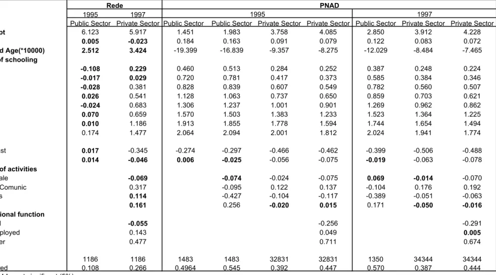
V.1 Log-earnings regressions results

The parametric approach depends on the estimates of Mincer equations for the six log-earnings distributions available (Rede, PNAD Private, and PNAD Public, for 1995 and 1997). Table 3 presents the results of these estimations.

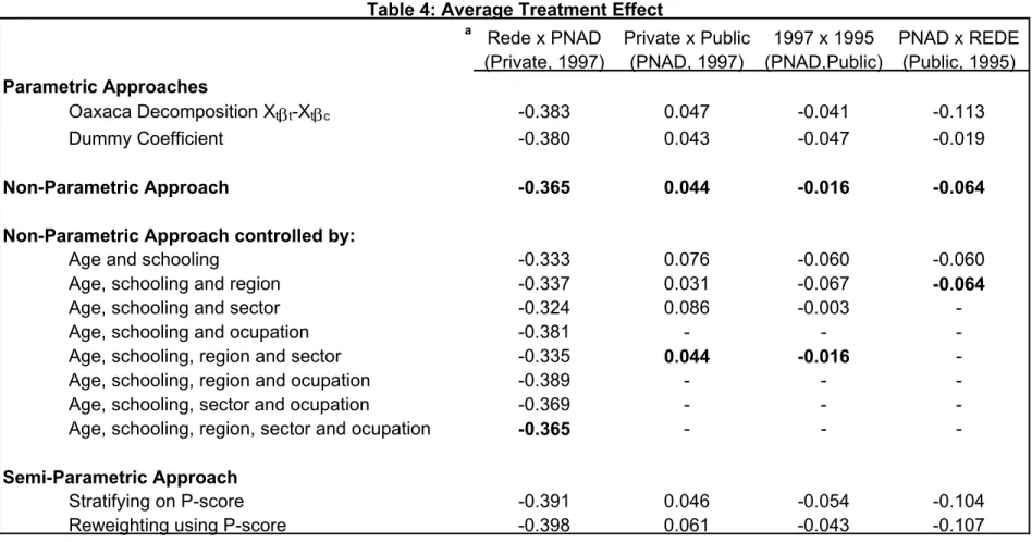
V.2 Average Treatment Effects and Counterfactual Distributions

Table 4 presents the estimates of the average treatment effect (ATE) when comparing the 4 pairs of earnings distributions, which constitute the 4 intermediate steps proposed in Case 1 at the end of Section III for decomposing the total wage gap. We estimate the ATE, controlling for observable characteristics, by using the parametric, semi-parametric and non-parametric methods discussed in the previous Section. In particular, we also show how the results for the nonparametric approach vary as we add more controls. The idea is to test how robust are the results with respect to the choice of matching techniques. The ATE gives the difference between the average actual earnings of the treatment group and the one that would prevail if the characteristics of the treatment group were evaluated at the prices of the control group.

The first column of the Table presents the results for the first step of the decomposition, which is the most important for the objective of this paper. The first column compares the two distributions of private sector workers in 1997: the former Rede workers (the treatment group) and PNAD workers (the control group). The question being posed is: what would be the earnings of a Rede worker if his characteristics were valued as a typical PNAD private sector worker?

The result is a negative and large ATE, which is very robust with respect to the method used. The estimates vary in the range [-0.398, -0,324]. The most flexible method, the nonparametric approach, controlling for age, schooling, region, sector and occupation, gives an estimate of –0.365. That is, according to this estimate, the average log-earnings of a former Rede worker would be 0.365 higher than his actual log-earnings, if his characteristics were evaluated as in the private sector as a whole. This corresponds to average actual earnings 30.6% lower than the average of the counterfactual distribution. These former Rede workers, not only suffered a decrease in their actual earnings with respect to what they were receiving at Rede, but also observed a considerable decrease with respect to their best estimate of what they would make in the private sector, given their observable characteristics.

The second column of Table 4 presents the results for the second pair of distributions, the ATE of being in the private sector (treatment group) in 1997 when using the public sector in the same year as a control group. The ATE is also very robust to the choice of methods, varying from 0.027 to 0.086. The nonparametric method, when using all available controls, gives an estimate of 0.044. This means that the private sector is paying on average 4.5% more than the public sector when one controls for observable characteristics.

were better paid in 1995, on average, than equally qualified workers in the public sector as a whole – as measured by their observable characteristics. The estimates range from –0.113 to -0.064, the estimate given by the nonparametric approach when using controls for age, schooling and region.

Comment box-plots (Figures 3a to 3d).

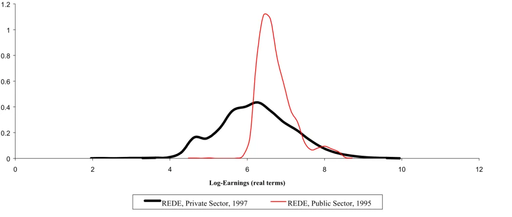
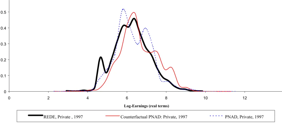
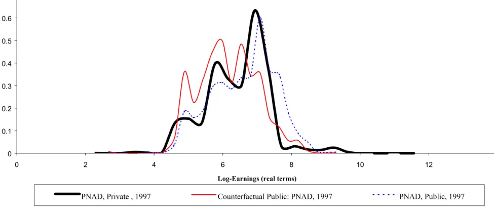
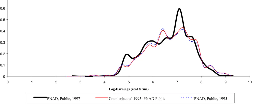
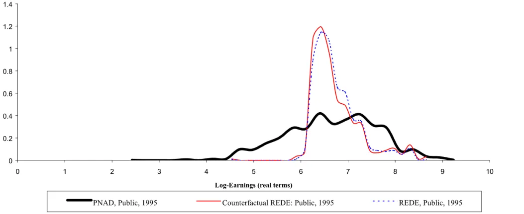
Figures 4a to 4d extend the analysis to the comparison of the complete distributions for each of the 4 pairs discussed above. Each graph displays the actual distribution of the treatment group (thick and black line), the control group (dotted and blue line), and the counterfactual distribution (thin and red line). As above, the counterfactual distribution gives the prices of the control group to the characteristics of the treatment group.

Figure 4a shows that the counterfactual distribution of evaluating Rede workers characteristics at the prices of the private sector is almost entirely to the right of the actual earnings distribution of these workers in the private sector. According to the counterfactual distribution, there would be a much smaller proportion of workers receiving less than 2 minimum wages and much more receiving higher wages.

Figure 4b, on the other hand, shows that the counterfactual distribution of evaluating private sector workers characteristics at the prices of the public sector in 1997 is almost entirely to the left of the actual earnings distribution of private sector workers.

Figure 4d shows how different are the counterfactual distribution of evaluating public sector workers characteristics at the prices paid at Rede in 1995 and the actual distribution of public sector workers. The counterfactual distribution is much more compact, tracking very closely the actual Rede earnings distribution. In fact, this Figure illustrates that the data set does not have enough variation in the covariates to simulate the differences from workers at Rede and the public sector as a whole.

V.3 The Treatment Effect by Human Capital

The main result of the previous Section was that the whole distribution of earnings of former Rede workers is at the left of what would be expected given their characteristics, the counterfactual distribution. In order to help interpreting this result, this sub-section attempts to identify a pattern of treatment effects by some observable characteristics. In particular, we measure the treatment effect by a human capital index, which can be constructed at the individual level as discussed in Section IV.2. The question being posed is: who lost more from what was expected, those with high or low human capital.

Figures 5a to 5d plot the treatment effects for the 4 pairs of distributions against the human capital index. Figure 5a shows that the treatment effect of being a former Rede worker affected negatively all workers. However, the effect was larger (in absolute value) for those with high human capital than for those with low human capital.

Standard human capital theory can lead us to interpret this result in either an optimistic or a pessimistic way. The optimistic view is that those with high general human capital tend to invest more in specific human capital. Since this investment takes time to generate returns, we are observing these workers at the investment period and we should expect their earnings to increase in the future. Pessimists could argue that the value of general human capital has depreciated after so much time in a public firm, and that we could be observing permanent reductions in their earnings, without any tendency to a future increase. Pessimists could also argue that a possible public sector stigma effect could be higher for those with high human capital.

human capital have a negative treatment effect. That is, the private sector is paying them less than the public sector when controlling for observable characteristics. This is somewhat surprising, since one would expect that the public sector in Brazil remunerate better than the private sector the observable characteristics of those with low human capital, and not the opposite.

Finally, Figure 5d shows a huge dispersion of treatment effects of being a former Rede worker against being in the public sector as a whole, as already suggested by Figure 4d. Treatment effects increase substantially with the level of human capital.

The advantage of the human capital index is its continuity. The disadvantage is the difficulty to disentangle the effects of age and schooling. In order to separately analyze the effects of education, Figures 6a to 6d use the discrete levels of schooling as the human capital variable. One can basically observe the same patterns as in Figures 5a-5d, which corroborates the interpretations attributing a major role to schooling variables in the human capital index.

V. Concluding remarks

[To be written]

References [check]

Amadeo, E., Camargo, J.M., and Gonzaga, G. (1998), “Projeto de Pesquisa da Situação Laboral dos Empregados que Aderiram ao Plano de Incentivo ao Desligamento da RFFSA, Nono Relatório de Atividades”. PUC-Rio, Rio de Janeiro, June.

Angrist, J. D. and A. B. Krueger (1999), “Empirical Strategies in Labor Economics”. In:

Ashenfelter, O. and D. Card (eds.) Handbook of Labor Economics, vol. 3A, 1277-1366.

Bourguignon, F. (1979) “Decomposable Income Inequality Measures”, Econometrica, 47(4):

901-920, July.

Carneiro, F. and Gill, I. (1999) “Public Sector Downsizing in Brazil”, Texto para Discussão No.6, Série Economia, UCB, Brasília, August.

Dehejia, R. H. and S. Wahba (1998), “Propensity Score Matching Methods for Non-experimental

Causal Studies”NBER Working Paper W6829.

Dehejia, R. H. and S. Wahba (1999), “Causal Effects in Non-Experimental Studies: Re-Evaluating

the Evaluation of Training Programs”, Journal of the American Statistical Association,

Vol. 94, no. 448: 1053-1062

Foguel, M., Gill, I., Mendonça, R. and Barros, R. P. (2000), “The Public-Private Wage Gap in

Brazil”, Revista Brasileira de Economia, 54(4): 433-472, October- December.

Hahn, J. (1998), “On the role of the propensity score in efficient semiparametric estimation of

average treatment effects”, Econometrica, vol. 66, no. 2, (March, 1998), 315-331.

Heckman, J. (1990), “Varieties of Selection Bias”, American Economic Review, 80, pp. 313-318.

Heckman, J., Ichimura, H., and Todd, P. (1998), “Matching as an Econometric Evaluation Estimator”, The Review of Economic Studies, vol. 65, no. 2, (April, 1998), 261-294.

Juhn, C., Murphy, K. and Pierce, B. (1993), “Wage Inequality and the Rise in Returns to Skill”,

Journal of Political Economy, 101(3): 410-442, June.

Powell, J. (1994), “Estimation of Semiparametric Models”, Handbook of Econometrics, vol.4, edited by R. Engle and D. McFadden, Elsevier Science BV.

Rama, M. (1999) “Public Sector Downsizing: An Introduction”, The World Bank Economic

Review, 13(1): 1-22, January.

Rosenbaum, P. and D. Rubin (1983), “The Central Role of the Propensity Score in Observational

Studies for Causal Effects.” Biometrika, 70(1), 41-55.

Rosenbaum, P. and D. Rubin (1984), “Reducing Bias in Observational Studies Using

Sub-classification on the Propensity Score.” Journal of the American Statistical Association,

516-524, September

Rubin, D. (1977) “Assignment to a Treatment Group on the Basis of a Covariate”, Journal of

1995 1997

Public Sector Private Sector Public Sector Private Sector Public Sector Private Sector

Log-earnings 6.74 6.25 6.63 6.22 6.62 6.22

Age 39.84 38.83 39.48 38.87

Years of schooling

0-3 12.7% 23.3% 11.8% 21.9%

4 12.9% 22.3% 8.8% 19.5%

5-7 7.2% 14.4% 7.0% 15.7%

8 8.9% 11.6% 7.8% 12.2%

9-10 4.2% 4.2% 4.3% 4.4%

11 23.6% 14.1% 27.0% 15.6%

12-14 7.8% 2.7% 8.5% 2.8%

15 13.4% 4.3% 13.1% 4.3%

16 or + 9.5% 3.1% 11.7% 3.5%

Region

Northeast 24.5% 19.3% 21.7% 19.6%

South 19.8% 17.9% 20.1% 18.1%

Southeast/Middle West 55.7% 62.8% 58.3% 62.2%

Sector of activities

Industry 12.3% 36.8% 40.6% 32.4% 39.8%

Wholesale 29.9% 1.4% 19.4% 1.2% 19.3%

Transp/Comunic 11.9% 20.5% 9.7% 19.2% 10.0%

Services 39.2% 24.3% 27.5% 31.3% 28.3%

Others 6.7% 17.0% 2.8% 15.9% 2.5%

Ocupational function

Formal 27.6% 90.5% 47.2% 85.5% 45.8%

Informal 12.6% 9.6% 13.0% 14.5% 14.2%

Self-employed 37.2% 31.1% 31.3%

Employer 22.7% 8.6% 8.8%

# of observations 1,483 32,831 1,350 34,344

18.5% 66.5% Rede 971.51 16.3% 4.3% 835.46 15.5% 15.0% 1997 PNAD 814.86 818.71 1140.19 1173.26 1995 1,186 40.58

Table 1: Summary statistics (Rede & PNAD)

10.5% 23.4% 4.9% 11.2% 5.1% 8.9%

a

Private x Public

Rede x PNAD

Private x Public

1997 x 1995

PNAD x REDE

(Rede)

(Private, 1997)

(PNAD, 1997)

(PNAD,Public)

(Public, 1995)

Total Wage Gap

-0.488

0.036

-0.401

-0.011

-0.112

note:

a

- treatment x control

1995 1997

Public Sector Private Sector Public Sector Public Sector Private Sector Private Sector Public Sector Private Sector Private Sector

Intercept 6.123 5.917 1.451 1.983 3.758 4.085 2.850 3.912 4.228

Age 0.005 -0.023 0.184 0.163 0.091 0.079 0.122 0.083 0.072

Squared Age(*10000) 2.512 3.424 -19.399 -16.839 -9.357 -8.275 -12.029 -8.484 -7.465

Years of schooling

4 -0.108 0.229 0.460 0.513 0.284 0.252 0.387 0.248 0.224

5-7 -0.017 0.029 0.720 0.781 0.417 0.373 0.585 0.384 0.346

8 -0.028 0.381 0.828 0.839 0.607 0.549 0.782 0.560 0.507

9-10 0.026 0.541 1.128 1.063 0.737 0.650 0.859 0.703 0.621

11 -0.024 0.683 1.306 1.237 1.001 0.901 1.269 0.962 0.862

12-14 0.070 0.659 1.570 1.503 1.383 1.233 1.523 1.364 1.225

15 0.010 1.186 1.913 1.855 1.778 1.594 1.744 1.654 1.494

16 or + 0.174 1.477 2.064 2.094 2.001 1.812 2.024 1.941 1.774

Region

Northeast 0.017 -0.345 -0.274 -0.297 -0.466 -0.462 -0.399 -0.506 -0.488

South 0.014 -0.046 0.006 -0.025 -0.056 -0.075 -0.019 -0.063 -0.078

Sector of activities

Wholesale -0.069 -0.074 -0.024 -0.075 0.069 -0.014 -0.070

Transp/Comunic 0.317 -0.095 0.122 0.137 -0.104 0.176 0.192

Services 0.114 -0.427 -0.104 -0.117 -0.389 -0.051 -0.063

Others 0.161 0.256 -0.020 0.015 0.171 -0.050 -0.016

Ocupational function

Informal -0.055 -0.256 -0.291

Self-employed 0.143 0.049 0.005

Employer 0.477 0.711 0.674

#obs 1186 1186 1483 1483 32831 32831 1350 34344 34344

R squared 0.108 0.266 0.4964 0.545 0.392 0.447 0.570 0.387 0.444

note: bold = not significant (5%)

Table 3: Log-Earnings regression results

Rede PNAD

a

Rede x PNAD Private x Public 1997 x 1995 PNAD x REDE

(Private, 1997) (PNAD, 1997) (PNAD,Public) (Public, 1995)

Parametric Approaches

Oaxaca Decomposition Xtβt-Xtβc -0.383 0.047 -0.041 -0.113

Dummy Coefficient -0.380 0.043 -0.047 -0.019

Non-Parametric Approach -0.365 0.044 -0.016 -0.064

Non-Parametric Approach controlled by:

Age and schooling -0.333 0.076 -0.060 -0.060

Age, schooling and region -0.337 0.031 -0.067 -0.064

Age, schooling and sector -0.324 0.086 -0.003

-Age, schooling and ocupation -0.381 - -

-Age, schooling, region and sector -0.335 0.044 -0.016

-Age, schooling, region and ocupation -0.389 - -

-Age, schooling, sector and ocupation -0.369 - -

-Age, schooling, region, sector and ocupation -0.365 - -

-Semi-Parametric Approach

Stratifying on P-score -0.391 0.046 -0.054 -0.104

Reweighting using P-score -0.398 0.061 -0.043 -0.107

note:

a

- treatment x control

Figure 1: Log-Earnings Density Function: REDE Employees: after and before leaving the public sector

0 0.2 0.4 0.6 0.8 1 1.2

0 2 4 6 8 10 12

Log-Earnings (real terms)

Figure 2a.

Age Groups (REDE)

Fraction Age Groups 25-29 30-34 35-39 40-44 45-49 50-54 55-59 60-64 0 .316189

Age Groups (PNAD, Public Sector, 1997)

Fraction Age Groups 25-29 30-34 35-39 40-44 45-49 50-54 55-59 60-64 0 .226654

Age Groups (PNAD, Private Sector, 1997)

Fraction Age Groups 25-29 30-34 35-39 40-44 45-49 50-54 55-59 60-64 0 .199948 Figure 2b.

Years of schooling (REDE)

Fraction

Years of schooling

0-3 4 5-7 8 9-10 11 12-14 15

16 or +

0

.234401

Years of schooling (PNAD, Public Sector, 1997)

Fraction

Years of schooling

0-3 4 5-7 8 9-10 11 12-14 15

16 or +

0

.269538

Years of schooling (PNAD, Private Sector, 1997)

Fraction

Years of schooling

0-3 4 5-7 8 9-10 11 12-14 15

16 or +

0

Figure 2c.

Sector of activities (REDE)

Fraction

Sector of activities

Industry Wholesal Transp/C Services Others 0 .392074

Sector of activities (PNAD, Public Sector, 1997)

Fraction

Sector of activities

Industry Wholesal Transp/C Services Others 0 .324362

Sector of activities (PNAD, Private Sector, 1997)

Fraction

Sector of activities

Industry Wholesal Transp/C Services Others 0 .398234 Figure 2d.

Ocupational function (REDE)

Fraction Ocupational function Formal Informal Self-emp Employer 0 .371838

Ocupational function (PNAD, Public Sector, 1997)

Fraction Ocupational function Formal Informal 0 .855304

Ocupational function (PNAD, Private Sector, 1997)

Figure 4a: Log-Earnings Density Function: REDE X PNAD (Private Sector, 1997)

0 0.1 0.2 0.3 0.4 0.5 0.6

0 2 4 6 8 10 12 14

Log-Earnings (real terms)

Figure 4b: Log-Earnings Density Function: Private X Public Sectors (PNAD, 1997)

0 0.1 0.2 0.3 0.4 0.5 0.6 0.7

0 2 4 6 8 10 12 14

Log-Earnings (real terms)

Figure 4c: Log-Earnings Density Function: 1997 X 1995 (PNAD, Public Sector)

0 0.1 0.2 0.3 0.4 0.5 0.6 0.7

0 1 2 3 4 5 6 7 8 9 10

Log-Earnings (real terms)

Figure 4d: Log-Earnings Density Function: PNAD X REDE (Public Sector, 1995)

0 0.2 0.4 0.6 0.8 1 1.2 1.4

0 1 2 3 4 5 6 7 8 9 10

Log-Earnings (real terms)