Clinical Trial Adaptation by Matching Evidence in Complementary Patient Sub-groups of Auxiliary Blinding Questionnaire Responses.

(1)

Clinical Trial Adaptation by Matching

Evidence in Complementary Patient

Sub-groups of Auxiliary Blinding Questionnaire

Responses

Ognjen Arandjelović_*

Centre for Pattern Recognition and Data Analytics, School of Information Technology, Deakin University, Geelong, Victoria, Australia

*[email protected]

Abstract

Clinical trial adaptation refers to any adjustment of the trial protocol after the onset of the trial. Such adjustment may take on various forms, including the change in the dose of administered medicines, the frequency of administering an intervention, the number of trial participants, or the duration of the trial, to name just some possibilities. The main goal is to make the process of introducing new medical interventions to patients more efficient, either by reducing the cost or the time associated with evaluating their safety and efficacy. The principal challenge, which is an outstanding research problem, is to be found in the question of how adaptation should be performed so as to minimize the chance of distorting the out-come of the trial. In this paper we propose a novel method for achieving this. Unlike most of the previously published work, our approach focuses on trial adaptation by sample size adjustment i.e. by reducing the number of trial participants in a statistically informed manner. We adopt a stratification framework recently proposed for the analysis of trial outcomes in the presence of imperfect blinding and based on the administration of a generic auxiliary questionnaire that allows the participants to express their belief concerning the assigned intervention (treatment or control). We show that this data, together with the primary mea-sured variables, can be used to make the probabilistically optimal choice of the particular sub-group a participant should be removed from if trial size reduction is desired. Extensive experiments on a series of simulated trials are used to illustrate the effectiveness of our method.

Introduction

Robust evaluation is a crucial component in the process of introducing new medical interven-tions. Amongst others, these include newly developed medications, novel means of administer-ing known treatments, new screenadminister-ing procedures, diagnostic methodologies,

physio-a11111

OPEN ACCESS

Citation:ArandjelovićO (2015) Clinical Trial Adaptation by Matching Evidence in Complementary Patient Sub-groups of Auxiliary Blinding

Questionnaire Responses. PLoS ONE 10(7): e0131524. doi:10.1371/journal.pone.0131524

Academic Editor:Massimo Pietropaolo, Baylor College of Medicine, UNITED STATES

Received:May 13, 2014

Accepted:June 3, 2015

Published:July 10, 2015

Creative Commons Attribution License, which permits unrestricted use, distribution, and reproduction in any medium, provided the original author and source are credited.

Data Availability Statement:All relevant data are within the paper.

Funding:The author has no support or funding to report.

(2)

therapeutical manipulations, and many others. Such evaluations usually take on the form of a controlled clinical trial (or a series thereof), the framework widely accepted as best suited for a

rigourous statistical analysis of the effects of interest [1–3] (for a related discussion and critique

also see [4]). Driven both by legislating bodies, as well as the scientific community and the

pub-lic, the standards that the assessment of novel interventions are expected to meet continue to rise. Generally, this necessitates trials which employ larger sample sizes and which perform assessment over longer periods of time. A series of practical challenges emerge as a conse-quence. Increasing the number of individuals in a trial can be difficult because some trials necessitate that participants meet specific criteria; volunteers are also less likely to commit to

participation over extended periods of time. The financial impact is another major issue—both

the increase in the duration of a trial and the number of participants result in additional cost to an already expensive process. In response to these challenges, the use of adaptive trials has

emerged as a potential solution [5–9].

The key idea underlying the concept of an adaptive trial design is that instead of fixing the parameters of a trial before its onset, greater efficiency can be achieved by adjusting them as

the trial progresses [10]. For example, the trial sample size (e.g. the number of participants in a

trial), treatment dose or frequency, or the duration of the trial may be increased or decreased

depending on the accumulated evidence [11–13].

Proposed method overview

The method for trial adaptation we describe in this paper extends the analysis presented in [14]

which has been greatly influenced by recent work on the analysis of imperfectly blinded clinical

trials [15,16]. Its key contribution was to introduce the idea of trial outcome analysis by patient

sub-groups which comprise trial participants matched by the administered intervention (treat-ment or control) and their responses to an auxiliary questionnaire in which the participants are asked to express their belief regarding their assignment intervention in the closed-form (see

Auxiliary data collectionfor a summary of the adopted sub-group stratification method and

the original paper [16] for full detail). This framework was shown to be suitable for robust

inference in the presence of“unblinding”in a trial [16,17]. The method proposed in the

pres-ent paper emerges from the realization that the same framework can be used for trial adapta-tion by providing informaadapta-tion which can be used to make a statistically informed selecadapta-tion of the trial participants which can be dropped from the trial before its completion, without signifi-cantly affecting the trial outcome. Thus, the proposed approach falls under the category of trial

adaptations by“amending sample size”, in contrast to“dose finding”or“response adapting”

methods which dominate previous work [13].

In [16] it was shown that the analysis of a trial’s outcome should be performed by

aggregat-ing evidence provided by matched participant sub-groups, where two sub-groups are matched if they contain participants who were administered different interventions but nonetheless had the same responses in the auxiliary questionnaire. Therefore, our idea advanced here is that an informed trial sample size reduction can be made by computing which matched sub-group

pair’s contribution of useful information is affected the least with the removal of a certain

num-ber of participants from one of its groups.

Contrast with previous work. Before introducing the proposed method in detail, it is worthwhile emphasizing two fundamental aspects in which it differs from the methods previ-ously described in the literature. The first difference concerns the nature of the statistical framework which underlies our approach. While the use of Bayesian techniques has become

increasingly common in medical statistics [18–22], and perhaps particularly so in the context

(3)

work on trial adaptation by sample size adjustment adopts the frequentist paradigm [30–32]. These methods follow the following general pattern: a particular null hypothesis is formulated which is then rejected or accepted using a suitable statistic and the desired confidence

require-ment (a good review is provided by Jennison and Turnbull [33]). In contrast, the method

described in this paper is thoroughly Bayesian in nature.

The second major conceptual novelty of the proposed method lies in the question it seeks to answer. Previous work on trial adaptation by sample size adjustment addresses the question of

whetherthe sample size can be reduced while maintaining a certain level of statistical

signifi-cance of the trial’s outcome. In contrast, the present work is the first to ask a complementary

question ofwhichparticular individuals in the sample should be removed from the trial once

the decision of sample size reduction has been made. Thus, the proposed method should not be seen as an alternative to the any of the previously proposed methods but rather as a comple-mentary element of the same framework.

Auxiliary data collection

The type of auxiliary data collection we utilize in this work was originally proposed for the

assessment of blinding in clinical trials [34]. Since then it has been adopted for the same

pur-pose in a number of subsequent works [16,35–37] (also see [38] for related commentary).

With the exception of [16], in all previous work the questionnaire is employed after the trial

has ended (for discussions on the timing of the questionnaire see [16,39,40]). The

question-naire allows the trial participants to express their belief on the nature of the intervention they have been administered (control or treatment) using a fixed number of choices. The most com-monly used, coarse-grained questionnaire admits the following three choices:

Choice 1: the patient believes that he/she was administered the control intervention (i.e. control group membership),

Choice 2: the patient believes that he/she was administered the treatment intervention (i.e. treatment group membership), and

Choice 3: the patient is undecided about the nature of the treatment he/she was administered

(the“don’t know”response).

Extensions of this scheme which attempt to harness more detailed information have also been

used, for example allowing the participants to quantify the conviction of their belief as“weak”

or“strong”. In that case, the questionnaire would offer five choices:

Choice 1: the patientstronglybelieves that he/she was administered the control intervention,

Choice 2: the patientweaklybelieves that he/she was administered the control intervention,

Choice 3: the patient is undecided about the nature of the treatment he/she was administered,

Choice 4: the patientweaklybelieves that he/she was administered the treatment intervention,

and

Choice 5: the patientstronglybelieves that he/she was administered the treatment intervention.

More granular auxiliary data choices have the potential of providing a more accurate picture of the extent of blinding. However, depending on the statistical model used, this advantage may come at the cost of reduced statistical significance for each of the response sub-groups. The

evi-dence on the capacity of a human’s working memory [41] suggests that the number of

(4)

Matching sub-groups outcome model

In the general case, the effectiveness of a particular intervention in a trial participant depends

on the inherent effects of the intervention, as well as the participant’s expectations (conscious

or not). Thus, as in [16], in the interpretation of trial results, we separately consider each

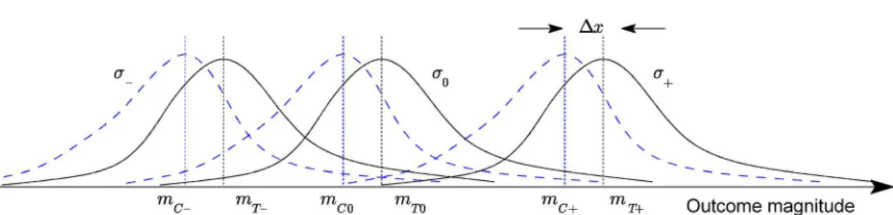
popu-lation of participants which share the same combination of the type of intervention and the expressed belief regarding this group assignment. For example, when a 3-tier questionnaire is used in a trial comparing the administration of the treatment of interest and control, we recog-nize 3×2 = 6 auxiliary data sub-groups:

Sub-group 1: participants of the control group who believe they were assigned to the control

group (sub-groupGC−),

Sub-group 2: participants of the control group who are unsure of their group assignment

(sub-groupGC0),

Sub-group 3: participants of the control group who believe they were assigned to the treatment

group (sub-groupGC+),

Sub-group 4: participants of the treatment group who believe they were assigned to the control

group (sub-groupGT−),

Sub-group 5: participants of the treatment group who are unsure of their group assignment

(sub-groupGT0), and

Sub-group 6: participants of the treatment group who believe they were assigned to the

treat-ment group (sub-groupGT+).

This is illustrated conceptually inFig 1. In the general case, for anN-tier questionnaire andM

different intervention types, we can distinguish betweenN×Mdistinct sub-groups of

participants.

The key idea underlying the method proposed in [16] is that because the outcome of an

intervention depends on both the inherent effects of the intervention and the participants’

expectations, the effectiveness should be inferred in a like-for-like fashion. In other words, the response observed in, say, the sub-group of participants assigned to the control group whose feedback professes belief in the control group assignment should be compared with the response of only the sub-group of the treatment group who equally professed belief in the

Fig 1. Adopted statistical model for a three-tier feedback questionnaire (conceptual illustration)_—the probability densities of the measured trial

outcome across the three control (solid lines) and treatment sub-groups (dotted lines).Diagram reproduced with permission.

(5)

control group assignment. Similarly, the“don’t know”sub-groups should be compared only with each other, as should the sub-groups corresponding to the belief in the treatment assign-ment. Ideas similar in spirit were expressed by Berger in the consideration of the related

prob-lem of so-called selection bias and specifically the Berger-Exner test [42].

Sub-group selection

The primary aim of the statistical framework described in [16] is to facilitate an analysis of trial

data robust to the presence of partial or full unblinding of patients, or indeed patient precon-ceptions which too may affect the measured outcomes. Herein we propose to exploit and extend this framework to guide the choice of which patients are removed from the trial after its onset, in a manner which minimizes the loss of statistical significance of the ultimate

outcomes.

At the onset of the trial, the trial should be randomized according to the current best clinical

practice; this problem is comprehensively covered in the influential work by Berger [42]. If a

reduction in the number of trial participants was attempted at this stage, by the very definition of a properly randomized trial, statistically speaking there is no reason to prefer the removal of any particular subject (or indeed a set of subjects) over another. Instead, any trial size adapta-tion must be performed at a later stage after some meaningful differentiaadapta-tion between subjects

takes place [43–45].

The most obvious measurable differentiation that takes place between patients as the trial

progresses is that of the outcomes of primary interest in the trial (the“response”). This

differ-entiation may allow for a statistically informed choice to be made about which trial participants can be dropped from the trial in a manner which minimizes the expected distortion of the ulti-mate findings. For example, this can be done by seeking to preserve the distribution of mea-sured outcomes within a group (treatment or control) but with the constraint of a smaller number of participants; indeed, our approach partially exploits this idea as will be explained in detail shortly. However, our key contribution lies in a more innovative approach, which exploits additional, yet readily collected discriminative information. The proposed approach not only minimizes the effect of smaller participant groups but also ensures that no uninten-tional bias is injected due to imperfect blinding. Recall that the problem of inference robust to

imperfect blinding should always be considered—as stated earlier, blinding can only be

attempted with respect to those variables of the trial which have been identified as revealing of the administered treatment, and even for the explicitly identified variables it is fundamentally impossible to ensure that absolute blinding is achieved.

Our idea is to administer an auxiliary questionnaire of the form described in [34,35] (which

is normally administered after the trial in the work on blinding assessment) every time an

adaptation of the trial group size (i.e. reduction thereof) is sought. Just like in [16], this leads to

the differentiation of each group of participants (control or treatment) into sub-groups, based on their belief regarding their group assignment. In general, this means that even if no partici-pants are removed from the trial, a participant may change his/her sub-group membership

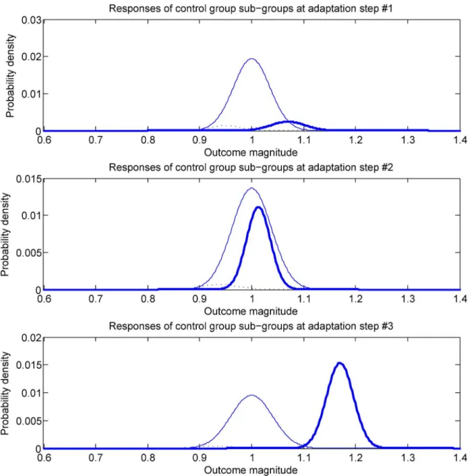
sta-tus. This is illustrated conceptually inFig 2. The first time an auxiliary questionnaire is

(6)

sub-group has changed, as do the associated treatment response statistics. A similar observa-tion can be made with respect to the third and the last snapshot pictured in the figure

(bottom-most plot). This sort of a development would not be unexpected—if the treatment is effective,

as the trial progresses there will be an increase in the number of treatment group participants who observe and correctly interpret these changes (note that this also means that there will be an associated increase in the number of participants who may exhibit an additional positive effect from the fortunate realization that they are receiving the studied treatment intervention, rather than the control intervention). That being said, it should be emphasized that no Fig 2. A conceptual illustration on a hypothetical example of the phenomenon whereby trial participants change their sub-group membership

(recall that each sub-group is defined by its members_’intervention assignmentandauxiliary questionnaire responses).This is quite likely to occur

when the effects of the treatment are very readily apparent but various other mechanisms can act so as to cause a non-zero and changing sub-group flux.

(7)

assumption on the statistics of sub-group memberships or their relative sizes is made in the

proposed method. The example inFig 2is merely used for illustrative purposes.

The question is: how does this differentiation of patients by auxiliary data sub-groups help us make a statistically robust choice of which participants in the trial should be preferentially dropped if a reduction in the trial size is sought? To answer this question, recall the main prem-ise of [16]:

“The key idea [. . .] is that it is meaningful to compare only the corresponding treatment

and control participant sub-groups, that is, sub-groups matched by their auxiliary

responses.”

Each sub-group comparison contributes information used to infer the probability density of the differential effects of the treatment. We can then reformulate the original question as: from which matching sub-group pair should participants be preferentially dismissed from further consideration so as to best preserve the information contribution from all sub-groups?

Consider how the information on the differential effects between a single pair of matching sub-groups is inferred. In its general form, we can estimate some distance between the distribu-tions of the two sub-groups using a Bayesian approach. Indeed, Bayesian analysis based meth-ods have in recent years been continually gaining acceptance across the clinical community

[44]. In brief, the key idea is to“integrate out”the unknown latent parameters of the two

distri-butions. Expressed formally:

r_¼

Z

Y_c

Z

Y_t

rðpcðx;YcÞ;ptðx;YtÞÞ

|fflfflfflfflfflfflfflfflfflfflfflfflfflfflfflfflffl{zfflfflfflfflfflfflfflfflfflfflfflfflfflfflfflfflffl}

Distance between distributions for specific parameter values

pðY

cjDcÞpðYtjDtÞ

|fflfflfflfflfflfflfflfflfflfflfflfflfflffl{zfflfflfflfflfflfflfflfflfflfflfflfflfflffl}

Probability of parameters conditioned on observations

pðY cÞpðYtÞ

|fflfflfflfflfflfflfflffl{zfflfflfflfflfflfflfflffl}

Parameter priors dY

t dYc ð1Þ

whereΘ_c_andΘ_t_{are the sets of variables parameterizing the two corresponding distributions}

pc(x;Θ

c) andpt(x;Θt),p(Θc) andp(Θt) the parameter priors,ρ(pc(x;Θc),pt(x;Θt)) a particular

dis-tance function (e.g. the Kullback-Leibler divergence [46], Bhattacharyya [47] or Hellinger

dis-tances [48], or indeed the posterior of the difference of means used in [16]), andDcandDtthe

measured trial outcomes (such as the amount of fat loss in a fat loss trial, the reduction in blood plasma LDL in a statin trial etc).

Note that by changing (reducing) the number of participants in one of the groups, the only

affected term on the right hand side ofEq (1)is one of the likelihood terms,p(Θ

cjDc) orp

(Θ_t_j_Dt_{). Seen another way, a change in the number of participants in the trial changes the}

weightingof the product of the distance termρ(pc(x;Θ

c),pt(x;Θt)) and the priorsp(Θc)p(Θt).

Our idea is then to choose to remove a trial participant from that sub-group which produces

the smallest change in the estimateρ. However, it is not clear how this may be achieved, since

it is the size of the setDcthat is changing (so, for example, treatingDcandDtas vectors andfas

a function of vectors would not achieve the desired aim). Examining the sensitivity ofρwith

the removal of each datum (i.e. trial participant) fromDcandDtis also unsatisfactory since the

problem does not lend itself to a greedy strategy: the optimal choice of whichnremtrial

partici-pants to drop from the trial cannot be made by makingnremoptimal choices of whichone

par-ticipant to drop. An approach following this direction but attempting to examine all possible

sets of sizenremwould encounter computational tractability obstacles since this problem is

NP-complete. The alternative which we propose is to consider and compare the magnitudes of

par-tial derivatives ofρwith respect to the sizes of data setsDcandDt, but with an important

(8)

ofDcandDt. Formalizing this, we compute:

E @r

@nc

Dc

and E @r

@nt

Dt

; ð2Þ

whereE[ρ]DcandE[ρ]Dtare respectively the expected values ofρacross the space of

possi-ble observations inDcandDt(each with a uniform prior, as before). ThusE[ρ]DcandE[ρ]Dt

are functions of two scalars, the sizesncandntof setsDcandDti.e. the numbers of members of

the corresponding sub-groups.

The proposed solution is not only theoretically justified but it also lends itself to simple and

efficient implementation. Since the expected valuesE[ρ]DcandE[ρ

_]

Dtare evaluated over sets

DcandDt, inEq (1)the only term affected isp(Θ

cjDc)p(ΘtjDt), so the solution is readily

obtained as a closed form expression. Equally, the integration is readily performed using one of

the standard Markov chain Monte Carlo integration methods [49].

Application example

In order to illustrate how the described idea could be applied in practice, we now consider one specific example of the distance function discussed in the previous section and show how the mathematical results needed to implement the proposed methodology can be derived or esti-mated. Readers who are not interested in full technical detail of this nature can skip this section

and proceed toNote on practical applicationwithout loss in continuity.

Let the trial observation data in two matching sub-groups be drawn from the random

vari-ablesXcandXt, which are appropriately modelled using log-normal distributions [50]:

Xt 1

xs_t exp

lnx mt

2s2 t

ð3Þ

and

Xc 1

xs_c exp

lnx mc

2s2 c

ð4Þ

The next step is to choose an appropriate distance functionρinEq (1). In practice, this choice

would be governed by the goals of the study. Herein, for illustrative purposes we chooseρto be

the probability that a patient will do better when the treatment rather than the control inter-vention is administered:

rðptðx;YtÞ;pcðy;YcÞÞ ¼

Z 1

0

Z x

0

ptðx;YtÞpcðy;YcÞdy dx

whereΘ_c_{= (}_mc_,_σ_c_{) and}Θ_t_{= (}_mt_,_σ_t_{) are the mean and standard deviation parameters specifying}

the corresponding log-normal distributions.

r / Z 1 0 Z 1 1 Z 1 0 Z 1 1 Z 1 0 Z x 0 n

ptðxjmt;stÞpðmt;stÞdx dmt dstpcðyjmc;scÞ pðmc;scÞdy dmc dsc o

ð5Þ

Making the usual substitution wherebyexis substituted forx(and similarlyeyfory), which

(9)

(just as in [16]) leads to the following expression

r _/

Z1 0 Z1 1 Z1 0 Z1 1 Z1 0 Zx 0 s 1 t e ðx mtÞ2

2s2

t s N t e

Pnt i¼1ðx

ðtÞ

i mtÞ

2 2s2

t dx dm

tdst

s 1 c e

ðx mcÞ2 2s2

c s N c e

Pnc i¼1ðx

ðcÞ

i mcÞ

2 2s2

c dy dm

cdsc ð6Þ

¼

Z1

0

Zx

0

ItðxÞIcðyÞdy dx¼

Z1

0 ItðxÞ

Zx

0

IcðyÞdy dx ð7Þ

where each of the integralsIt(x) andIc(y) has the form:

I¼ Z 1 0 Z 1 1 1 s exp

ðx mÞ2

2s2

1

sn exp

Pn

i¼1ðxi mÞ 2

2s2

dm ds; ð8Þ

{xi} andnstand for either xðcÞi

n o

andncor xðtÞi

n o

andnt, and xðcÞi

n o

(i= 1. . .nc) and xiðtÞ

n o

(i= 1. . .nt) are exponentially transformed measured trial variables. This integral can be evalu-ated by combining the two exponential terms and completing the square of the numerator of

the exponent as in [16] so that:

ðx mÞ2

þX

n

i¼1

ðxi mÞ 2

ðamþbÞ2

þc; ð9Þ

which leads to the following simpliﬁcation ofEq (7):

I/

Z1

0

1

snþ2 exp c

2s2

n o

sds ð10Þ

¼

Z1

0

1

snþ1 exp c

2s2

n o

ds; ð11Þ

where the value of the only non-constant term,c, is:

c¼x2

þX

n

i¼1 xi

2 ðxþ

Pn

i¼1xiÞ 2

nþ1 ð12Þ

¼ðnþ1Þðx 2_þPn

i¼1xi2Þ ðxþ

Pn

i¼1xiÞ 2

nþ1 : ð13Þ

Observing that the form of the integrand inEq (11)matches that of the inverse gamma

dis-tribution:

Gammaðz;a;bÞ ¼ b

a

G_ð_a_Þz a 1

expf b=zg: ð14Þ

whereΓ₍_α_{) is the value of the gamma function at}_α_{. The variable}_z_{and the two parameters of}

(10)

out, leaving the integral proportional to a single non-constant term:

I/c n21: ð15Þ

Notice that the form of this result is very similar to that obtained in [16].

Remembering that the functional form ofcis different for the control and the trial groups

(since it is dependent onxiwhich stands for eitherxðcÞi orx

ðtÞ

i ), and substituting the result from

Eq (15)back intoEq (7)gives the following expression for the distance function:

r_¼

Z1

0

Zx

0

ptðxÞpcðyÞdy dx ð16Þ

/ Z1 0 Zx 0 c nt 1 2 t c nc 1 2

c dy dx ð17Þ

¼ Z1 0 c nt 1 2 t Zx 0 c nc21

c dy dx ð18Þ

Our goal now is to evaluateSc(ρ) andSt(ρ), the sensitivities of the distance function to the

change in the size of respectively the control and the treatment groups. Without loss of

general-ity, let us considerSt(ρ)—the symmetry of the expression inEq (18)makes it trivial to apply

the same process to the computation ofSt(ρ). FromEq (18):

Stðr _{Þ /}

Z1

1

Zx

1

S½ItðxÞIcðyÞdy dx ð19Þ

To evaluateS[It(x)] we will employ the standard chain rule and perform differentiation with

respect tontwhen the corresponding term is a function of the number of treatment

partici-pants but not anyxiðtÞ. On the other hand, as proposed inSub-group selection, to handle those

terms which do depend onxðtÞi (throughct), we will use the expected value of the change in the

term, averaged over all possiblexðtÞi that a unitary decrease inntcan be achieved. Applying this

idea on the expression inEq (8)leads to the following expansion:

S_½ItðxÞ ¼ Z1 0 Z1 1 1 sexp

ðx m_Þ2

2s2

ln_snsexp Pn

i¼1ðxi mÞ 2

2s2

þ_s1n exp Pn

i¼1ðxi mÞ 2

2s2

Pn

i¼1ðxi mÞ 2

2s2_n2

dm ds _ð20Þ

noting that we used the standard result:

d dn

1

sn¼

lns

sn ð21Þ

(11)

expression can be further rearranged, yielding the following, more concise expression:

S½ItðxÞ ¼

Z1

0

Z1

1

lns sn exp

ðx mÞ2

2s2

exp

Pn

i¼1ðxi mÞ 2

2s2

dm ds ð22Þ

Z1

0

Z1

1 1

snþ3_n2 exp

ðx mÞ2

2s2

exp

Pn

i¼1ðxi mÞ 2

2s2

Xn

i¼1

ðxi mÞ 2

dm ds: ð23Þ

Full double integration of the integrands inEq (23)is difficult to perform analytically.

How-ever, one level of integration—with respect tom—is readily achieved. Note that the first term,

as a function ofm, has the same form as the integral inEq (8)which we already evaluated. The

same procedure which uses the completion of the square in the exponential term can be

applied here as well (note that unlike inEq (8)here it is important to keep track of the

multipli-cative constants as these will be different for the second term inEq (23)). The integrand in the

second term can be expressed in the form/(z−λ)2exp−z2dz. This integration is also readily

performed using the standard results:

Z1

1 1

ffiffiffiffiffiffi

2p p z2

exp z

2

2 dz¼1 ð24Þ

and Z1 1 1 ffiffiffiffiffiffi 2p

p exp z

2

2 dz¼1; ð25Þ

and by noting that the integrand is an odd function

Z1

1 1

ffiffiffiffiffiffi

2p

p z exp z

2

2 dz¼0 ð26Þ

A straightforward application of these results toEq (23)leads to the following expression for

the sensitivityS[It(x)] of the integralItto changes in the size of the corresponding sub-group

(the treatment sub-group in a matching pair):

S½ItðxÞ ¼ Z1

0

lns snþ1

s a ffiffiffiffiffiffi 2p p exp c

2s2

n o

ds Z1

0

exp c

2s2

2snþ3_n2 n

s

a 3

þpffiffiffiffiffiffi2ps

a

Xn

i¼1 xi

" #

ds ð27Þ

This result, together with the expression inEq (15), can be substituted intoEq (19)and the

remaining integration performed numerically.

Note on practical application

As demonstrated in the preceding section, it is worth observing that none of the calculations involved make any strong assumptions on the nature of the phenomenon studied i.e. the nature of the outcome data. There are only two elements of the described framework which are subject

to change depending on the trial. These are the distance functionρand the form of the

likeli-hood termsp(Θ_c_j_Dc_{) and}_p₍Θ_t_j_Dt_{), see}_{Eq (1)}_{. In practice, all of these terms are confined to a}

(12)

detail in the previous section can be performeda priori, with only the final numerical

computa-tions (which are not computationally demanding) performed“on the fly”. Consequently, while

the implementation of the proposed approach clearly requires expertise in mathematics and computation, no mathematical expertise or thorough understanding of the details of the algo-rithm need to be expected from the user (e.g. a clinician or a biostatistician). The user would

merely need to select one of a number of possible outcomes of interest (e.g.“effect greater

than”) and set the value of the relevant parameter according to the aims of the study (e.g.

“effect greater than 0.1”), and be automatically presented with the best sample selection and

the corresponding posterior distributions quantifying the uncertainty associated with the

resul-tant outcome. This will be illustrated shortly on simulated examples inEvaluation and

analysis.

From target sub-groups to specific participants

Adopting the framework proposed in [16] whereby the analysis of a trial takes into account

sub-groups of trial participants, which emerge from grouping participants according to their assigned intervention and auxiliary data, thus far we focused on the problem of choosing the sub-group from which participants should be preferentially removed if a reduction in trial size

is sought. The other question which needs to be considered is howspecificsub-group members

are to be chosen, once the target sub-group is identified. Fortunately, the proposed framework makes this a simple task. Recall that the observed trial data within each sub-group is assumed to comprise an identically and independently distributed sample from the underlying

distribu-tion, i.e.xðcÞi Xc(or indeedx

ðtÞ

i Xt). This means that it is sufﬁcient to randomly sample the

set of target sub-group members to select those which can be removed.

The simplicity of the selection process that our approach allows has an additional welcome consequence. Recall that in the proposed method the choice of the target sub-group is made by

comparing differentials inEq (2). It is important to observe that their values are computed for

the initial values ofncandnt. Thus, as the number of participants in either of the sub-groups is

changed, so do the values of the differentials, and thus possibly the optimal sub-group choice.

This is why the removal of participants should proceed sequentially as summarized inFig 3.

Evaluation and Analysis

The primary novelty introduced in this paper is of a methodological nature. In the previous section we explained in detail the mathematical process involved in applying the proposed methodology in practice. Pertinent results were derived for a specific distance function used to

Fig 3. A‘high-level’summary of the key steps in the proposed method.

(13)

quantify the difference in the outcomes between the control and treatment groups in a trial.

The choice of the distance function—which would in practice be made by the clinicians to suit

the aims of a specific trial—governs the relative loss of information when participants are

removed from a specific group, and consequently dictates the choice of the optimal sub-group from which the removal should be performed if the overall trial sample size needs to be reduced.

In this section we apply the derived results on experimental data, and evaluate and discuss the performance of the proposed methodology. We adopt the evaluation protocol standard in the domain of adaptive trials research, and obtain data using a simulated experiment.

Experimental setup

We simulated a trial involving 180 individuals, half of which were assigned to the control and the other half to the treatment group. For each individual we maintain a variable which

describes that person’s belief regarding his/her group assignment. Thus, for the control group

we havencbeliefs bðcÞi

n o

(i= 1. . .nc) and similarly for the treatment groupntbeliefs bðtÞi

n o

(i= 1. . .nt). Belief is expressed by a real number,8i:bðcÞi ;b ðtÞ

i 2 ð 1;þ1Þ, with 0 indicating

true undecidedness. Negative beliefs express a preference towards the belief in control group assignment, and positive towards the belief in treatment group assignment. The greater the

absolute value of a belief variable is, the greater is the person’s conviction. We employ a

three-tier questionnaire. To simulate a participant’s response, we map the corresponding belief to

one of the three possible questionnaire responses according to the following thresholding rule:

b< 1!Belief in control group assignment ð28Þ

1b1_!Uncertainð“don’t know”Þ ð29Þ

1<b!Belief in treatment group assignment ð30Þ

The starting beliefs of participants, i.e. their beliefs before the onset of the trial, are initialized as follows:

bðcÞi ¼b ðtÞ i

1 for i¼1 . . . 8

0 for i¼9 . . . 81

1 for i¼82 . . . 90

ð31Þ

8 > <

> :

Put in informal terms, this initialization reﬂects the conservative belief of most individuals, and

the tendency of a smaller number of individuals to exhibit either“pessimistic”or“optimistic”

expectations. Also, notice that the same distribution was used both for the control and the

treatment groups, reﬂecting a well performed randomization in the group assignment process.

Effect accumulation. As the trial progresses the effects of the treatment accumulate. These are modelled as positive i.e. the treatment is modelled as successful in the sense that on average it produces a superior outcome in comparison with the control intervention. We model this

using a stochastic process which captures the variability in participants’responses to the same

treatment. Specifically, at the discrete time stepk+1 (the onset of the trial corresponding to

k= 0), the effect of thei-th treatment group participant at the preceding time stepk,eðcÞi (k), is

updated in the following manner:

eðtÞi ðkþ1Þ ¼e ðtÞ i ðkÞ þw

ðtÞ

i ðkþ1Þ exp

kþ1 10

(14)

wherewðtÞi ðkþ1Þis drawn from a normal distribution:

WtNð0:02;0:05Þ: ð33Þ

Notice that this progression has a‘ground truth’asymptote at:

lim

k!1E½e ðtÞ i ðkÞ ¼e

ðtÞ

i ð0Þ þ0:02

exp 1

10

1 exp 1

10

eðtÞi ð0Þ þ0:19 ð34Þ

Similarly, for the control group participants:

eðcÞi ðkþ1Þ ¼eðcÞi ðkÞ þwðcÞi ðkþ1Þ exp

kþ1 10

ð35Þ

wherewðcÞi ðkþ1Þis drawn from a normal distribution:

WcNð0:00;0:05Þ ð36Þ

By deﬁnition, at the onset of the trial there is no effect of the treatment; thus:

8:i¼1 . . .nt:e ðtÞ

i ð0Þ ¼0 ð37Þ

8:i¼1 . . .nc:e ðcÞ

i ð0Þ ¼0 ð38Þ

Belief refinement. As the effects of the respective interventions are exhibited, the trial par-ticipants have increasing amounts of evidence available guiding them towards forming the cor-rect belief regarding their group assignment. In our experiment this process is also modelled using a stochastic process which is dependent on the magnitude of the effect that an

interven-tion has in a particular participant, as well as uncertainty and differences in people’s inference

from observations. At the discrete time stepk+1, the belief of thei-th control group participant

previous at the time stepk,bðcÞi (k), is updated using the following update equation:

bðcÞi ðkþ1Þ ¼b ðcÞ

i ðkÞ þe ðcÞ

i ðkþ1Þ þo ðcÞ

i ðkþ1Þ ð39Þ

whereoðcÞi ðkþ1Þis drawn from a normal distribution:

ON_ð₀_:₀₀_;₀_:₀₀₅_Þ_: _ð₄₀_Þ

The model parameterϕcaptures the ease with which an improvement (or equivalently, a

dete-rioration) in the outcome is observed by a patient. For example in a trial where the outcome of

interest is, say, muscular strength or mobility [51], observability is high. In contrast, in a trial

which examines the effects of different interventions on, say, bone mineral density [52], the

patient is entirely or virtually entirely unable to gauge relevant changes. As expected from the theory presented in the previous sections and as we shall demonstrate empirically, this aspect

of a clinical trial under consideration has important consequences on the beneﬁt of sample

selection proposed in this work. This is investigated in detail in the next section.

The changes in the beliefs of the treatment group are modelled in the identical manner to those of control group participants:

(15)

whereoðtÞi ðkþ1Þis again drawn from a normal distribution:

O

cNð0:00;0:005Þ ð42Þ

Experiment 1: Baseline performance

Using the model for generating longitudinal patient data described inExperimental setup, in

this experiment we compared the proposed method with random sample selection in the con-text of a single sample size reduction step. In particular we simulated the reduction in the total

number of participants ofn= 70 (i.e. approximately 39% of the total cohort size of 180) after

k= 50 time steps; please see Eqs (32)–(41). Following the removal time step, data accrual of the

selected participants was discontinued. Note that in this experiment the data collected from the

removed patients up to the time stepk= 50wasused in the final outcome analysis. The trial

was simulated for the total number ofkmax= 100 time steps after which the outcomes were

used to infer the differential effects of the two simulated interventions. The final outcomes both in the case of the proposed method and random selection were analysed using the

Bayes-ian method proposed in [16]. The observability parameter in this experiment was set toϕ=

0.01, please seeEq (39). Finally, to facilitate robust analysis, the experiment was repeated 100

times, resulting in different patient states, effects of the two interventions (treatment and con-trol), as well as different removal choices for both selection procedures.

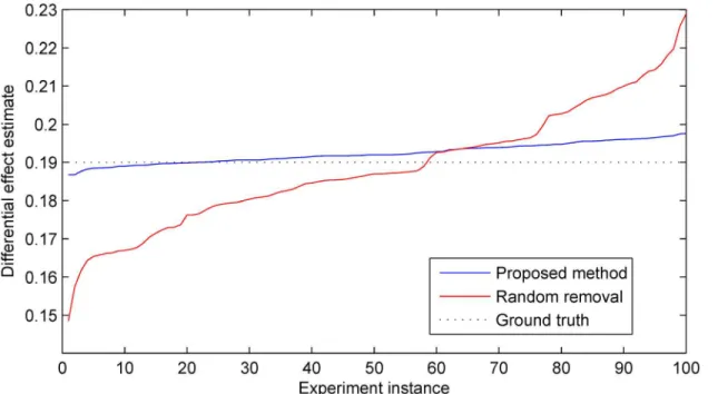
As expected, averaged over 100 instances of the simulated experiment there was no signifi-cant difference in the accuracy of the estimate of differential effects in the treatment group rela-tive to the control group between the two sample size reduction methods. In both cases the average accuracy was correct to within 1% with a statistically insignificant error from the ground truth. However an examination of the corresponding estimate precisions readily reveals a different picture. In particular across different experiment instances the proposed method results in approximately 70% lower standard deviation of the target estimate; this is illustrated inFig 4. This finding illustrates with clarity the argument we put forward in the preceding sec-tions. By performing sample selection in a manner which takes into account all available infor-mation, the statistically best decision can be made about which specific samples can be removed so as to ensure that in any particular case the associated information loss is mini-mized. In the experiments which follow, we sought to examine in detail how different parame-ters of a trial affect the precision improvement achieved with the proposed method.

Experiment 2: Effects of timing

As in the previous experiment, we used the data generation model fromExperimental setup

and compared the proposed method with random sample selection in the context of a single sample size reduction step. Our aim in this experiment was to investigate the effect that the timing of participant removal, that is, the cessation of the corresponding data accrual, has on the precision gained by using the proposed method. Hence we performed simulations for three

different time steps at which sample size reduction was performed,k= 30,50,70. All the other

parameters were kept constant—the number of participants removed was set ton= 50 (i.e.

approximately 28% of the total cohort size of 180), and the observability parameter which was

set toϕ= 0.01. As before the final outcomes were analysed afterkmax= 100 time steps using the

method described in [16], and for each combination of parameters 100 simulations were

performed.

(16)

selection-based approach—in both cases the average accuracy was correct to within 1% with a statistically insignificant error from the ground truth. On the other hand the difference in pre-cision was again stark and offered interesting insight into the proposed method. Our findings

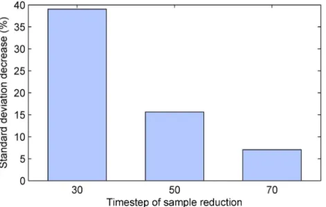
are summarized by the plot inFig 5which shows the reduction in the standard deviation of the

estimate of the differential effect of treatment, across different simulation instances. Firstly, observe that in all cases, that is, regardless of the time step at which sample size reduction was performed, the proposed method achieved superior results over the naïve alternative. Secondly, it is immediately apparent that the greatest benefit was found when sample size reduction was

performed earliest (i.e. afterk= 30 time steps). In this case the standard deviation of the

esti-mate was reduced extensively, by approxiesti-mately 39%. Lower but still substantial reduction of approximately 16% was achieved when sample removal was performed half-way though the duration of the simulated trials. When the removal was delayed to after 70% of the duration of the trial, the standard deviation reduction was still significant at approximately 7%.

The observed behaviour of our algorithm is unsurprising and could be readily predicted from theory.

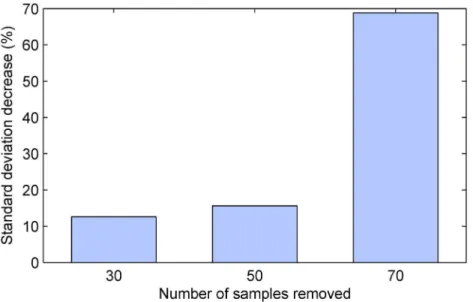
Experiment 3: Effects of size adjustment

In this experiment our aim was to investigate the effect that the magnitude of sample size reduction (i.e. the number of participants for whom data accrual is discontinued) has on the precision gained by using the proposed method. The experiment was set up in the same

man-ner asExperiment 2with the exception that now the time step at which sample size reduction

Fig 4. Estimates of the differential effect of treatment produced by the proposed method and the random selection-based baseline across 100 simulated trials.The estimates are shown ordered in magnitude for easier visualization. In all trial instances the reduction in the total number of participants ofn= 70 (i.e. approximately 39% of the total cohort size of 180) was performed afterk= 50 time steps. Following the removal time step, data accrual from the selected participants was discontinued but the data collected from them before that was still used in the final outcome analysis. Both the proposed method and the random selection-based baseline exhibited no bias, with a statistically insignificant error and the accuracy of within 1% from the ground truth. However the proposed method demonstrated far superior precision as readily observed from the plot; also see Figs5–7.

(17)

was performed was set tok= 50 and kept at this value in all simulation instances, while the number of participants who were removed from the continued accrual of data was treated as

an independent variable,n= 30, 50, 70. As before 100 simulations were performed with each

combination of parameters.

As in the previous experiments, the average accuracy of the estimate of the differential effects of the treatment intervention over control was the same regardless of the sample selec-tion strategy employed, but the corresponding precisions differed significantly. Our findings

are summarized by the plot inFig 6. Again, it is worth starting with the most obvious

observa-tion, which is that in all cases the proposed methodology resulted in an improvement. The greatest improvement was observed in the case when the sample size reduction was most dras-tic, with the proposed algorithm achieving nearly 70% lower standard deviation than the ran-dom selection-based alternative. This is of course consistent with our theoretical argument and

supportive of the propositions put forward in the preceding sections—the more the sample size

is reduced, the greater becomes the advantage of using all available information to make the adjustment targeted to the specific cohort.

Experiment 4: Effects of perceptibility

InBelief refinementwe highlighted the importance ofϕ, the observability parameter of the model used to generate trial data. Recall that this parameter was introduced to model the ease with which a participant can gauge the effects of the administered treatment i.e. the

partici-pant’s ability to observe an improvement or deterioration of the outcome of interest. The

sig-nificance that this inherent nature of the studied phenomenon has in the context of the proposed sample size reduction methodology can be readily appreciated by observing that the proposed approach derives key power from the stratification of patients based on their

responses to the auxiliary questionnaire (described inAuxiliary data collection). Consider the

Fig 5. The impact of sample size reduction timing on the precision of the estimate of the differential effect of treatment.Plotted is the decrease in the standard deviation of the estimate across different simulated trial instances (in %, relative to the random selection-based baseline). In all cases the proposed method demonstrates a substantial improvement over the baseline. Greatest improvement is achieved for early sample size adjustment. Also seeFig 4.

(18)

extreme case when perceptibility vanishes i.e. whenϕ= 0. In this case the collected auxiliary data is effectively random and as such contributes no useful information to guide the selection of participants which are to be removed from the trial. More generally, it can be said that the lower the perceptibility of the outcome, the less there is to be gained from using the proposed algorithm as compared to simple random selection.

Following the design adopted in the previous experiments, we performed 100 simulated tri-als for each combination of parameter values, while keeping all of the trial variables fixed

except for the observability parameter. In addition to the previously used value ofϕ= 0.01, we

examined the performance benefit of using our algorithm when observability was halved (ϕ=

0.005) and doubled (ϕ= 0.02). In all cases the number of removed participants was set to

n= 50 which was performed afterk= 50 time steps. The results are summarized inFig 7and

can be seen to match our theoretical expectations.

Experiment 5: Sequential adjustment

In the final experiment we report, we adopted a different experimental design than in the previ-ous experiments. Specifically, in the previprevi-ous experiments sample size reduction was under-stood to result in the cessation of data accrual for the removed trial participants, but the data accrued before their removal was still used in the final analysis of the trial outcomes. In con-trast, in this experiment all data for the removed participants, including the data accrued before removal, is discarded for the final analysis. This design captures those trial instances when the studied treatment exhibits cumulative effects which complicate the analysis of outcomes observed at different points in time.

Following the same practice as in the previous experiments, we used the data generation

model described inExperimental setup. However unlike before in this experiment sample size

Fig 6. The impact of sample size reduction magnitude on the precision of the estimate of the differential effect of treatment.Plotted is the decrease in the standard deviation of the estimate across different simulated trial instances (in %, relative to the random selection-based baseline). In all cases the proposed method demonstrates a substantial improvement over the baseline. Greatest improvement is achieved for the removal of a large number of participants. Also seeFig 4.

(19)

reduction was not performed at a single point in time. Rather a single participant was removed after each time step. Clearly this is not intended to replicate any realistic scenario which could be encountered in clinical practice. Though artificial in this sense, this experiment is useful as an analytical tool in the study of the behaviour of the proposed algorithm.

It is insightful to start with a look at the impact that the removal of a part of the cohort has on the estimate of the differential effect of the treatment intervention. A typical result is

illus-trated inFig 8. This plot shows the posterior distributions of the differential effect of the

treat-ment inferred after the removal of 120 individuals obtained using the proposed method (red line) and random selection (blue line). In both cases the posteriors were computed as described

in [16]. The most notable difference between the two distributions is in their spreads i.e. the

associated uncertainties. Specifically, the proposed method results in a much more peaked pos-terior, that is, a much more confident estimate. In comparison, the posterior obtained using random selection is much broader, admitting a lower degree of certainty associated with the corresponding estimate.

The accuracy of the two methods is better assessed by observing their behaviour over time.

The plot inFig 9shows themaximum a posterioriestimates of the differential effect of

treat-ment obtained using the two methods during the course of the trial. Also shown is the‘ground

truth’, that is, the actual differential effect which we can compute exactly from the setup of the

experiment (seeExperimental setup). In the early stages of the trial, while the magnitude of the

accumulated effect is small and the number of participants large, the two estimates are virtually indistinguishable, and they follow the ground truth plot closely. As expected, as the number of participants removed increases both estimates start to exhibit greater stochastic perturbations. However, both the accuracy (that is, the closeness to the ground truth) and the precision (that is, the magnitude of stochastic variability) of the proposed method can be seen to show

supe-rior performance—itsmaximum a posterioriestimate follows the ground truth more closely

Fig 7. The impact of outcome perceptibility on the precision of the estimate of the differential effect of treatment.Plotted is the decrease in the standard deviation of the estimate across different simulated trial instances (in %, relative to the random selection-based baseline). In all cases the proposed method demonstrates a substantial improvement over the baseline. Greatest improvement is achieved for trials with high outcome perceptibility. Also seeFig 4.

(20)

Fig 8. Posterior distributions of the differential effect of treatment after the removal of 120 participants i.e. after 120 time steps; see Eqs (32)–(42).

The method introduced in this paper results in a much more certain estimate of the differential, as witnessed by the highly peaked distribution, than does random selection.

doi:10.1371/journal.pone.0131524.g008

Fig 9. Themaximum a posterioriestimates of the differential effect of treatment during the course of the trial as an increasing number of

participants is removed.The blue line shows the estimates obtained using the proposed method, while the red line shows the estimates obtained using

random selection. Also shown is the‘ground truth’(green dotted line), that is, the actual differential effect computed exactly from the setup of the experiment (seeExperimental setup).

(21)

and fluctuates less than the estimate obtained when random selection is employed instead. It is also important to observe the rapid degradation of performance of the random selection method as the number of remaining participants becomes small, which is not seen in the

pro-posed method. This too can be expected from the theoretical argument put forward in

Sub-group selection—the statistically optimal choice of the sub-group from which participants are removed ensures that the posterior is not highly dependent on a small number of samples which would make it highly sensitive to the change in sample size.

Lastly, it is interesting to observe the differences between the changes in the sample sizes

within each sub-group using the two approaches. This is illustrated using the plots in Figs10

and11. As expected, when random participant removal is employed, the sizes of all sub-groups

decrease roughly linearly (save for stochastic variability), as shown inFig 10. In contrast, the

sub-group size changes effected by the proposed method show more complex structure,

gov-erned by the specific values of the belief and effect variables in our experiment, as shown inFig

11. It is particularly interesting to note that the size changes are not only non-linear, but also

non-monotonic. For example, the relative size of the control sub-group which includes

individ-uals which correctly identified their group assignment (i.e. the sub-groupGC−) begins to

increase notably after the removal of 30 participants and starts to decrease only after the removal of further 78 participants.

Summary and conclusions. In this paper we introduced a novel method for clinical trial adaptation. Our focus was on adaptation by amending sample size. In contrast to all previous

work in this area, the problem we considered was notwhensample size should be adjusted but

ratherwhichparticular individuals should be removed from the trial once the decision of

sam-ple reduction is made. Thus, our method is not an alternative to the current state-of-the-art,

Fig 10. The changes in the sample sizes within each of the six participant sub-groups (using the stratification described inMatching sub-groups

outcome modeland adopted from [16]) observed in our experiment using random selection based participant removal.Note the predictable outcome of the method, which results in a linear decrease of sample size for all sub-groups, and the contrasting behaviour of our approach inFig 11.

(22)

but rather a complementary element of the same framework. Our approach is based on the adopted stratification recently proposed for the analysis of trial outcomes in the presence of

imperfect blinding. This stratification is based on the trial participants’responses to a generic

auxiliary questionnaire that allows each participant to express belief concerning his/her inter-vention assignment (treatment or control). Extensive experiments on a simulated trial were used to illustrate the effectiveness of our method.

Acknowledgments

I would like to express my gratitude to Prof. Chiappelli and the anonymous reviewers whose many questions, comments, and suggestions greatly helped me identify the best manner to present the key contributions of my work.

Author Contributions

Conceived and designed the experiments: OA. Performed the experiments: OA. Analyzed the data: OA. Contributed reagents/materials/analysis tools: OA. Wrote the paper: OA.

References

1. Meinert CL. Clinical Trials: Design, Conduct, and Analysis. 3rd ed. New York, New York: Oxford Uni-versity Press; 1986.

2. Piantadosi S. Clinical Trials: A Methodologic Perspective. 3rd ed. Hoboken, New Jersey: Wiley; 1997.

3. Friedman L, Furberg C, DeMets D. Fundamentals of Clinical Trials. 3rd ed. New York, New York: Springer-Verlag; 1998.

Fig 11. The changes in the sample sizes within each of the six participant sub-groups (using the stratification described inMatching sub-groups

outcome modeland adopted from [16]) observed in our experiment using the proposed method.Compare withFig 10and note the data-specific behaviour of our approach.

(23)

4. Penston J. Large-scale randomised trials-a misguided approach to clinical research. Med Hypotheses. 2005; 64(3):651–657. doi:10.1016/j.mehy.2004.09.006PMID:15617882

5. Fisher LD. Self-designing clinical trials. Stat Med. 1998; 17:1551–1562. doi:10.1002/(SICI)1097-0258 (19980730)17:14%3C1551::AID-SIM868%3E3.0.CO;2-EPMID:9699229

6. U S Department of Health and Human Services. Guidance for Industry: Adaptive Design Clinical Trials for Drugs and Biologics. Food and Drug Administration Draft Guidance. 2010 Feb;.

7. Hung HMJ, Wang SJ, ONeill RT. Methodological issues with adaptation of clinical trial design. Pharma-ceut Statist. 2006; 5:99–107. doi:10.1002/pst.219

8. Orloff J, Douglas F, Pinheiro J, Levinson S, Branson M, Chaturvedi P, et al. The future of drug develop-ment: advancing clinical trial design. Nat Rev Drug Discov. 2009; 8(12):949–957. PMID:19816458

9. Berry DA. Adaptive clinical trials: the promise and the caution. J Clin Oncol. 2011; 29(6):606–609. doi: 10.1200/JCO.2010.32.2685PMID:21172875

10. Chow SC, Chan M. Adaptive Design Methods in Clinical Trials. Chapman & Hall; 2011.

11. Cui L, Hung HMJ, Wang SJ. Modification of sample size in group sequential clinical trials. Biometrics. 1999; 55:321–324.

12. Nissen SE. ADAPT: The Wrong Way to Stop a Clinical Trial. PLoS Clin Trials. 2006; 1(7):e35. doi:10. 1371/journal.pctr.0010035PMID:17111045

13. Lang T. Adaptive trial design: could we use this approach to improve clinical trials in the field of global health? Am J Trop Med Hyg. 2011; 85(6):967–970.

14. ArandjelovićO. Sample-targeted clinical trial adaptation. Proc Conf AAAI Artif Intell. 2015; 3:1693–

1699.

15. Arandjelović_{O. Assessing blinding in clinical trials. Adv Neural Inf Proc Sys. 2012; 25:530}_–_538.

16. ArandjelovićO. A new framework for interpreting the outcomes of imperfectly blinded controlled clinical trials. PLOS ONE. 2012; 7(12):e48984. doi:10.1371/journal.pone.0048984PMID:23236350

17. Haahr MT, Hróbjartsson A. Who is blinded in randomized clinical trials? A study of 200 trials and a sur-vey of authors. Clin Trials. 2006; 3(4):360–365. PMID:17060210

18. Berry SM, Carlin BP, Lee JJ, Müller P. Bayesian adaptive methods for clinical trials. CRC Press; 2010.

19. Kadane JB, editor. Bayesian methods and ethics in a clinical trial design. John Wiley & Sons; 2011.

20. Lawson AB. Bayesian disease mapping: hierarchical modeling in spatial epidemiology. CRC Press; 2013.

21. Oniško A, Druzdzel MJ. Impact of precision of Bayesian network parameters on accuracy of medical diagnostic systems. Artif Intell Med. 2013; 57(3):197–206. doi:10.1016/j.artmed.2013.01.004PMID: 23466438

22. Gelman A, Carlin JB, Stern HS, Rubin DB. Bayesian data analysis. Chapman & Hall/CRC; 2014.

23. Spiegelhalter DJ, Abrams KR, Myles JP. Bayesian approaches to clinical trials and health-care evalua-tion. John Wiley & Sons; 2004.

24. Berry DA. Bayesian clinical trials. Nat Rev Drug Discov. 2006; 5:27–36. doi:10.1038/nrd1927PMID: 16485344

25. Chen MH, Dey DK, Müller P, Sun D, Ye K. Bayesian clinical trials. In: Frontiers of Statistical Decision Making and Bayesian Analysis. Springer; 2010. p. 257–284.

26. Lee JJ, Chu CT. Bayesian clinical trials in action. Stat Med. 2012; 31(25):2955–2972. doi:10.1002/sim. 5404PMID:22711340

27. Berry DA. Adaptive clinical trials in oncology. Nat Rev Clin Oncol. 2012; 9(4):199–207. doi:10.1038/ nrclinonc.2011.165

28. Yin G. Clinical trial design: Bayesian and frequentist adaptive methods. John Wiley & Sons; 2013.

29. Broglio KR, Connor JT, Berry SM. Not too big, not too small: A Goldilocks approach to sample size selection. JJ Biopharm StatBiopharm Stat. 2014; 24(3):685–705. doi:10.1080/10543406.2014.888569

30. Gao P, Ware JH, Mehta C. Sample size re-estimation for adaptive sequential design in clinical trials. J Biopharm Stat. 2008; 18:1184–1196. doi:10.1080/10543400802369053PMID:18991116

31. Leon AC. Implications of clinical trial design on sample size requirements. Schizophr Bull. 2008; 34 (4):664–669. doi:10.1093/schbul/sbn035PMID:18469326

32. Zang Y, Lee JJ. Adaptive clinical trial designs in oncology. Chin Clin Oncol. 2014; 3(4):49.

(24)

34. James KE, Bloch DA, Lee KK, Kraemer HC, Fuller RK. An index for assessing blindness in a multi-cen-tre clinical trial: disulfiram for alcohol cessation-a VA cooperative study. Stat Med. 1996; 15(13):1421–

1434. doi:10.1002/(SICI)1097-0258(19960715)15:13%3C1421::AID-SIM266%3E3.0.CO;2-HPMID: 8841652

35. Bang H, Ni L, Davis CE. Assessment of blinding in clinical trials. Contemp Clin Trials. 2004; 25(2): 143–

156. doi:10.1016/j.cct.2003.10.016

36. Hróbjartsson A, Forfang E, Haahr MT, Als-Nielsen B, Brorson S. Blinded trials taken to the test: an anal-ysis of randomized clinical trials that report tests for the success of blinding. Int J Epidemiol. 2007; 36 (3):654–663. doi:10.1093/ije/dym020PMID:17440024

37. Kolahi J, Bang H, Park J. Towards a proposal for assessment of blinding success in clinical trials: up-to-date review. Community Dent Oral Epidemiol. 2009; 37(6):477–484. doi:10.1111/j.1600-0528.2009. 00494.xPMID:19758415

38. Sackett DL. Commentary: Measuring the success of blinding in RCTs: don’t, must, can’t or needn’t? Int J Epidemiol. 2007; 36(3):664–665. PMID:17675306

39. Hemilä H. Assessment of blinding may be inappropriate after the trial. Contemp Clin Trials. 2005; 26 (4):512–514. doi:10.1016/j.cct.2005.04.004PMID:15951244

40. Henneicke-von Zepelin HH. Letter to the Editor. Contemp Clin Trials. 2005; 26(4):512. doi:10.1016/j. cct.2005.04.004PMID:15936250

41. Wickens CD. Engineering Psychology and Human Performance. 2nd ed. New York: Harper Collins Publishers Inc.; 1992.

42. Berger V. Selection Bias and Covariate Imbalances in Randomized Clinical Trials. Hoboken, New Jer-sey: Wiley; 2005.

43. Biswas S, Liu DD, Lee JJ, Berry DA. Bayesian clinical trials at the University of Texas MD Anderson cancer center. Clin Trials. 2009; 6(3):205–216. doi:10.1177/1740774509104992PMID:19528130

44. Nelson NJ. Adaptive Clinical Trial Design: Has Its Time Come? JNCI J Natl Cancer Inst. 2010; 102 (16):1217–1218.

45. Meurer WJ, Lewis RJ, Tagle D, Fetters MD, Legocki L, Berry S, et al. An overview of the adaptive designs accelerating promising trials into treatments (ADAPT-IT) project. Ann Emerg Med. 2012; 60 (4):451–457. doi:10.1016/j.annemergmed.2012.01.020PMID:22424650

46. Kullback RA, Leibler S. On Information and Sufficiency. Ann Math Stat. 1951; 22(1):79–86. doi:10. 1214/aoms/1177729694

47. Bhattacharyya A. On a measure of divergence between two statistical populations defined by their probability distributions. Bull Calcutta Math Soc. 1943; 35:99–109.

48. Hellinger E. Neue Begründung der Theorie quadratischer Formen von unendlichvielen Veränderlichen. J Reine Angew Math. 1909; 136:210–271.

49. Gilks WR. Markov Chain Monte Carlo in Practice. 1st ed. Chapman and Hall/CRC; 1995.

50. Aitchison J, Brown JAC. The Lognormal Distribution. Cambridge University Press; 1957.

51. Ly LP, Jimenez M, Zhuang TN, Celermajer DS, Conway AJ, Handelsman DJ. A double-blind, placebo-controlled, randomized clinical trial of transdermal dihydrotestosterone gel on muscular strength, mobil-ity, and quality of life in older men with partial androgen deficiency. J Clin Endocrinol Metab. 2001; 86 (9):4078–4088. doi:10.1210/jcem.86.9.7821PMID:11549629