Asynnnetric smiles, leverage effects and structural parameters

' " #"FUNDAÇÃO . ' " GE1UUO VARGAS

<..;;\·i\lIN \RI()S DI \lI S<)t 1I <..;; \ !·("ON()i\lIC \

..

EPGE ＭｾＭｾＭＭ

Escola de Pós-Gtaduaçao em Economia

•

"Asymmetric Smiles,

Leverage Effects and

Structural Parameters"

Prof. René Garcia

(Université de Montréal, CIRANO E CRDE)

LOCAL

Fundação Getulio Vargas

Praia de Botafogo, 190 - 10° andar - Auditório- Eugênio Gudin

DATA 27/0712000 (5a _feira)

Asynnnetric Smiles, Leverage Effects and

Structural Parameters

Renê Garcia

Université de Montréal, C/RANO and CRDE

Richard Luger

Bank of Canada and C/RANO

Éric Renault

Université de Montréal, C/RANO, CRDE, and CREST-/nsee

First version: June 1999 This version: July 2000

Keywords: Equilibrium Option Pricing, Recursive Utility, Black-Scholes

Im-plicit Volatility, Smile effect. JEL Classification: C1,C5,G1

Address for correspondence: Départment de Sciences Économiques et C.R.D.E., Université de Montréal. C.P. 6128. Succ. Centre-Ville, Montréal, Québec, H3C 3J7, Canada.

1. Introduction

In the empirical option pricing literature, departures from the Black-Scholes (1973)

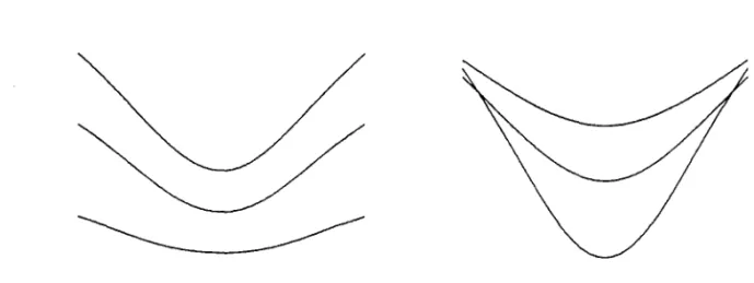
(BS) model are often characterized by an implied volatility curve, whereby the volatility extracted from the BS option pricing formula given the observed option price is graphed against the moneyness of the option. The empirical biases of the BS model have been dubbed the smile effect in reference to a symmetric implied volatility curve, but numerous distorted smiles in the shape of smirks or frowns

are inferred more frequently from market data. In Figure 1, we graphed several

volatility curves for options on the S&P 500 index on selected dates to reflect the types of shapes that can be observed most frequently. A stochastic volatility model as in Hull and White (1987) produces a symmetric smile when the returns innovations and the volatility are uncorrelated. With stochastic volatility, the price of the option is expressed as an expectation of the BS price, where the ex-pectation is taken with respect to the distribution of the heterogeneous stochastic volatility factor. The symmetric volatility smile is created by a related Jensen effect (see Renault, 1997 and Renault and Touzi, 1996).

Asymmetric smiles can therefore be potentially explained by an instantaneous correlation between returns and volatility. In Black (1976), an inverse relationship between the leveI of equity prices and the instantaneous conditional volatility is put forward for individual firms. This inverse relationship is explained by financiai leverage. A drop in the price of the stock increases the debt-to-equity ratio and therefore the risk of the firm, which translates into a higher volatility of the stock. Nelson (1991) shows also that such a negative correlation exists for broad market indices. The correlation is still called a leverage effect, but explanations are given in terms of time-varying risk premia and volatility feedback (see Campbell and HentscheL 1996, among others). Ifvolatility risk is priced, an anticipated increase in volatility raises the discount rate of future expected dividends and lowers the

present equity price1 . From a theoretical perspective, Platen and Schweizer (1998)

1 Based on portfolios constructed from l\'ikkei 225 stocks, Bekaert and Wu (2000) find support

explain the asymmetric shape of the smile by developing a model in which the diffusion process of the stock price incorporates the technical demand induced by

hedging strategies2_{• David and Veronesi (1999) propose an incomplete information}

mo dei where investors' uncertainty explains the intertemporal variation in the slope and curvature of implied volatility curves.

In this paper, we characterize the asymmetries of the smile through multiple

leverage effects in a stochastic dynamic asset pricing framework. The dependence between price movements and future volatility is introduced through a set of latent state variables. These latent variables can capture not only the volatility risk and the interest rate risk which potentially affect option prices, but also any kind of correlation risk and jump risk. The standard financial leverage effect is produced by a cross-correlation effect between the state variables which enter into the stochastic volatility process of the stock price and the stock price process itself. However, we provide a more general framework where asymmetric implied volatility curves result from any source of instantaneous correlation between the state variables and, either the return on the stock or the stochastic discount factor.

To be able to put forward the asymmetric deformations of the smile, we first state necessary and sufficient conditions for symmetry in a general setting. These characterizations are given in terms of the option pricing function or, alterna-tively, through the skewness of the pricing probability measure. We capture the aforementionned skewness of the pricing probability measure through a general-ized option pricing formula based on a stochastic discount factor containing state variables. As special cases of our formula we obtain of course the BS formula, but also the Hull and White (1987) and Bailey and Stulz (1989) stochastic volatility option pricing formulas and the Merton (1973), Thrnbull and Milne (1991), and Amin and Jarro\\' (1992) stochastic interest rate option pricing formulas for equity options.

This extended option pricing formula is motivated by the vast

empiricallitera-for volatility feedback effects.

2Grossman and Zhou (1996) propose also an equilibrium model of risk sharing between portfolio insurers and investors which generates a negatively skewed smile. In Renault (1997), a very small discrepancy between the option markets assessment of the stock price and the actual price can capture sensible asymmetries of the smile.

ture aimed at finding option pricing mo deIs that wiU reproduce the cross-sectional patterns and the dynamics. of implied volatilities. A class of generalized determin-istic volatility models has been proposed to overcome the empirical biases of the

BS model3 . In this class of models, the local volatility of the underlying asset is

a known function of time and of the path and leveI of the underlying asset price. However, Dumas, Fleming and Whaley (1998) show clearly that deterministic volatility models overfit the smile in sample and loose any predictive power out of sample. Buraschi and Jackwerth (1997) bring further evidence that deterministic volatility models are not consistent with observed option prices and that stochas-tic volatility mo deIs are more likely to explain the smile. Other evidence against the one-dimensional diffusion mo deI can be found in Bakshi, Cao, Chen (1999). They show that call prices often go down when the underlying price goes up and that call prices are not perfectly correlated with each other and the underlying asset.

The main stochastic volatility mo deIs that have been submitted to empirical testing are variants of the two-dimensional (stock returns and volatility) diffusion model. Although these mo deIs produce patterns qualitatively similar to some violations, quantitatively, they only bring marginal improvement to the fit of option-price changes. Bakshi, Cao and Chen (1997), Bates (1996) and Chernov and Ghysels (1999) provide evidence against the stochastic volatility mo deI of Heston (1993). Multi-factor volatility mo deIs as in Bates (1997) and Gallant, Hsu, Tauchen (1998) do not bring a significant improvement. The main conclusion is that an extremely high volatility of volatility is necessary to generate leptokurtosis of the magnitude consistent with the volatility smirks. Das and Sundaram (1999) explain that stochastic volatility mo deIs are not capable of generating high leveIs of skewness and kurtosis at short maturities under reasonable parameterizations. Jump-diffusion mo deIs can generate realistic implied volatility smiles at short maturities (see Bates. 1997, Bakshi, Cao and Chen, 1997, Andersen, Benzoni and Lund. 1998). Das and Sundaram (1999) show that, consistent with empirical

lO

patterns, the degree of skewness and excess kurtosis declines as maturity increases in a jump-diffusion model, but that for reasonable values of the parameters the decline is far more rapid than would be suggested by the data. Therefore, jump-diffusion models cannot reproduce the implied volatility smile at long horizons since it flattens out too quickly. Pan (1999) examines joint time series data on spot and option prices on the S&P 500 and provides evidence of a jump risk premi um that responds quickly to market volatility and is important in explaining the volatility smirks. There remains however some misspecifications and some suggestions regarding the inclusion of jumps in the volatility are made.

The conclusion of this empirical literature is that important features for re-producing the cross-sectional patterns and the dynamics of implied volatilities are jumps in the returns, correlation between jumps and volatility, and jumps in volatility. To illustrate how our option pricing formula can incorporate these features, we specialize our latent state variables to a discrete-state Markov pro-cesso A discrete change of state will affect simultaneously the mean and variance of equity returns and of the stochastic discount factor, creating jump-like effects also in volatility. In this setting we characterize analytically both the skewness of the returns and the equity leverage effect. We show that the formulas for condi-tional skewness and leverage effect in the stock are very similar. We establish the conditions for negative skewness or leverage in terms of transition probabilities between states.

To be able to draw the shapes of the implied volatility smiles, we need to further specify the stochastic discount factor. We choose an an example an equilibrium-based stochastic discount factor in the spirit of Rubinstein (1976), Brennan (1979) and Amin and Ng (1993). We set our equilibrium mo deI in a recursive utility framework with time non-separable preferences (Epstein and Zin [1989])-1. Our latent variable framework makes it possible to parameterize

parsi-4Two papers have used preferences that disentangle risk aversion from intertemporal substi-tution in the context of option pricing. Detemple (1990) uses the ordinal certainty equivalence hypothesis proposed by Selden (1978) in a two-period economy and shows that time preferences play a distinctive and significant role in pricing options. For example, option prices change with the expected return on the stock and may decrease when the risk of the stock return increases. Ma (1993) extends the stochastic differential utility concept in Duffie and Epstein (1992) to a mixed Poisson-Brownian information structure and derives a closed-form pricing formula for

moniously the dynamic evolution of the consumption and dividend processes in this equilibrium mo deI. We use a two-state bivariate Markov switching model as

in Cecchetti, Lam and Mark (1993) and Bonomo and Garcia (1993, 1996)5.

When we calibrate this model to reasonable values of the parameters, we are able to reproduce the various types of implied volatility curves inferred from option market data. In other words, not only our mo deI reproduces asymmetric smiles but it allows for reversals in the smile skewness. AlI the classic extensions of the basic Black-Scholes model with stochastic volatility, stochastic interest rates or

jumps reviewed in Bakshi, Cao and Chen (1997) cannot produce such reversals.

Indeed, as Bates (1996) emphasized, it is such changing skewness in the smile

that poses a challenge to current option pricing models. In our setting, reversals in skewness can occur when the source of risk changes.

The rest of the paper is organized as follows. Section 2 provides general con-ditions under which the smile is symmetric. Section 3 develops a generalized option pricing formula with latent state variables. Based on this formula, Section 3 shows that the asymmetric distorsions of the smile are due to leverage effects. A comparison with usual stochastic volatility mo deIs with leverage is developed in Section 5 as well as an analytical characterization of Ieverage when state variables follow a discrete-state Markov processo Section 6 provides a simulation exercise using an equilibrium-based stochastic discount factor in order to illustrate the various shapes of the smile that the mo deI can produce. Section 7 concludes and announces further empirical assessment of the proposed option pricing model.

2. The symmetry af the valatility smile

To characterize the asymmetry of the impIied volatility curves, one needs a bench-mark model which will produce a symmetric curve. When the volatility is

stochas-tic as in the Hull and White (1987) model, Renault (1997) and RenauIt and

Touzi (1996) have shown that the shape of the volatility structure with respect

European cal! options written on aggregate equity under Kreps-Porteus preferences.

•

•

to the moneyness of the option is symmetric when the returns innovations and

the volatility are uncorrelated. Moneyness Xt is defined as the logarithm of the

ratio of the forward price

ｾｶ･ｲ＠

the strike price, Xt = Log K

ｂｾ［Ｌ＠

T) (with St the

price of the underlying asset, K the strike price and B(t, T) the price of apure

discount bond maturing at T). Since both the BS and the Hull and White option pricing formulas are homogeneous functions of degree one with respect to the pair

(St, K), we wiIl provide new characterizations of the symmetry of the volatility

smile in the context of a general homogeneous option pricing formula, both in terms of the option pricing function and of the pricing probability measure .

The theory for pricing contingent claims in the absence of arbitrage introduces

a pricing probability measure Qt,T under which the price llt at time t of any

contingent claim maturing at time T is the discounted expectation of its terminal payoff. In the case of a European call option with strike price K, it is given by:

llt = B(t, T)E;(ST - K)+, (2.1)

where E; denotes the expectation operator with respect to Qt,T 6. We will

there-fore compare a general but homogeneous option pricing formula llt(St, K) as

de-fined in (2.1) with the BS option pricing formula dede-fined itself by a homogeneous

function BS(.,., a), for a given volatility parameter a, with:

{

BS(St,K,a)

=

St<p(dl ) - KB(t,T)<p(d2 ),

d,

ｾ＠ ｬｲＭＺｾ､ｘｴ＠

_{a T- t}

+

!".2(T ₂ - t

l] ,

d2 = dI - a T - t.

(2.2)

The BS implied volatility is defined as a function ｡ｾＨｸ､＠ of the moneyness Xt

only, and not of St and K separately:

(2.3)

since a direct application ofthe homogeneity of degree one ofIIt(.,.) and BS(.,., a)

with respect to the pair (St, K) allows one to divide each side of (2.3) by St and

6Existence and unicity of Qt.T were studied by several authors since the seminal pape r of Harrison and Kreps (1979). In this paper. we are only interested in the existence of a pricing probability measure Qt.T which is well-defined and given to us, whether it is uni que or noto

•

conclude that

0";

(Xt) is well-defined as a function of K / St or (equivalently) of Xt

by:

(2.4)

with the obvious change of notation.

In this setting, we can investigate the slope of the BS implied volatility

0";

(x)

as a function of its distance x to the money, remembering that moneyness x is

equal to O at the money, that is when the strike price coincides with the forward

price ｂＨｾＺｔＩＧ＠ In particular, two strike prices KI and K2 are said syrrunetric with

respect to the money if the corresponding Xl and x2 are symmetric with respect

to zero, since in this case KI and K2 are on each side of the forward price but

their geometric average coincides with the forward price. Therefore, the relevant symmetry property of the volatility smile is the following:

O";(x) =

0";(

-x) for any x. (2.5)

In Proposition 2.1 below, we extend a ｾ･ｳｵｬｴ＠ first stated in Renault and Touzi

(1996), which characterizes the symmetry of the smile in terms of the option

pricing function 7 .

Proposition 2.1. lf option prices are conformable to a homogeneous option

pric-ing formula x -. 7r(x), the volatility smile is symmetric (O"*(x)

=

O"*(-x) for any

x ) if and only if for any x:

Proof: See Appendix l.

This characterization of the symmetry of the smile admits an equivalent for-mulation in terms of the pricing probability measure. While the pricing probabil-ity measure is usually characterized through the cumulative distribution

func-tion of

i:,

it is convenient here to characterize it through either the

cumu-lative distribution function _FVT (.) or the probability density function fVT (.) of

•

TT _ L STB(t, T) ( )

VT - og S . We are then able to prove see Appendix 1 the following

. . t

proposltlon:

Proposition 2.2.

lf

the cumulative distribution function FVT (') of VT under a

pricing probability measure is absolutely continuous (associated with a density

function fVT (.) = ｆｾｔ＠ (.)) and such that exp(VT ) is integrable, the volatility smile is

symmetric if and only if one of the following three equivalent properties is fulfilled:

(i) For any x:

(ii) For any x:

(iii) There exists an even function g(.) such that for any x:

These characterizations offer various ways to extend the BS formula, while keeping both a homogeneous option pricing function and a symmetric smile. Characteri-zation (i) provides a theoretical support to descriptive approaches which replace the standard normal cumulative distribution function of the BS formula by alter-native distribution functions, possibly asymmetric. It shows that in order to keep a symmetric smile, the term 1-FVT (-x) should replace FVT (x) in the second part of the option pricing formula. Characterization (ii) should be interpreted in terms of hedging. lndeed, Garcia and Renault (1998) have shown that E;[eVT l[VT2:-xJl

is precisely the hedging ratio, in other words the derivative of the option pricing function with respect to the stock price (the so-called delta of the option)8. Fi-nally, for characterization (iii), it should be noticed that if the pricing probability

IITheir proposition 2.1 shows that this characterization of the hedging ratio is a necessary and sufficient condition for homogeneous option pricing. Since hedging is not the primary focus of this paper, we leave to the reader the interpretation of this fairly natural relationship between F V_T (x) and the delta coefficient.

measure is characterized by a conditionallog-normal distribution of future returns

given available information at time t :

STB(t, T)

I

N( 2

VT = Log St It -(Qt,T) J..Lt,CTt ),

the condition of Proposition 2.2 means that :

which is automatically fulfilled in the absence of arbitrage since, by application

of (2.1) with K = O, we have:

St = B(t, T)E; ST.

In the next subsection, we provi de sufficient conditions on the pricing prob-ability measure to ensure the homogeneity of the option pricing function in a convenient stochastic framework with state variables.

3. A generalized Black-Scholes and Hull-White formula with state vari-ables

Merton (1973) stressed that the desirable homogeneity of option prices will be

maintained as soon as asset returns are serially independent. This condition

ex-pressed in terms of the data generating process (DGP) of the underlying asset can be slightly generalized by expressing it in terms of the pricing probability measure. Given the general option pricing formula (2.1), the required homogene-ity property amounts to the following conditional independence property (with respect to Qt,T )910 :

9This condition for homogeneity is more general than the sufficient condition proposed by Merton (19i3) since it is stated in terms of the pricing probability measure rather than the DGP. lndeed. we do not preclude a possible dependence of the risk premiums on the stock price St, which could violate assumption 3.1 for the DGP. Garcia and Renault (1998) offer a precise characterization of this property in the standard setting of continuous time arbitrage pricing.

11

(3.1)

A way to generalize the BS and HW formulas while keeping the functional shape

of the BS formula is to recover log-normality conditionally to the full path of a

vectorial process (Ut)tEN of possibly unobserved state variables. Indeed, while the

BS geometric Brownian motion world is obviously unrealistic due to heterogeneity factors, it is much more general to assume that log-normality is recovered after conditioning on a number of state variables. In particular, it is a standard way to

capture the leptokurtic feature of financial time seriesll .

3.1. A State-Variable Framework for Homogeneous Option Pricing

State variables have two basic distinctive features: they are exogenous and they

summarize the dynamics ofthe variables ofinterest (see Renault (1998) and Garcia

and Renault (1999) for a general discussion). We provide below a definition in

the context of a pricing probability measure Qt,T, t = 1, ... , T without specifying

its dynamics at this stage .

Definition 3.1. : A vectorial process (Ud ｬｾｴｾｔ＠ (also written U'[) is called a state

variable process12 _{with respect to the stock price process Ｈｓｴｨｾｴｾｔ＠ and the family} of pricing probability measures (Qt,T )l$t:5T if for any t

=

1, ... , T -1, the Qt,T joint probability distribution ｯｦＨｾＬ＠ Ur , T

>

t) does not depend on the past ofthe price process (Sr ｨｾｲｾｴＮ＠

llSince Clark (1973), there is a long tradition ofthis approach in financiai econometrics. Clark (1973) stressed that non-normality is a puzzle when one has in mind the geometric temporal averaging of the returns and a corresponding centrallimit theorem argumento In this respect, log normality of returns can be invoked without any significant loss of generality once it is recovered after conditioning on a sufficient number of state variables. As far as option pricing is concerned, the role of heterogeneity factors has been enhanced by Renault (1997) in a general setting which encompasses in particular Merton (1976) jump-diffusion model and Hull and White (1987) stochastic volatility mode!.

12In many applications of the state variable concept. Markovianity is usually postulated. Then, the relevant conditioning information is summarized by a few recent lags of the state variable processo Since this Markovianity assumption is not needed at this stage, we maintain in full generality the whole past U[ of this processo

This definition implicitly means that Qt,T is a family of transition probabilities

indexed by a conditioning set It which includes the joint past (Sn UT ｨｾｔｾｴ＠ of

prices and state variables. By writing the usual factorization of probability density functions:

(3.2)

the above definition means that the state variable process Ut is exogenous in

the sense of being independent of the past of the price process conditionally to its own past and that the future returns are conditionally independent of past returns given the full path of state variables which, in this sense, summarize the dynamics of the price processo To make this point clear, in the particular case where the available information at time t is described by the sigma field:

(3.3)

the factorization (3.2) can be rewritten as follows, given the state variable concept just described above:

(3.4)

It is then clear in this context that (3.4) is a sufficient condition for the

homo-geneity property (3.1).

The symmetric smile condition of Proposition 2.2 is also valid in the more

general setting just described. If VT follows under Qt,T a conditional Gaussian

distribution N[l-Lt(Un. O"z(Unl given lt and the path Ur (between t and T) of

some state variables U, the symmetry condition will be fulfilled (by integration

over Ur) as soon as:

probability measure is required for the symmetry of the smile. In particular, it

shows that it is not the density of the log returns that should be symmetric (as it

is commonly believed perhaps because of the usual log-normal setting), but the same density rescaled by a suitable exponential function.

3.2. An Option Pricing Formula with a General Stochastic Discount Factor

In order to generalize the Hull and White model, we will assume from now on

that the pricing probability measure Qt,T is defined through a stochastic discount

factor (SDF) mt,T :

(3.5)

where Et denotes now the conditional expectation operator with respect to the

DGP. Hansen and Richard (1987) provide some general conditions under which

the existence and positivity of mt,T is guaranteed. First, to ensure homogeneity

of the option pricing formula, we will make two sufficient assumptions about the joint dynamics of the stochastic discount factor, the stock returns and the state variables.

Assumption A: The SDF mt,T can be factorized as follows:

T-1

mt,T = ).,t,T(U[)

rr

mr+1, (3.6)

r=t

where it is assumed that:

AI: The process (mr+1' ｓｾｾｬ＠ h::;r::;T-1 does not cause the process (Ur L:S;T:S;T;

A2: The variables (mr+1' _{ｓｾ［ｬ＠} h::;r::;T-1 are serially independent given

Ur

The conditions (AI) and (A2) are consistent with the concept of state variables

introduced in Definition 3.113 . The non-causality property may be interpreted

equivalently in Granger (1969) or in Sims (1972) terms. Granger causality means

that, given the past

Ui

of state variables, the past observation of processes mr

and Sr does not bring any relevant information to forecast Ut+1 (which is in

13See Garcia and Renault (1999) for a detailed account of this point under both the pricing probability measure and the DGP.

this sense exogenous). Sims causality means that the probability distribution of (mt+l, ｓｾＭ［ｬＩ＠ given It and Ur+l does not depend upon Ur+-l' Jointly with the

conditional independence assumption A2, assumption AI permits to characterize

the joint probability distribution of (mT+l' ｓｾ［ｬＬ＠ UT+l)T?t given It as the following

product:

Proposition 3.2. : Under (Al) and (A2) there exists a deterministic function

Wt,T such that the option price (3.5) can be written as:

7ft = Wt,T

[Ui,

ｾ｝＠

St·

Proposition 3.2 establishes that the option pricing formula is homogeneous of

degree one with respect to the pair (St, K).

To obtain a generalized BS and Hull-White option pricing formula starting

from (3.5), one needs only, in addition to the previous assumptions (AI) and (A2),

a joint log-normality assumption of mt,T and ｾ＠ given It

=

CT[mT,ST' UT, T ｾ＠

t]

and a path Ur+-l of state variables.

Assumption A3: The conditional probability distribution of (log mt+l,log ｓｾｾｉＩ＠

. Ut_{+1 ' c t-l T 1 b' . t 1·}

glven 1 lS. lor - , ... , - ,a lvarla e norma.

Proposition 3.3. Under assumptions Al, A2 and A3:

(3.8)

and:

-2

O't,T

ｾ＠

at,T _1 L

[Q

(

T)B(t,T)]

- _ +

+ _

09 ms t, ＭＺ｟ｾＭＭＧＭ

O't,T 2 O't,T B(t, T)

- d1(x) -at,T

T-l

- LO';r+l'

r=t

T-l T-l

- T """' 1 """' 2

B(t, T) = Àt,T(U1 ) ･ｸｰＨｾ＠ J-lmr+l

+

"2

ｾ＠ O' mr+l),

r=t r=t

(3.9)

To put this general option pricing formula in perspective, we will compare it to pricing formulas based on equilibrium or on the absence of arbitrage. Con-cerning the equilibrium approach, our setting is very general since it is based on a stochastic model for the SDF which does not rely on restrictive assumptions about preferences, endowments, or agent heterogeneity. Moreover, our factorization for the SDF is more general than the usual one mt _, T = !Lz:_TI, 1

4,

with the standard interpretation as an intertemporal marginal rate of substitution. Actually, the additional factor Àt,T(U'{) in our SDF allows to accommodate non-separable or

state-dependent preferences. The non-separable case will be illustrated in the last section by a recursive utility setting. An example of state-dependent preferences could be habit formation based on state variables.

Of course. the benchmark option pricing formulas are based on the absence of arbitrage.Our general formula (3.8) nests a large number of preference-free extensions of the Black-Scholes formula. In particular if Qms(t, T)

=

1 and

B

(t, T)

=

ｉｬ［ｾｴｬ＠ B ( T. T

+

1) ,one can see that the option price (3.8) is nothing but the conditional expectation of the Black-Scholes price, where the expectation is computed with respect to the joint probability distribution of the rolling-over

l-lSee for instance Amin and Ng (1993b) and Bollerslev and Mikkelsen (1996) following Con-stantinides (1992) and Turnbull and Milne (1991).

interest rate rt,T = - ｌＺ［ｾｴｬ＠ log B ( T, T

+

1) and the cumulated volatility at,T' This

framework nests three well-known models. First, the most basic ones, the Black and Scholes (1973) and Merton (1973) formulas, when interest rates and volatil-ity are deterministic. Second, the Hull and White (1987) stochastic volatilvolatil-ity

extension, since a;,T =

Var

[log

ｾ＠

I

U[]

corresponds to the integrated volatility

Jt

ｏＧｾ､ｵ＠ in the Hull and White continuous-time setting. Third, the formula al-lows for stochastic interest rates as in Thrnbull and Milne (1991) and Amin and Jarrow (1992). However, the usefulness of our general formula (3.8) comes above alI from the fact that it offers an explicit characterization of instances where the preference-free paradigm cannot be maintained. Usually, preference-free option pricing is underpinned by the absence of arbitrage in a complete market setting. However, our SDF-based option pricing does not prec1ude incompleteness and points out in which cases this incompleteness will invalidate the preference-free paradigm. The only cases of incompleteness which matter in this respect occur precisely when at least one of the two following conditions:

(3.10)

T-l

B(t, T)

=

rr

B(T, T

+

1) (3.11) T=t

is not fulfilled.

In general, preference parameters appear explicitly in the option pricing

for-mula through B(t, T) and Qms(t, T) since these two quantities depend on the

characteristics of the SDF: Àt,T(U[), (ILmT+l' 0'2 mT+l,O'msT+l)i=t1. However, in

B(t,t+1)=Et [B(t,t+1)] - (3.12) as shown in Appendix 2. Therefore, observing the bond price will make preference

parameters in B (t, t

+

1) vanish from the option price as soon as B (t, t

+

1) =

B(t, t

+

l),that is if and only if B(t, t

+

1) belongs to the information set

ft.

A useful way of writing the stock pricing formula is:

Et [Qms(t, t

+

1)] = 1, (3.13)

Therefore, similarly to the bond pricing, the stock pricing will make preference

parameters vanish from the option price, as soon as Qms(t, t+ 1) is known at time

t and therefore equal to one. From (3.9), we can then express the conditional

expected stock return as:

E [Sst+tlIIt] _ _{B(t, t} 1

₊

_{1) exp} [ _{-amst+l ,} ]

which is very dose to a standard conditional CAPM equation. Therefore, the

fact that both B(t, t

+

1) and Qms(t, t

+

1) are known at time t produces both a

preference-free option pricing formula and a CAPM-like stock pricing equation15 . To condude, it should be stressed that even in an equilibrium framework with incomplete markets, option pricing is preference-free if and only if there is a kind

of predictability property ( B(t, t

+

1) and Qms(t, t

+

1) are known at time t)

according to the terminology introduced by Amin and Ng (1993a)16. We will now show that the lack of such predictability corresponds in a general sense to a leverage effect.

4. The asymmetric distortions of the smile due to leverage effects

In this section, we focus on the option pricing formula provided by Proposition (3.3) to characterize the cases where the corresponding volatility smiles are

sym-I" A similar parallel is drawn in an unconditional two-period framework in Breeden and Litzen-berger (1978).

160ur characterization of preference free option pricing by a predictability property generalizes the one provided by Amin and Ng (1993a) since it does not depend upon a particular equilibrium setting with specific preferences and endowments.

..

metric. According to criterion i) of Proposition (2.2) for the symmetry of the smile, it means that the above option pricing formula:

can be written:

But it can be seen in the derivation of the option pricing formula (3.8) (see Appendix 2) that:

(4.1)

Therefore, a necessary and sufficient condition for symmetric smiles of (3.8) is that:

or equivalently:

Ed

Q=(t, T)<I>(d, (x))}

ｾ＠

1 - E, {

ｾｩＺＺ＠ ｾ［＠

<I> (d,( -x)) } (4.2)

But from (3.8):

d2(-x) = -d1(x)

+

.l:-Log [Qms(t,T)B(t,T)].

at,T B(t, T)

Thus by taking into account that

ｅｴｦＡｩｾＺｾｬｊ＠

= 1, the symmetry criterion can be rewritten:

We have therefore proven the following proposition:

..

EdQms(t,T)cp(d1(x))} = Et B( T) { B(t, T) _t, cp(d1(x) - =-Log _(jt,T 2 [ Qms(t,T) B(t, T)] _{B(t, T)} ) }

A sufficient condition for a symmetric volatility smile is:

that is:

B(t, T) Qms(t, T)

=

B(t, T)'

S

[ T - l ]

E[;:

IU[]

=

ｂＨｴｾ＠

T)

Et[exp[-

ｾ＠

(jmsr+llJ

(4.3)

(4.4)

(4.5)

It should be stressed that the sufficient condition (4.4) is always fulfilled in expectation because, as shown in Appendix 2, the bond and stock pricing formulae are respectively given by:

B(t, T) = Et [B(t, T)] , and (4.6)

Et [Qms(t, T)]

=

1. (4.7)

ｾｶｉｯｲ･ｯｶ･ｲＬ＠ taking into account the highly nonlinear features of the two sides

of the necessary and sufficient identity (4.3), Jensen effects are likely to violate it if (4.4) is not fulfilled. In other words, condition (4.6) (or equivalently (4.7)) appears at first sight not too far from being necessary.

In terms of expectations with respect to the available information lt at time t, a consequence of condition (4.7) is a CAPM-type pricing equation:

S,

ｾ＠

B(t,

T)E, [E[ST1U[j

･ｸｐ｛ｾ＠

<7m

'Hd]

(4.8)

This is something like a martingale restriction (see Longstaff, ) on the stock price at time t which, if violated, is likely to introduce skewness in the volatil-ity smile. In the particular setting of an Hull and White model, Renault (1997)

provides simulation evidence to show that a very small discrepancy (as low for

ex-ample as 0.1 per cent) between the stock price St and its model-based theoretical

value may induce severe skewness in the smile. In order ot interpret this

restric-tion, one may notice that the general stock pricing equation (4.7) only implies that:

S, = E,

[B(t,

T)E[STIU[]

･ｸｰ｛ｾ＠

<Tmff+I[]

(4.9)

In other words, by taking into account the bond pricing equation (4.6), the

asymmetries of volatility smiles that we capture here are produced by a nonzero conditional covariance:

Cov,

[B(

t,

T), E[STIU[]

･ｸｐ｛ｾ＠

<Tmff+IJ]

;<

O. (4.10)

This covariance represents a first channel through which the various leverage effects described in subsection 2.4 above result in asymmetric distorsions of the volatility smile. This channel is basically a correlation between the interest rate

risk and the stock risk, measured as idiosyncratic risk as well as market risk. 17 Of

course, another source at the origin of the asymmetric distorsions of the volatility

smile stems from alI the random features (given It) of Qms(t, T) which are not

summarized by the interest rate risk in B(t, T). Typically, according to (3.9),

the cause is the lack of predictability at time t of ｅ｛ｾＯｕｔｬ＠ and ｌＺｾｾｴＱ＠ (}msr+1.

However, it should be remembered that, as long as the SDF can be factorized as in the classical case of time-separable preferences (mt _, T

=

'!lI.), _'1t we have:

T-1

Qms(t, T) =

TI

Qms(r, r

+

1), (4.11)

r=t and then:

..

Q

ms (t, T)

=

1 if

Q

ｾｳ＠ ( r, r

+

1)

=

1 for r

=

t, t

+

1, ... , T - 1. (4.12)

In other words, only leverage effects at the stock price leveI (for both idiosyn-cratic and market risk) can produce in this case asymmetric volatility smiles.

5. A Comparison with Stochastic Volatility Models with Leverage

The predictability property referred to in the previous sections amounts to the knowledge at time t of the quantities

B

(t, t

+

1) and Qms (t, t

+

1) which can be

written as:

B

(t, t

+

1) - Àt,t+l (U:+1) Et [mt+l!Ui+1] = Àt,t+l (U;+l) exp _[J.lmt+l

+

ＰＢｾ［ＫＱ｝＠

Qms (t, t

+

1) -

B

(t, t

+

1) exp (O"mst+l) Et

｛ｓｾＺｬ＠

!U;+l)

B

(t, t

+

1) exp (O"mst+r) exp [J.lSt+l

+

ＰＢ［ｾＫＱ｝＠

(5.1)

where the second equalities follow from assumption A3. Therefore, the crucial issue for predictability, which corresponds to preference free option pricing, is to determine if the parameters J.lm,t+l' J.ls,t+l' ｏＢｾＬｴＫｬＧ＠ O";,t+l and O" ms,t+l of the joint conditional probability distribution of (mt+l'

ｓｾＺｬＩ＠

given Ui+ 1 depend or not upon Ut+1 , that is if there is or not an instantaneous causality relationship between the state variable process U and the process (mt+1'

ｓｾＺｬ＠

).

When the factor Àt,t+1 (U{+l), possibly introduced in the SDF by a lack of intertemporal separability. does not depend on Ut+1 , there is a perfect equivalence between the absence of instantaneous causality and preference free option pricing18 .

18 Actually, a more complete specification of the law of motion of the economy (see examples in Section 4 below and in Garcia and Renault, 2000) shows that often such an absence of instantaneous causality will per se imply that Àt,t+1(Ut+1) does not depend upon Ut+1. In other words. we are generally allowed to claim that preference-free option pricing is equivalent to this absence of instantaneous causality.

5.1. Returns Volatility and Leverage Effect

We will now check whether this property also eliminates any kind ofleverage effect, that is any evidence of negative correlation between stock returns and changes in returns volatility. Volatility tends to rise in response to bad news (excess returns lower than expected) and to falI in response to good news (excess returns higher than expected), as pointed out in Nelson (1991). In our setting, returns volatility can be defined in three ways. The first and most obvious one is the individual stock return volatility process:

h: - Var

[L09

ｓｾＺｬ＠

IIt]

- E

[a;t+l

I

Ui]

+

Var

[JLs

t+1

I

Ui]

This stock volatility dynamics can give rise to a micro-Ievelleverage effect.

How-ever, both on empirical grounds and theoretical aggregation arguments19 , leverage

effects may be more important at an aggregate leveI. One way to capture this aggregate leverage effect is to consider the SDF volatility process:

hr; Var [log mt+l

IItl

E ｛｡ｾｴＫｬ＠

I

Ui]

+

Var

[JLmt+l

I

Ui] .

Note that this volatility process may be interpreted itself as a return volatility process if there exists a return on a portfolio (e.g. the market return) which mimics this SDF. In the conditional setting we consider here, the existence of such a mimicking portfolio may be guaranteed under very general conditions (see Hansen and Richard,1987, Garcia and Renault, 2000).

A third measure of volatility may be defined in terms of non diversifiable risk. Let us consider for instance the simple case where there is no aggregate leverage effect (because there is no instantaneous causality between the state

variable process U and the SDP process m) and instantaneous changes in return

volatility do not go through the stock variance process (a-;t+l does not depend

•

upon ut+d. Then, the stock pricing formula (2.19) can still be written in a form dose to the standard conditional CAPM equation:

E [Sst+t1 IIt] _ 1 1

B(t, t

+

1) E [exp (amst+l) IUi]

( 2 ) Cov [exp J.Lst+l' exp amst+!

!Ui]

- exp ast+1 _E [ ( _{exp a mst+l UI} )

I

t]

.

In other words,

is the relevant measure of non-diversifiable risk. It defines the part of the stock return volatility which is compensated in equilibrium, up to a correction for what we will call "non diversifiable leverage effect", that is a non zero conditional covariance between (exp J.Lst+l) and (exp a mst+l)'

To summarize, we propose to extend the usual definition of leverage effect pro-posed by Nelson (1991) to any positive or negative conditional covariance, given

It20, between the mean returns and the three concepts of volatility just defined,

that is Cov [J.Lst+l' h:+1 IUi] , Cov [J.Lst+l' hN.sl!UiJ ' and Cov [J.Lmt+l' hN.IIUi] . In other words, leverage effect may occur if and only if one of the three follow-ing properties is fulfilled: (i) Both J.Lst+l and a;t+l depend upon Ut+1 (standard leverage effect for the individual stock); (ii) Both J.Lst+l and amst+l depend upon

Ut+1 (leverage effect for the individual stock but only through its non-diversifiable risk); (iii) Both I-lmt+l and a?nt+l depend upon Ut+1 (standard leverage effect for

the portfolio return which mimics the SDF, that is aggregate leverage effect). Moreover, our state variable setting offers a very flexible framework for para-metric models of leverage effect. In standard stochastic volatility models (see Ghysels. Harvey and Renault, 1997, for a survey), the usualleverage effect is gen-erally captured by a (negative) constant linear conditional correlation coefficient

200f course. some nonlinearity effects may create nontrivial relations between conditional covariances of interest like Cal' ｛ｦＮＱｳｴＫｬＬｨｾｾＮＺ｜＠ lui) and Cov [eXPf.1st+l,expamst+lIUi]. These effects are neglected in our informal comments.

•

between log ｓｾＺｬ＠ and h:+₁ (given lt). In our setting, this correlation coefficient

depends on the two functions J.lst+1 and a;t+1 of the state variables ui+1 and upon

the exogenous dynamics of these state variables through:

COVt

[IOg

ｓｾＺｬＬ＠

h:+1] = Cov {J.lst+ll E

｛｡ｾｴＫＲＯｕｩＫＱ｝＠

+

Var [J.lst+2/ Ui+1]

/Ui}

and the corresponding conditional variances. In other words, the leverage

ef-fect of the return process log _{ｓｾＺｬ＠}

,

which features stochastic volatility, can come

from two sources21 . The conditional mean process J.lst+1 may be a stochastic

volatility process which features a leverage effect defined by the negativity of

Cov [J.lst+1' Var [J.lst+2 /Ui+1] IUi] . Or, the process log _{ｓｾＺｬ＠} itself may be charac-terized by a leverage effect and then:

Cov [J.lst+1, E ｛｡ｾｴＫＲＯｕｩＫＲ｝＠ /Ui]

will be negative, which means that bad news about expected return (when J.lst+1

is smaller than its unconditional expectation) imply in average a higher expected

volatility of Log _{ｓｾＺｬ＠}

,

that is a value of E [a;t+2/ ui+2) greater than its

uncondi-tional mean.

We have seen that assumption A3 not only allows to capture the standard features of a stochastic volatility model (in terms of heavy tails and leverage effects) but also provides for a richer set of possible dynamics. Moreover, we can certainly extend these ideas to multivariate dynamics either for the joint behavior of market and stock returns or for any portfolio consideration. For instance, the

dependence of amst+1 on the whole set of state variables offers great flexibility to

model the stochastic behavior of correlation coefficients, as recently put forward empirically by Andersen et aI. (1999). This last feature is clearly highly relevant for asset allocation or conditional beta pricing models. In section 4 below, we will see that a simple rvIarkov switching model offers a versatile framework to capture the exogenous dynamics of the state variables.

It is worth noting that our results of equivalence between preference-free op-tion pricing and no instantaneous causality between state variables and asset re-turns are consistent with another strand of the option pricing literature, namely

21This decomposition of the leverage effect in two terms is the exact analogue of the decom-position discussed in Fiorentini and Sentana (1998) and Meddahi (1999) for persistence.

GARCH option pricing. Duan (1995) derived it first in an equilibrium frame-work, but Kallsen and Taqqu (1994) have shown that it could be obtained with an arbitrage argumento Their idea is to complete the markets by plugging the discrete-time model into a continuous time one, where conditional variance is constant between two integer dates. They show thats such a continuous-time

embedding makes possible arbitrage pricing which is per se preference-free. It is

then clear that preference-free option pricing is incompatible with the presence of an instantaneous causality effect, since it is such an effect that prevents the embedding used by Kallsen and Taqqu (1998).

5.2. An Illustration with Discrete State Markov Latent Variables

To illustrate with analytical formulas the skewness of the returns distribution and the leverage effects, we assume that the latent variables follow a two-state Markov switching processo Therefore, we assume that the log return can be written as:

the variable Ut+1 taking the values O or 1 with the probabilities 71"0 and 71"1. The

transition probabilities between states i and j are defined as: Pij = Pr[Ut+1

=

jlUt

=

i], with Pij

=

1-Pii for i

i=

j,and 7I"i

=

Ｒ｟Ｑｰｾ［ＡＮｾｪｪＧ＠ i,j

=

O, 1.

The returns are therefore a mixture of normaIs with two different means and

variances. It is well-known that such a mixture model will generate skewness and

excess kurtosis in both the conditional and unconditional distributions of returns.

We are interested in the conditional distribution of returns Yt+1 given It, the

information available at time t. The moments of Yt+1IIt are defined as:

(5.3)

(5.4)

Given the process assumed for Yí+1 and Ut , the first three moments of this are

given by:

(2) _ { POOlTÕ

+

{I - _{ｐｯｯＩｬｔｾ＠}

+

poo{l - POO)(J.Ll - J.LO)2 if i = O

mi - {I - Pu )lTÕ

+

ｐｵｬｔｾ＠

+

Pu (1 - PU)(J.Ll - J.Lo)2 if i = 1

We want to compare the skewness, defined as:

(5.5)

(5.6)

(5.8)

wi th the leverage effect that we defined as C ov [J.LYt+ l' hi:-l

I

Ui] . For the Markov

case, we have:

hy (2) 'f U .

t+l

=

mi 1 t

=

Z (5.9)

(5.10)

Therefore, we can write:

C011 [I-LYf+l' hr+l I Ui] = Et

｛ｭｾＩＫｬ｛ｬＭｌｯＨＱＭ

Ut+d

+

1-L1Ut+1l] - mDt)

ｅｴｭｾＩＫｬＧ＠

(5.11)

First, it appears clearly that the formulas for conditional skewness and leverage effect in the stock are very similar. In both the skewness and leverage expressions,

irrespective of the initial state, there is a term in (111 - 110)( G'i - G'Õ) and another

term in (111 - 110)3. We would like to characterize the bad state as the state where

the volatility is high (say ｇＧｾ＠

>

G'Õ) and the mean is low (111

<

110)' With such a

characterization, the skewness in the bad state (state 1) will be negative as long as

the bad state is not too persistent (Pu

<

ｾＩＮ＠ On the contrary, for the good state,

the skewness will be negative when the good state is persistent (Poo

>

ｾＩＮ＠ The

conditions for the leverage effect are a little more complex, but it will be negative

in both states if Poo

+

Pu

>

1 and pu(l - Pu)

>

poo{1- poo). The first condition

implies some persistence in at least one of the states while the second requires more persistence in the good state. This is consistent with the conditions for skewness. These conditions for negative leverage are consistent with interpretations of the states as business cycle states or bulI and bear markets, where typically the good state is more persistent. Of course these are only sufficient conditions. The skewness and the leverage effects can still be negative if they are not met provided the means and variances are of the right magnitude.

6. A characterization of the smiles with a structural option pricing model

In this section, to offer a setup that leads to a computable formula, we provi de an equilibrium version of the SDF with preferences in the recursive utility class (Epstein and Zin, 1989). These preferences are richer than the usual expected utility model. In particular, the elasticity of intertemporal substitution is disen-tangled from the risk aversion parameter. From a practical point of view, this additional parameter lnight help better explain prices of long-term options such as LEAPS (Long-term Equity Anticipation Securities). In this model, the latent state variables affect the fundamentaIs of the economy and follow a discrete-state Markoy process as in the previous section.

6.1. The equilibrium stochastic discount factor

In the recursive utility framework of Epstein and Zin (1989,1991), the stochastic

discount factor is given by:

_ Q'Y( Ct+ 1 )'Y(P-1)M!-1

mt+1 - tJ C

t t+1 (6.1)

where _{ｃｾＺｬ＠} is the growth rate of consumption in the economy and Mt+1 represents

the return on the market portfolio. The parameters {3, 'Y and p are preference

parameters. The parameter {3 is the subjective rate of time preference, while

a = 'YP can be interpreted as a relative risk aversion parameter with the degree

of risk aversion increasing as a falls (a ｾ＠ 1). The parameter p is associated with

intertemporal substitution, since the elasticity of intertemporal substitution is

1/(1-p)22. The position of a with respect to p determines whether the agent has

a preference towards early resolution of uncertainty (a

<

p) or late resolution of

uncertainty (a

>

p). When 'Y = 1, we obtain the well-known stochastic discount

factor for the expected utility case mt+1

=

{3( ｃｾＺｬ＠ )0-1.

Given this stochastic discount factor, the price of a European option 7ft

ma-turing at time T is given by:

(6.2)

where:

L09 [S,QIY(t,T)] T T

dI

=

T KB(t,T)

+

ｾＨ＠ ｾ＠

(jy2 r)1/2, and _{d 2}

=

dI _ (

ｾ＠

(jy2 r)I/2.

( '\"" _{L.,.,r=I+1 (jYr} 2 )1/2 2 _r=t+l L _r=t+l L

and:

_ T 1 T

B(t, T)

=

{3'Y(T-t)a;(r) exp((a - 1)

L

mXr

+

"2(a - 1)2

L

(j2Xr), (6.3)

r=t+l r=t+l

22 As mentianed in Epstein and Zin (1991). the assaciatian af risk aversian with a and intertem-parai sustitutian with p is nat fully clear. since at a given levei a af risk aversian, changing p

. T T-l [(1+À(U]+1)]'Y-1

wIth: a_t (I) = I1r=t À(uí) , and

(6.4)

with: bT - I1T - 1 (1+cp(Uj+l))

t - r=t cp(Uí) .

We define Àt

=

À(It)

=

*

and CPt

=

cP(It)

=

11;

(with Dt the dividend on the stock) as the solutions to Euler equations for the price of the market portfolio

p_tM and the price of the stock, and Xt = Log ｃｾｾｬ＠ and yt = Log ､Ｚｾｬ＠

.

Our setup provides a framework to capture the empirically documented rela-tionship of the asymmetries with the business cycleand interest rate movements (see for instance the survey by Bates (1996)). More importantly, since the viola-tions of the symmetry condition in Proposition 4.1 (due to interest rate risk or the occurrence of a leverage effect in the general sense above) correspond precisely to cases where preference parameters matter for option pricing, an observed asym-metric smile could be indicative of the relevance of structural parameters to price options.

6.2. Characterization of the Smiles

In this section, we use the equilibrium framework just described to study by simulation the various shapes of the implied volatility curves that can results from the equilibrium options pricing formula. In particular, we will analyze the sensitivity of the smile skewness to various parameters entering the formula, in particular the parameters of the stochastic process driving the fundamentaIs and the preference parameters.

6.2.1. A Markov-Chain Setup for the State Variables

We endow the state variable with a discrete Markov chain structure. This stochas-tic structure has two main advantages; first it is possible to obtain the option price analytically and secondly, from this framework we can easily gain the intuition of the various smile effects. The equilibrium market portfolio and stock prices

are determined by consumption and dividend growth which in turn depend on the evolution of the state variable. The process describing the joint evolution of

Xt

=

log Ct/Ct-1 and yt

=

log Dt/ Dt-l is parameterized as follows:

X_t - mx(Ut)

+

(jx(Ut)cXt

yt - _my(Ut)

+

(jy(Ut)cYt

The vector (cXt, cyt)' follows a standard bivariate normal distribution with

cor-relation coefficient PXy. The time-varying mean and variance parameters are a

function of the state variable process

{U

t }, which is assumed to be a discrete

first-order Markov chain such that Ut takes values in {I, .. ,

N}

with Pr(Ut = j) =

'Lf:

j Pij Pr(Ut_1

=

i) and transition probability Pij

=

Pr(Ut

=

jlUt-l

=

i) for

i,j=I, ... ,N.

For given values of the transition probabilities of the Markov chain governing the state variable process and given values of the structural parameters, it is possible to compute the price of an option according to the generalized

Black-Scholes and a forliori the generalized Hull-White formula. The steps followed to

compute option prices are detailed in Appendix 3.

6.2.2. State variables and the smile

We consider the case where the state variable Ut tales values in the set {I, 2} and

is governed by a first-order Markov chain with a symmetric transition probability

matrix [Pii

=

0.8]. The state-contingent parameter values of the consumption and

dividend processes are set as mXl

=

0.0015, mX2

=

-0.0009, (jXl

=

(jX2

=

0.003,

mY1

=

mY2

=

O, (jYl

=

0.02, (jY2

=

0.12, and PXy

=

0.6. With this specification,

Ut

=

1 can be interpreted as an expansionary state where consumption growth is

positive and stock market volatility is low. On the other hand the recessionary

state, Ut

=

2, is characterized by negative consumption growth and a relatively

more volatile stock market. The preference parameters are set as follows: 'Y

=

1,

..

..

Stochastic volatility and stochastic interest rates The first implications for the volatility smile that we explore are those arising from the state variable. Figures 2 through 4, illustrate these effects. In order to illustrate the effects due to maturity and stochastic volatility, consider the case where the discount factor

B(t, T) is deterministic and where the factor Q(t, T) is unity. The interest rate

risk is eliminated by holding constant mXt and (j Xt which implies constant ),t

and in turn a deterministic discount factor B(t, T). The left panel of Figure 2

illustrates the smile effects arising from stochastic volatility. The three curves show the effect of decreases in the coefficient of variation of the volatility from

0.71 to 0.60 to 0.33 with the flattest representing the least variation. As expected

if the coefficient of variation of the volatility goes to zero, Black-Scholes pricing results and the implied volatility curve would be completely flat.

Now holding the coefficient of variation of the volatility constant, the right panel of Figure 2 illustrates the effect of increasing the option's maturity. The most curved smiles in each panel are in fact identical representing a one-period option. The two other curves in the right panel represent options whose maturity is increased by one and two periods with the flattest being associated with the three-period option. We see that as the option's maturity increases, the smile fattens.

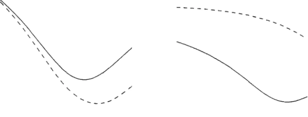
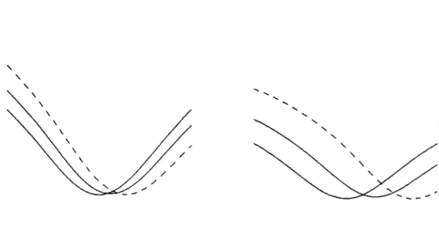
Figure 3 illustrates the maturity effect when Q(t, T) =1= 1. For comparison, the

figure illustrates also the smiles that obtain from preference-free option pricing à

la Hull-White. The latter smiles are distinguished by their symmetry. The solid lines are the implied volatility curves for a one-period option whereas the dashed lines are for a two-period option. The left and right panels are associated with

states 1 and 2, respectively, as the current state. It is seen that the maturity effect

depends on the current state: when state 1 is operative at time t, an increase in

maturity results in fiatter yet greater implied volatilities, while when in state 2

the fiatter implied volatility curves associated with longer maturities are lower. It

should be noticed that the smiles are moving to the right in both states. If one

considers the expressions developed in section 5.2, this is indicative of a negative skewness or leverage effect due to the persistence that we assumed for both states.

Next consider the case where B(t, T) is stochastic and Q(t, T) =1= 1. The lines

and panels of Figure 4, similar to those of the preceding figure, illustrate this case. Comparing the respective lines of figures 3 and 4, reveals that stochastic interest rates imply greater asymmetry in the smile. This is consistent with the presence

of a non-zero covariance between B(t, T) and the stock as illustrated in equation

(4.10).

An important remark is that at longer maturities, the smile is more asym-metric than at shorter maturities. This feature is apparent by noticing the point of intersection between the symmetric and asymmetric smiles at the respective maturities.

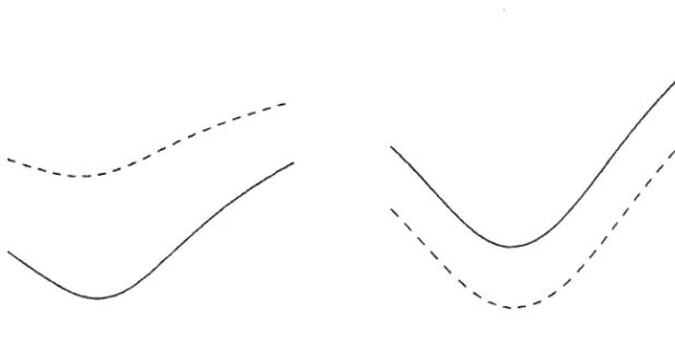
A verage duration and correlation effects Figures 5 and 6 illustrate the effect of changes in the persistence of each state on the implied volatility curves. Figure 4 considers the case where the probability of staying within a given state is

greater than its exit probability, Pii

>

Pij. The dashed lines represent an increase

in Pii from 0.8 to 0.9 and, as previously the left and right panels are associated

with states 1 and 2, respectively, as the current states. From each panel it is seen

that an increase in the persistence, or average duration (1 - Pii)-l, of each state

results in a greater asymmetry of the smile. It is interesting to note from the right

panel of Figure 4 that frowns obtain. In Figure 6 we consider the diametrically

opposite case where Pii

<

Pij. Increasing Pij from 0.8 to 0.9 in this case has the

same effects in terms of asymmetric distortions of the smile as in Figure 4 but with the roles of current state reversed: Frowns in this case arise when state 1 is

the time t operative state.

Figure 7 graphs the schedule of option prices across moneyness for two extreme

values of PXY the correlation between consumption and dividends. The solid line

represents the case PXY

=

1 while the dashed line is for PXy

=

o.

Regardless

of which state is operative at time t, an decrease in the correlation between

•

Leverage effects As we have seen, the preference-free option pricing formula à

la Hull-White obtains when there are no leverage effects, neither through the

mar-ket risk nor through the-stock risk., that is, when l(Xt, YtIU[) = l(Xt, YtlUi-1).

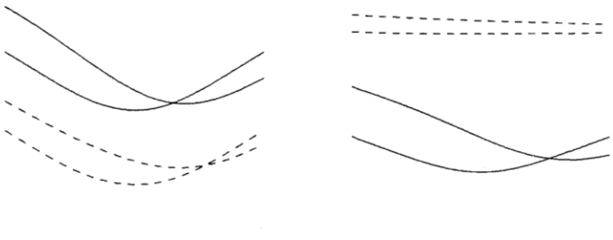
Figures 8 and 9 illustrate the implications that these leverage effects separately have in terms of the volatility smile. These implications are explored in the con-text of a two-period option which is the shortest horizon one can consider here since for a single-period option, absence of leverage through the stock risk im-plies Black-Scholes pricing. We preferred to keep the maturity horizon as short as possible in order to minimize the computation time.

In Figure 8 the dashed lines show the implications that an absence of leverage

through the consumption process has on the volatility smile., Le. l(XtIU[) =

l(XtIUi-1

). The solid lines are the benchmark case of leverage effects through

both the consumption and dividend processes. Notice that the symmetric smiles

resulting from preference-free option pricing à la Hull-White are identical whether

or not there is leverage through consumption. Absence of leverage through the consumption process leads to a more asymmetric smile as is apparent from both panels of the figure that, as before, are conditional on the current operative state. Similarly, in Figure 9 the dashed lines show the effect of an absence of

lever-age through the dividend process., Le. l(ltIU[)

=

l(ltlUi-1_{). Again we observe}

an asymmetric smile, except that in this case the asymmetric distortion is far more pronounced than in the previous figure. In other words, leverage through the divided process plays a much more important role than that through the consumption process insofar that the symmetry of the smile is concerned.

6.2.3. Preferences and smile effects

We now proceed to investigate the role played by the preference parameters. We will see that preferences, in particular intertemporal substitution, can have an effect in terms of the asymmetry of the volatility smile but that they play a secondary role compared to that played by the state variable. This is reassuring if one believes that such parameters should stay relatively stable over time. The benchmark for comparison here is the expected utility case which obtains when

, =

1. This was in fact the case up to this point. For example, recal! that the