A Work Project, presented as part of the requirements for the Award of a Masters Degree in Finance from the NOVA – School of Business and Economics

(1)

IS THE BASEL III LEVERAGE RATIO COUNTERCYCLICAL? A STUDY FOR PORTUGUESE BANKS1

Dina Raquel Pereira Batista - Student Number 835

A Project carried out on the Masters in Finance course, under the supervision of: Professor Doutor Paulo Pinho

June 2015

1

I would like to thank Banco de Portugal for all its support (also financial), in particular my hierarchy, and to Professor Doutor Paulo Pinho, Professor Doutor Manuel Vilares and Professor Doutor Maximiano Pinheiro for their trust and friendship.

I dedicate this work, and my best, to my kids, Diogo and Sara.

To Pedro, who held me through during this process, a hug, a kiss and a dance? To my parents, Maria Luisa e José Eugénio, my sister Salomé and lovely Mia, my brother João Pedro and my friend Isabel, my special thanks for all the times they supported me.

Finally, I should say that, if it takes a village to raise a child (African proverb), it also took a lot of good

friends to help me finish this business – João, Rodrigo, Simone, Luís, Barata, Fátima, Ana, Vítor,

(2)

Is

the Basel III leverage ratio countercyclical? A study for Portuguese

banks

Abstract

This work analyses how the leverage ratio behaves through the cycle, vis-à-vis other capital ratios. For a sample of the largest Portuguese banks, the Basel III leverage ratio is indeed countercyclical. This result is relevant from a regulatory perspective, since the introduction of a limit on the leverage ratio will function as a restriction in the banks’ balance sheet size, reducing the economic costs associated with the excessive growth of leverage in periods of economic expansion followed by aggressive deleveraging in the downturn. However, one cannot exclude that restrictions on banks’ leverage incentivize its transference to less regulated intermediaries.

JEL classification: E52, C32, E44, G28

(3)

1. Introduction

The basic concept underlying financial theory is that risk and expected return move together, which is to say, in an efficient market you can only expect more return if you take more risk.

Leverage, however, can mask the relationship between risk and return, in particular for banks, which typically hold only a relatively small portion of capital relative to assets. In fact, the banking sector has benefited from implicit public guarantees, not only regarding deposits but also against failure altogether, in particular banks that are regarded as “too big to fail”2. As a consequence of these implicit guarantees, banks have benefited from the upside of risk (return) while tax payers have borne the down side, leading to a classic moral hazard situation and an incentive for excessive risk taking (Adrian and Shin, 2008).

As a matter of fact, banks have historically operated with low levels of capital vis-à-vis assets (Admati et. al., 2013), despite being one of the most regulated industries. Furthermore, research conducted in ten European countries shows that capital to asset ratios have been on a long-term decline (Benink and Benston, 2005). Starting with around 30% capital in 1850-1880, the average ratio declined to about 15% in 1915-1933, 7.5% in 1945, 5-6% through 2001, and around 3% just before the financial crisis. This structural decline in capital levels has been attributed to factors such as looser

22

(4)

regulation, the increase in implicit guarantees from the government, higher cost of capital, the role played by large banks and increases in diversification3.

The financial crisis which started in 2007 and its enormous economic consequences have fuelled the discussion about the reliability of the pre-crisis regulatory framework, largely based on risk weighted capital requirements. Moreover, it should be noted that risk weights are dependent of general economic conditions and, as a consequence, are subject to cyclical fluctuations (Daníelsson 2001).

In this vein, among a large set of reforms, the Basel Committee of Banking Supervision (BCBS) is considering the introduction of a simple, risk-insensitive capital requirement, the leverage ratio (LR), which is regarded as a backstop measure to the risk weighted capital requirements and a guard against the build-up of excessive leverage, a key cause of the global financial crisis (BCBS, 2014).

Nevertheless, the leverage ratio also has its own drawbacks; most importantly, the leverage ratio is insensitive to assessments of the riskiness of different assets and used on its own can incentivize banks to arbitrage regulation by taking on riskier assets. It can also have unintended consequences in inducing a shift of activities with low measured risk to less regulated sectors (Acharya et al., 2012). Some research also suggests that bank portfolios could become more similar to one another and therefore more correlated, which could undermine financial stability, unless model risk is low or leverage requirements sufficiently high (Kiema and Jokivuolle, 2014).

3

(5)

The present definition of the leverage ratio includes total assets; derivatives; securities financing transactions and off balance sheet items in the denominator and Tier14 capital as numerator.

The main purpose of this work is to assess whether, in the case of the Portuguese banking sector, the Basel III LR is a countercyclical capital requirement. It also assesses whether it is more countercyclical than the accounting leverage (Tier/Assets) and the risk weighted ratio (Tier1/Risk weighted assets), in the sense that it is a tighter constraint in booms and a looser constraint in recessions.

It should be noted that, for the purpose of this work, pro-cyclicality refers to the mutually reinforcing mechanisms between the financial and real sectors of the economy which tend to amplify business cycle fluctuations and cause or exacerbate financial instability (Financial Stability Forum, 2009). Hence, if the leverage ratio is a countercyclical capital requirement, the ratio is expected to decrease as the cycle variable increases and vice-versa.

The model detailed in section 4 compares the behaviour of different capital ratios along the business cycle. These ratios have the same numerator (Tier 1) and different denominators (risk weighted assets, total assets and the BCBS leverage exposure measure) and several cycle measures were also tested (nominal GDP, real GDP and the credit-to-GDP gap) in order to have a comparable conclusion.

Nonetheless, the extensive literature summarized in section 3 mainly focus on the relationship between banks assets and their leverage. Moreover, the leverage is usually measured as the ratio of assets over capital, excluding some components of the BCBS LR.

4

(6)

The remainder of the work is structured as follows: section 2 presents a brief overview of the regulatory framework; section 3 comprises the literature review; the model, the empirical specification and the results obtained for the larger Portuguese banks are presented in section 4. Section 5 concludes.

2. Regulatory framework

The objective of the regulatory capital framework is to ensure that there is sufficient capital for banks to absorb unexpected losses and continue lending in a stress (BCBS, 2010).

This framework has evolved from a simplified Basel I approach, with few risk buckets, to a Basel II, 2.5 and III, increasingly more complex and risk sensitive

(Haldane and Madouros, 2012), largely based on banks’ internal models5

. Regardless of this increasing sophistication, banks have continued to fail and in the recent financial crisis, the amount of public support has been paramount, as well as the costs for the non-financial sectors, which have not yet fully recovered. According to Reinhart and Rogoff (2009), banking crises are associated with profound declines in output and employment6.

In the aftermath of the financial crisis that started in 2007, the regulatory reform has targeted the insufficiencies in regulation and supervision that were brought to light, since banks whose (risk weighted) capital ratios were well above minimum requirements collapsed, leading to public support or outright failure.

5

It should be noted that there was no effective international standard, since the degree of implementation of Basel II varied across jurisdictions and national supervisory authorities had a reasonable degree of discretion.

6

(7)

Furthermore, this financial crisis also highlighted that assessing the solvability of individual institutions is not a sufficient condition to financial system stability, albeit it is an essential one. In fact, problems arising in one institution can easily spread to other institutions or to the whole system via interconnectedness or common exposures, alongside with liquidity drying in financial markets, which is the modern equivalent of a bank run (BCBS, 2010). The possibility of such occurrence is usually referred to as “systemic risk”7.

The “lessons from the crisis” include, among other very relevant conclusions, the statement that there is a strong relation between risk-weighted capital requirements and the business cycle. Since internal models reflect past realizations of default rates (PD) and losses (LGD), in “good times the estimated losses and, consequently, capital requirements tend to be low”, in particular after a period of reduced volatility (Adrian and Shin, 2010). Additionally, since severe financial crisis are relatively rare and the models incorporate only a limited number of observations past crises tend not to be reflected in estimates of future losses (short term bias)8

. Moreover, there is a lag between the occurrence of facts that influence PD and LGD and the correspondent incorporation in those estimates.

The introduction of a simple, risk-insensitive capital requirement, the LR, which is not subject to the same cyclical fluctuations of risk weighted capital requirements, is regarded as a backstop measure to the latest and a guard against the build-up of excessive leverage, a key cause of the global financial crisis (BCBS, 2010).

7

Article 2- c) of Regulation (EU) 1092/2010 defines systemic risk as “a risk of disruption in the financial

system with the potential to have serious negative consequences for the internal market and the real economy”.

8

(8)

In particular, as risk weighting relies on knowable and quantifiable risks, there is a possibility that the assumptions underlying banks’ risk models or the standardized approach are not satisfied in the real world. Uncertainty and the possibility of structural breaks mean that the distributions of PD and LGD might not be fully known for certain types of exposures. Dermine (2014) shows that the LR limits the risk of a bank run when there is imperfect information on the value of a bank’s assets. Similarly, models are simplifications of the real world and the ways in which they are simplified may lead to mis-calibration (Daníelsson 2001). In this sense, the LR can help to protect against ‘unknown unknowns’, the proverbial black swan in the tail of the probability distribution.

In January 2014, the BCBS published the present definition of the leverage ratio. According to this definition, the capital measure is Tier 1 and the exposure measure comprises (i) on-balance sheet assets (excluding financial derivatives and securities financing transactions (SFT)9); (ii) off-balance sheet items (OBS) weighted according to the respective probability of being converted into on-balance sheet assets; (iii) financial derivatives, including the potential future exposure and (iv) SFT, comprising the counterparty credit risk. Netting between assets and liabilities is not permitted and risk mitigants (like collateral) are disregarded.

Although this definition of the LR is not yet final10

and the eventual requirement of a minimum LR will only be decided in 2017, with a view to an eventual migration to

9

SFT, usually referred to as repo-like transactions, include repos, reverse repos and securities lending. 10

(9)

Pillar I requirement in 2018, the impact assessment exercise has started in 2010, with a minimum reference level of 3%.

3. Literature Review

Most empirical studies conclude that bank leverage is pro-cyclical regarding banks’ assets, in particular for determined business models [investment banks (Adrian and Shin, 2008 and Baglioni et al., 2011) or banks especially involved in securitizations (Becalli et. al., 2014)] or large banks (Kalemli-Ozcan et. al., 2012).

The papers by Adrian and Shin (2008, 2010, 2013) study the cyclical behaviour of American banks balance sheet leverage. Their work is considered seminal and has been commonly used as a benchmark. Adrian and Shin (2008) shows that leverage (defined as assets/capital) is countercyclical for households, a-cyclical for commercial banks and pro-cyclical for investment banks.

For these investment banks, who keep mainly marked to market balance sheets, the authors conclude that the main determinant of leverage is their borrowing conditions, namely the haircuts on repo transactions. Additionally, the authors find a link between financial intermediaries’ balance sheet management and the markets’ perception of aggregate risk, measured by volatility11. When market asset prices rise and aggregate perception of risk is low, financing conditions are favourable and banks expand their balance sheets, mostly with recourse to very short term debt. The rate of growth of the aggregate financial sector balance sheets can be understood as the supply of aggregate liquidity; hence, the individual balance sheet management of financial intermediaries translates into credit growth (as more borrowers get credit when the banks’ balance sheet expands) and credit crunches (when financial intermediaries need do reduce their

11

(10)

balance sheet size). As a consequence, there are negative externalities from this profit seeking individual behaviour.

In Adrian and Shin (2013), the link between the value-at-risk (VaR) per unit of capital disclosed by banks and their leverage fluctuations is explored. Since VAR is determined for a given probability of failure (usually 1%), a capital stock and the underlying characteristics of assets (volatility, correlations), leverage behaviour can be mimicked assuming that financial intermediaries try to maintain this probability constant, perhaps in order to keep external ratings and creditworthiness. Hence, when volatility is low, the VaR per unit of assets (“unit VAR”) decreases and banks have “space” to grow their balance sheets. They do so by increasing their short term financing (repos, hedge funds cash management) and applications (reverse repos). It should also be noticed that the “unit VAR” can be interpreted as the required capital for banks per unit of asset, which corresponds to the medium risk weight in solvency regulation.

(11)

banks’ shareholders get only the upside of increasing risk taking and thus have an incentive for this behaviour12.

Baglioni et al. (2011) build on Adrian and Shin (2008) analysis, while investigating a sample of 77 major European banks (the Stoxx600 banks index) from 2000 to 2009. In Europe, the predominant type of bank is “universal”; hence the authors have distinguished “investment banks” and “commercial banks” by using the median ratio between interest income and net revenues (56%). Banks were classified as “commercial banks” if their ratio was above median. The authors conclude that (mainly) “investment banks” respond to a change in their assets value by changing leverage in the same direction, that is, leverage is pro-cyclical, which confirms Adrian and Shin (2008) results.

Becalli et. al. (2014) focus on the influence of off balance sheet items (in particular securitization) on leverage, building a measure of “effective leverage” that includes off-balance sheet securitizations, which compares with “formal” leverage (on off-balance sheet assets). Among other findings, the authors conclude that formal leverage underestimates effective leverage, and that not only investment banks but also commercial banks which are more involved in securitization have procyclical leverage. It should be noted that this is an approach to the present BCBS of the leverage exposure measure, since off balance sheet commitments are included in this exposure.

Galo and Thomas (2013) use a general equilibrium model to explore the relationship between bank leverage, GDP and capital and conclude that the volatility and pro-cyclicality of leverage can be understood as the result of the interplay between collateralized bank debt, moral hazard and changes in uncertainty. Since a significant

12

(12)

share of banks’ liabilities has limited liability, banks enjoy the upside risk in their assets, leaving the institutional investors to bear downsize, which is a classic moral hazard problem that induces banks to increase their debt and invest in riskier assets. In order to induce each bank to invest efficiently, investors monitor banks’ leverage ratios. If the uncertainty regarding banks’ assets returns increases, banks have an incentive to invest in riskier projects and investors will require a lower target leverage in order to prevent them from doing so. This deleveraging forces banks to contract their balance sheets leading to a fall in intermediated credit.

Fostel and Geanakoplos (2013) summarize several researches on the leverage cycle developed using a general equilibrium model is based in the relationship between leverage and collateral, since leverage can be obtained as the inverse of the haircut on collateral (for repo-like transactions). Volatility is a proxy for the fear of default and haircuts applied to the collateral are dependant of this perception of risk. Hence, fluctuations in volatility (like in the VIX index) can trigger adjustments in leverage. As in Adrian and Shin (2008), the conditions of credit to financial intermediaries determine their leverage. Authors conclude that the demand for collateral can origin bubbles in asset prices, which reinforce the leverage cycle, which is up when volatility is low, hence, in determined conditions, leverage can be determined endogenously.

(13)

measure definition which determine a different sensitivity to the cycle, it concludes that off-balance sheet items (OFS), like guarantees and other elements (credit lines, acceptances and items related to securitizations), are the items that give origin to the more procyclical behaviour of the Basel III exposure measure, which is in line with Becalli et. al. (2014) and their findings regarding the inclusion of securitizations in the “effective leverage”. The authors also conclude that results are different in “normal times” as compared with the crisis period, specifically; all capital ratios tend to be less countercyclical (more procyclical) during the crisis period. This might be explained by the reduced correlation of the denominator (which includes lending) with the cycle measures associated with the recognition of crisis-related losses or banks’ need to deleverage resulting from debt-overhang.

The cyclicality of capital, on the other hand, has been less studied and appears to be a-cyclical, at least during expansions, which means that banks do not accumulate capital in “good times” (Brei and Gambacorta, 2014).

The empirical specification used in this work adapts the model used in Brei and Gambacorta (2014) to the Portuguese banking sector and assesses whether the authors’ results hold.

4. Empirical Specification

(14)

were considered, namely, (a) the annual growth rate of nominal GDP (expressed in national currency); (b) The annual growth rate of real GDP; and (c) The credit-to-GDP gap (the difference between the credit-to-GDP ratio and its trend). The empirical specification follows Ayuso et al. (2004) and can be derived from a model in which a representative bank minimizes its intertemporal costs of capital.

The dynamic panel regression, broken down by bank, is designed to test how the different capital ratios correlate to the cycle:

= + + + ∗ + + ∗ + + ∗ +

The dependent variable, L is the capital ratio in year t, of bank i. As mentioned above three capital ratios are tested: the Basel III Leverage; the accounting leverage ratio and the capital-to-risk-weighted-assets ratio (Tier 1/Risk-weighted assets); α is a bank-specific constant which measures time invariant fixed effects; C is a dummy variable that accounts for the crisis period, as well as for the beginning of the adjustment towards the new regulatory standards – in Portugal, the dummy has been attributed a value of 1 from the last quarter of 2008 until the first quarter of 2014, since the crisis was prolonged by the sovereign debt crisis. The inclusion of L acknowledges the persistence in capital ratios, that is to say, the existence of short term adjustment costs. Y is the cycle explanatory variable.

As stated above, three cycle variables are being considered, namely, the annual growth rate of nominal GDP (expressed in national currency); the annual growth rate of real GDP; and the credit-to-GDP gap. The first two are business cycle measures, while the last one is a financial cycle proxy.

(15)

by the log of total assets; bank’s provisions over loans (P ) measure the relative riskiness of the bank and the return on assets ( ROA ) measures the direct cost of remunerating capital.

Hence, if the leverage ratio is a countercyclical capital requirement the results will yield a negative value for " . As a consequence, when the nominal GDP has positive growth rates, the leverage ratio will decrease and may become binding, thus requiring the bank to decrease its leverage exposure or increase its capital.

Additionally, if it is the more countercyclical of the capital ratios being tested, χ$ %& /(%)%&*+% ,-./01&% < χ$ %& /$/ *3 400% 0< χ$ %& /564, which means that the

leverage ratio is more sensible to the cycle, thus being the first capital requirements to signal the need for corrective action from the bank. In this sense, it would be the a tighter constraint in booms and a looser constraint in recessions

Finally, the effect of the crisis and innovation in banks’ regulation is also tested (by testing the statistical significance of "∗0).

One possible identification problem is endogeneity, originated either from misspecification of the model (omitted variables) or from simultaneity among variables, since the state of the banking sector could also affect the business cycle and the credit cycle.

(16)

In order address the second question, different lags of the endogenous variables are also used, since instrumental bank-specific characteristics are lagged by one year in order to mitigate the possible endogeneity problem.

4.1.Data

For the estimation of the empirical model, quarterly supervisory bank level data for Tier 1 capital, total assets, risk weighted assets, financial derivatives, securities financing transactions; off balance sheet items (guarantees and commitments), profits, total credit and provisions were used. When quarterly data is not available, linear interpolation of annual or semi-annual data was used. Observations cover the period from 2000Q4 to 2014Q1. The cut-off dates correspond to the availability of consistent data in the beginning of the period and the choice of 2014Q1 precludes including the data break associated with the resolution measured applied to Banco Espiríto Santo, SA in August 2014. The exact availability of data is disclosed in Annex II, as well as the methodology used to estimate the exposure measure of the LR.

Quarterly nominal and real GDP data are from the National Statistics Institute (INE) and the series used refer to ESA 1995 methodology. The credit-to-GDP gap was obtained from internal estimates of the Banco de Portugal13.

The sample includes the largest banking groups operating in Portugal, either regarding total assets or credit provisioning to the economy, namely, Caixa Geral de Depósitos (CGD); Banco BPI (BPI); Banco Comercial Português (BCP); Banco

13

(17)

Espírito Santo (ES); Banco Santander Totta (BST) e Caixa Económica Montepio Geral (CEMG). Despite its relevance to the Portuguese banking sector, Banco Internacional do Funchal (BANIF) was excluded from the sample, due to extreme variations in capital ratios that could not be attributable to cyclical effects.

Table 1 presents a summary characterization of the main variables, namely, capital ratios and business cycle measures. It can be observed that nominal and real GDP growth rates during the crisis period were negative (-0.002;-0.003), while all the capital ratios present a higher average during this period. It should also be noted that the credit gap depicts a negative mean during the crisis, revealing the tightening of credit supply to the economy.

Table 1 – Data summary

Variable Mean Std.

dev Min Max Variable Mean

Std.

dev Min Max

Capital Ratios Cycle Variables

Tier 1/Leverage

exposure 0.053 0.011 0.030 0.082

Nominal GDP

growth 0.005 0.010 -0.022 0.026

Tier 1/Leverage exposure - Crisis

0,059 0,010 0,039 0,082 Nominal GDP

growth – crisis - 0,002 0,011 - 0,022 0,014

Tier1/ Total

Assets 0.056 0.011 0.034 0.086

Real GDP

growth -0.000 0.008 -0.024 0.147

Tier1/ Total

Assets – Crisis 0,064 0,010 0,044 0,086

Real GDP

growth – crisis - 0,003 0,009 - 0,024 0,011 Tier 1/Risk

weighted assets 0.086 0.021 0.050 0.162

Credit Gap (in

differences) 0,001 1,763 - 3,583 4,299

Tier 1/Risk weighted assets - Crisis

0,102 0,020 0,065 0,162

Credit Gap (in differences) - crisis

- 0.248 1,748 - 3,583 3,747

4.2.The cyclicality of capital ratios

(18)

the other cycle measures outcomes are presented in annex I. Additionally, the t-test on the difference in the mean between Tier/Exposure measure and Tier1/Total assets indicates that the two capital measures are statistically different (the results for the t-test are also presented in annex 1).

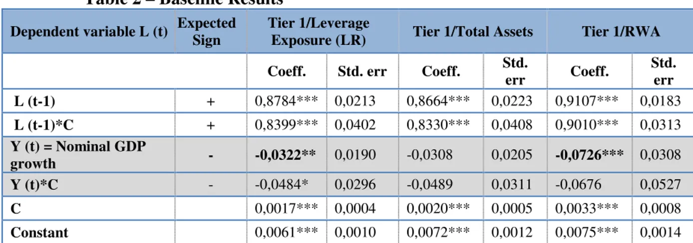
Table 2 – Baseline Results

Dependent variable L (t) Expected

Sign

Tier 1/Leverage

Exposure (LR) Tier 1/Total Assets Tier 1/RWA

Coeff. Std. err Coeff. Std.

err Coeff.

Std. err

L (t-1) + 0,8784*** 0,0213 0,8664*** 0,0223 0,9107*** 0,0183

L (t-1)*C + 0,8399*** 0,0402 0,8330*** 0,0408 0,9010*** 0,0313

Y (t) = Nominal GDP

growth - -0,0322** 0,0190 -0,0308 0,0205 -0,0726*** 0,0308

Y (t)*C - -0,0484* 0,0296 -0,0489 0,0311 -0,0676 0,0527

C 0,0017*** 0,0004 0,0020*** 0,0005 0,0033*** 0,0008

Constant 0,0061*** 0,0010 0,0072*** 0,0012 0,0075*** 0,0014

All estimations are based on the Arellano and Bover (1995) system GMM estimator. ***, **, * indicate significance at the 1%, 5%, and 10% level. Bank fixed effects are not reported.

By the observation of the table above, one can conclude that:

(i) The LR varies in opposite relation with nominal GDP (χ$ %& /,-.< 0 , while

this is not the case when considering the ratio Tier 1/Total Assets.

(ii) During the crisis period, only the leverage ratio coefficient is statistically different from zero and negative, indicating that the ratio is countercyclical (χ ∗$ %& /,-.< 0 .

(19)

This result can be explained by the fact that risk-weighted capital requirements are subject of regulatory constraints, which increased during the crisis (hence, TIER 1/RWA increased while nominal GDP presented negative growth rates) leading to a countercyclical behaviour. This is a classical case for the Lucas critique, since we are observing a variable which is subject to policy restrictions. By contrast, the LR was not subject to restrictions or close monitoring.

Additionally, Portuguese banks have changed their balance sheet composition, moving away from assets with non-zero risk weights towards sovereign debt (with an associated zero risk weight). Hence, leverage exposure growth has been more pronounced than risk weighted assets increase, as can be observed in graph 1. Once again, this was possible because leverage is not regulated and, furthermore, no bank in the sample would fail the 3% threshold which has been tested in Basel II quantitative impact assessment (as is depicted in table 1).

Graph 1 – Leverage exposure measure and risk weighted assets

(iv) All the capital ratios are time persistent. As a matter of fact, 0.87 of the LR in a given period can be explained by its value in the previous quarter. The coefficient for the risk weighted capital ratio in even higher (0.91).

(20)

(v) It should also be noticed that the coefficients for the crisis dummy are always statistically different from zero and positive. This can be explained by increased capital requirements during the post-2008 period, which translate in a 0.002 coefficient for the LR and a 0.004 coefficient for the RWA ratio.

(vi) Coefficients for the real GDP growth as cycle measure are not statistically different from zero for all the capital ratios and the coefficients for the credit gap are all very close to zero. These results are presented in annex I.

As can be observed in table 3, the inclusion of bank specific characteristics does not change the main conclusions presented above. This can be interpreted as a similitude between the business models of the several banks in the sample, which indeed are all universal banks, despite differences in the total share of the market and even in risk taking and balance sheet composition.

It should also be highlighted that the size coefficient is not statistically different from zero for the complete sample, hence one can assume that the “too big too fail” subsidy is independent of the bank size or that it is not relevant. On the other hand, in the crisis period this coefficient becomes statistically significant for all the business cycle measures, perhaps due to greater scrutiny and requirements by the supervisor concerning larger banks, which were also recapitalized, either with public (BCP, CGD and BPI) or private capital (ES). Additionally, it can be argued out that the implicit public subsidies are bigger during crises, when the likelihood of failure increases.

(21)

Table 3 – Controlling for bank specific characteristics Dependent variable L (t) Expected

Sign Tier 1/Leverage _Exposure Tier 1/Total Assets Tier 1/RWA

Coeff. Std. err Coeff. Std. Err Coeff. Std.

err

L (t-1) + 0,8652*** 0,0237 0,8479*** 0,0248 0,8926*** 0,0208

L (t-1)*C + 0,7757*** 0,0512 0,7394*** 0,0551 0,8641*** 0,0411

Y (t) = Nominal GDP

growth - -0,0327* 0,0190 -0,0288 0,0205 -0,0718** 0,0309

Y (t)*C - -0,0427 0,0294 -0,0362 0,0309 -0,0577 0,0533

C 0,0015** 0,0005 0,0016*** 0,0006 0,0036*** 0,0009

Size (t-1) 0,0008 0,0005 0,0013 0,0006 -0,0007 0,0009

Size (t-1)*C 0,4668*** 0,1915 0,1167*** 0,0360 0,1036* 0,0605

ROA(t-1) 0,2673** 0,1208 0,2996 0,1303 -0,0074 0,1904

ROA(t-1)*C 0,0831*** 0,0323 0,0012 0,0012 0,0017 0,0021

%Prov. (t-1) 0,0340** 0,0161 0,0439*** 0,0177 0,0384 0,0269

%Prov. (t-1)*C 0,0049 0,0131 -0,0004 0,0137 -0,0069 0,0238

Constant -0,0027 0,0059 -0,0070 0,0062 0,0150 0,0099

All estimations are based on the Arellano and Bover (1995) system GMM estimator. ***, **, *indicate significance at the 1%, 5%, and 10% level. Bank fixed effects are not reported.

4.3.The cyclicality of the components of the capital ratios

A capital ratio can change by altering either the numerator or the denominator, hence it is relevant to analyse separately the cyclical behaviour of the numerator (Tier 1) and the denominators (leverage exposure, total assets and risk weighted assets). The specification of the model is the same as the one in section 4.1, with minor adaptations. Since the logarithmic transformation did not yield stationary variables, differences were used in order to avoid spurious regressions, corresponding to these variables growth rates.

(22)

reform addresses this undesirable effect by imposing a countercyclical capital buffer, which is constituted in the upswing and can be depleted during downturns14.

Results for the leverage exposure and total assets are statistically significant for the crisis period, during which they show a countercyclical pattern, while when considering the complete sample period, the sign of the corresponding coefficients signal procyclical behaviour. Risk weighted assets are significantly procyclical when considering the entire sample period, but countercyclical during the crisis.

Table 4 – Cyclicality of the components of the capital ratios Dependent

variable L (t) Tier 1 (growth) Leverage Exposure _(growth) Total Assets _(growth) _{Assets (growth)}Risk Weighted

Coeff. Std. err Coeff. Std. err Coeff. Std.

err Coeff. Std. err

L (t-1) _0,9831*** _0,0087 _0,9895*** _0,0055 _{0,9933*** 0,0058 1,0071***} _0,0038

L (t-1)*C _0,9834*** _0,0178 _0,0552*** _0,0048 _{0,0480*** 0,0040 0,0670***} _0,0059

Y (t) = Nominal GDP growth

-0,9433*** 0,3197 0,1439 0,1731 0,1628 0,1799 0,3832*** 0,1234

Y (t)*C _-1,0157** _0,5187 _{-1,6865*** 0,4602} _-0,7553** _{0,3718 -0,3004} _0,5142

C _-0,0068 _0,0086 _0,1852 _0,0511 _-0,0084** _{0,0042 -0,0245*** 0,0027}

Constant _0,1524** _0,0641 _0,0000 _0,0000 _0,0849 _{0,0605 -0,0555} _0,0383

Using the credit gap as the cycle variable yields differentiated results, since all components are pro-cyclical and the coefficients are statistically significant.

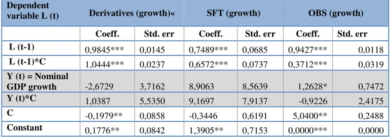
4.4.The cyclicality of the leverage exposure components

Since the leverage ratio exposure measure builds on total balance sheet assets, while including additional components that increase the risk of eventual excessive leverage, namely, the potential future exposure of derivative contracts, the counterparty credit risk of securities financing transactions (SFT) and the conversion of off-balance sheet items

(23)

(OBS), guarantees and commitments, into on balance sheet components it is relevant to consider each one specific contribution to the cyclicality of the exposure measure (and the leverage ratio). The results of an econometric specification analogous to the one presented in section 4.3 are presented in table 5.

It can be observed that the only component that exhibits a procyclical pattern is OBS, which is positive and statistically different from zero. This component also shows a countercyclical behaviour during the crisis, perhaps due to the conversion of banks’ commitments and guarantees or to more risk aversion from the banks when entering into these operations.

The derivatives and SFT components do not present statistically significant coefficients.

Table 5 – Cyclicality of the components of the leverage exposure Dependent

variable L (t) Derivatives (growth)« SFT (growth) OBS (growth)

_Coeff. _{Std. err} _Coeff. _{Std. err} _Coeff. _{Std. err}

L (t-1) _0,9845*** _0,0145 _0,7489*** _0,0685 _0,9427*** _0,0118

L (t-1)*C _1,0444*** _0,0237 _0,6572*** _0,0737 _0,3712*** _0,0319

Y (t) = Nominal

GDP growth -2,6729 3,7162 8,9063 8,5639 1,2628* 0,7472

Y (t)*C _1,0387 _5,5350 _9,1697 _7,9137 _-0,9226 _2,4175

C _-0,1979** _0,0858 _-0,3446 _0,6191 _5,0400** _0,2488

Constant _0,1776** _0,0842 _1,3905** _0,7153 _0,0000*** _0,0000

Since this work follows the study conducted in Brei and Gambacorta (2014), results can be compared with this benchmark. Several aspects can be pointed out:

(i) In both studies, capital ratios present a high degree of time persistency, which can be explained by adjustment costs, in particular when issuing additional capital. (ii) In both studies, the Basel II leverage ratio is countercyclical, as well as the

(24)

Portuguese case the LR is not more countercyclical than the risk weighted assets ratio. This result may be explained by the particular adjustment process that the Portuguese banking system undertook in recent years, as well as by historically low risk weighted capital ratios and relatively high average risk weights.

(iii)In both studies, the leverage exposure and total assets are counter-cyclical during the crisis period. On the other hand, Tier 1 is pro-cyclical in Grei and Gambacort (2014), while countercyclical for the Portuguese banking sector. This result can be explained by the capitalisation effort that has been undertaken in recent years, during which product growth was sluggish (in Portugal).

(iv) In both studies, off balance sheet items are the most pro-cyclical component of the Basel III leverage ratio exposure.

5. Conclusions

In an increasingly complex model of regulation, the leverage ratio is on the way of being introduced as a backstop measure to risk weighted capital ratios. At the present, some jurisdictions like Canada, United States Switzerland and the UK have already introduced a leverage restriction or recommendation via national legislation.

At international level, the BCBS is currently assessing the impact of introducing a 3% minimum requirement, while at EU level the European Commission is expected to deliver a report on the calibration of a possible binding Pillar I requirement by 2018. Hence, the subject merits being studied, as it will condition the future behaviour of bank managers.

(25)

bank leverage appears to behave cyclically because banks' assets and liabilities management decisions are mainly driven risk-adjusted regulatory capital adequacy requirements. When banks try to maintain a constant volume of risk-weighted assets through the cycle, bank leverage will vary with the cycle. In this context, a regulatory leverage ratio requirement may limit cyclicality of bank leverage.

Brei and Gambacorta (2014), is the first empirical experiment that assesses the behaviour of the leverage ratio over the economic cycle. Portugal is not included in the authors’ sample; nevertheless, if the requirement is imposed by European regulation, Portuguese banks will also be subject to it.

This work, in line with Brei and Gambacorta (2014), concludes that the leverage ratio is countercyclical. On the other hand, the results of this study do not convey that it is a tighter constraint in booms and a looser constraint in recessions that the risk weighted capital ratio.

(26)

References

Acharya, V., Mehran, H., Shuermann, T. and Thakor, A. (2012): Robust capital regulation, CEPR Discussion papers 8792.

Admati, A. R., Demarzo, P. M., Hellwig, M. F., & Pfleiderer, P. (2011). Fallacies , Irrelevant Facts , and Myths in the Discussion of Capital Regulation: Why Bank Equity is Not Expensive. Preprints of the Max Planck Institute for Research on Collective Goods Bonn 2010/42.

Adrian, T., & Shin, H. S. (2010). Liquidity and leverage. Journal of Financial

Intermediation, 19(3), 418–437.

Adrian, T., & Shin, H. S.. (2010), The Changing Nature of Financial Intermediation and the Financial Crisis of 2007-09. Federal Reserve Bank of New York Staff Reports (March).

Adrian, T., & Shin, H. S. (2014). Procyclical leverage and value-at-risk. Review of

Financial Studies, 27(2), 373–403.

Aikman, D., Galesic, M., Gigerenzer, G., Kapadia, S., Katsikopoulos, K. V, Kothiyal, A., … Neumann, T. (2014). Taking uncertainty seriously: simplicity versus complexity in financial regulation. Bank of England Financial Stability Paper, (28).

Ayuso, J., Pérez, D., & Saurina, J. (2004). Are capital buffers pro-cyclical? Evidence from Spanish panel data. Journal of Financial Intermediation, 13(2), 249–264. Baglioni, a., Beccalli, E., Boitani, a., & Monticini, a. (2013). Is the leverage of

European banks procyclical? Empirical Economics, 45(3), 1251–1266.

Banca D'Italia, Financial sector pro-cyclicality (2009), Occasional papers, Questioni di

Economi e Finanza, number 44.

Beccalli, E., Boitani, A., & Di Giuliantonio, S. (2014). Leverage pro-cyclicality and securitization in US banking. Journal of Financial Intermediation.

Brei, M., & Gambacorta, L. (2014). The leverage ratio over the cycle, (471). BIS

Working Papers, No 471 (November).

Cecchetti, S. (2011). How to cope with the too-big-to-fail problem? 10th Annual Conference of the International Association of Deposit Insurers, "Beyond the Crisis: The Need for a Strengthened Financial Stability Framework", Warsaw,

Poland, 19 October 2011.

(27)

Committee, B. (2010). Basel Committee on Banking Supervision, Basel III: A global regulatory framework for more resilient banks and banking systems

Drehmann, M. (2013). Total credit as an early warning indicator for systemic banking crises, Basel Committee on Banking Supervision, BIS Quarterly Review, June 2013.

Financial Stability Forum (2009). Report of the Financial Stability Forum on Addressing Procyclicality in the Financial System.

Fostel, A., & Geanakoplos, J. D. (2013). Reviewing the Leverage Cycle. Annual Review

of Economics.

Galo, N.&Thomas, C. (2013). Bank Leverage Cycles, Banco de Espana, Working Paper No. 1222.

Haldane, A. G., & Madouros, V. (2012). The dog and the frisbee. Federal Reserve Bank

of Kansas City’s 36th Economic Policy Symposium, 1–36.

Harald Benink and George Benston, “The Future of Banking Regulation in Developed Countries: Lessons from and for Europe,” Financial Markets, Institutions and

Instruments 14, no. 5 (2005): 289–327.

Kalemli-Ozcan, S., Sorensen, B., & Yesiltas, S. (2012). Leverage across firms, banks, and countries. Journal of International Economics, 88(2), 284–298.

Kierma, I. and Jokivuole, E. (2014). Does a leverage ratio requirement increase bank stability?. Journal of Banking and Finance 02/2014, 39, pages 240-254.

Merton, R., Theory of Rational Option Pricing. The Bell Journal of Economics and

Management Science, Vol. 4, No. 1 (Spring, 1973), pp. 141-183.

Regulation (EU) 1092/2010 of the European Parliament and of the Council (24 November 2010), on European Union macro-prudential oversight of the financial system and establishing a European Systemic Risk Board.

Regulation (Eu) No 575/2013 of The European Parliament and of The Council of 26 June 2013 on prudential requirements for credit institutions and investment firms and amending Regulation (EU) No 648/2012.

Reinhart, C. M., & Rogoff, K. S. (2009). The Aftermath Of Financial Crises. National

(28)

A Work Project, presented as part of the requirements for the Award of a Masters Degree in Finance from the NOVA – School of Business and Economics

ANNEX I: Results for alternative measures of the cycle variable Table 1a) Baseline regression/Cycle variable = Real GDP growth

Dependent variable L (t)

Expected Sign

Tier 1/Leverage

Exposure Tier 1/Total Assets Tier 1/RWA

Coeff. Std. err Coeff. Std. err Coeff. Std. err

L (t-1) + 0,8744*** 0,0212 0,8627*** 0,0222 0,9062*** 0,0183

L (t-1)*C + 0,8308*** 0,0401 0,8238*** 0,0407 0,8963*** 0,0314

Y (t) = Real GDP growth

- -0,0085 0,0203 -0,0107 0,0220 -0,0335 0,0332

Y (t)*C - -0,0229 0,0357 -0,0239 0,0374 0.0188 0.7654

C 0,0020*** 0,0004 0,0023 0,0004 0,0040*** 0,0007

Constant 0,0060*** 0,0010 0,0071 0,0012 0,0072*** 0,0014

Table 1b) Baseline regression/Cycle variable = Credit Gap Dependent

variable L (t)

Tier 1/Leverage

L (t-1) + 0,8753*** 0,0212 0,8643*** 0,0222 0,9065*** 0,0183

L (t-1)*C + 0,8128*** 0,0460 0,7964*** 0,0483 0,8483*** 0,0412

Y (t) = Credit Gap

- 0,0000 0,0000 0,0000* 0,0000 0,0000 0,0000

Y (t)*C - -0,0001 0,0001 -0,0001 0,0001 -0,0003* 0,0002

C 0,0012** 0,0007 0,0014** 0,0007 0,0032*** 0,0011

Constant 0,0020 0,0027 0,0026 0,0029 0,0026 0,0043

(29)

Table 2a) Controlling for bank specific characteristics/Cycle variable = Real GDP growth Dependent

variable L (t)

Tier 1/Leverage Exposure Tier 1/Total Assets Tier 1/RWA

L (t-1) + 0,8609*** 0,0236 0,8441*** 0,0247 0,8878*** 0,0209

L (t-1)*C + 0,7250*** 0,0542 0,2343*** 0,0192 0,8549*** 0,0408

Y (t) = Real

GDP growth - -0,0109 0,0204 -0,0123 0,0220 -0,0292 0,0332

Y (t)*C - -0,0080 0,0368 0,0215 0,0225 0,0339 0,0631

C 0,0018*** 0,0005 0,0019*** 0,0005 0,0042*** 0,0009

Size (t-1) 0,0008 0,0005 0,0013** 0,0006 -0,0006 0,0009

Size (t-1)*C 0,5751*** 0,2009 0,0033*** 0,0001 0,3625 0,3401

ROA(t-1) 0,2596** 0,1213 0,2939** 0,1309 -0,0227 0,1922

ROA(t-1)*C 0,1231*** 0,0359 1,0537*** 0,1300 0,1153* 0,0607

%Prov. (t-1) 0,0349** 0,0162 0,0449*** 0,0177 0,0403 0,0272

%Prov. (t-1)*C 0,0012 0,0012 0,3438* 0,0211 0,0017*** 0,0021

Constant -0,0031 0,0059 -0,0076 0,0062 0,0131 0,0099

Table 2b) Controlling for bank specific characteristics/Cycle variable = = Credit Gap Dependent variable L (t)

Tier 1/Leverage

Coeff. Std. err Coeff. Std. err Coeff. Std. err

L (t-1) + 0,8495*** 0,0239 0,8349*** 0,0249 0,8782*** 0,0208

L (t-1)*C + 0,7640*** 0,0506 0,7279*** 0,0539 0,8399*** 0,0441

Y (t) = Credit Gap - 0,0000** 0,0000 0,0000* 0,0000 0,0001*** 0,0000

Y (t)*C - 0,0001*** 0,0001 0,0001 0,0001 -0,0002 0,0002

(30)

Dependent variable L (t)

Tier 1/Leverage

Coeff. Std. err Coeff. Std. err Coeff. Std. err

Size (t-1) 0,0003 0,0006 0,0009 0,0006 -0,0014 0,0010

Size (t-1)*C 0,4675*** 0,1922 0,5892*** 0,2012 0,3614 0,3390

ROA(t-1) 0,2412** 0,1199 0,2775** 0,1295 -0,0535 0,1901

ROA(t-1)*C 0,1204*** 0,0431 0,1618*** 0,0467 0,0743 0,0727

%Prov. (t-1) 0,0481** 0,0172 0,0583*** 0,0189 0,0640** 0,0284

%Prov. (t-1)*C 0,0006 0,0011 0,0012 0,0012 0,0014 0,0021

Constant -0,0041 0,0059 -0,0086 0,0062 0,0108 0,0099

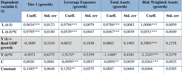
Table 3a) Cyclicality of the components of the capital ratios /Cycle variable = Real GDP growth

Dependent variable L (t)

Tier 1 (growth) Leverage Exposure

(growth)

Total Assets (growth)

Risk Weighted Assets (growth)

Coeff. Std. err Coeff. Std. err Coeff. Std. err Coeff. Std. err

L (t-1) 0,9634*** 0,0123 0,9794*** 0,0079 0,9788*** 0,0083 1,0006*** 0,0059

L (t-1)*C 0,9795*** 0,0180 0,0539*** 0,0047 0,0467*** 0,0039 0,0551*** 0,0049

Y (t) = Real GDP growth

-0,3889 0,3510 0,0632 0,1830 0,0803 0,1903 0,3903*** 0,1278

Y (t)*C -0,5071 0,6375 -1,9132* 0,5359 -1,1488* 0,4381 -2,3243*** 0,5379

C 0,0020 0,0081 -0,0099*** 0,0037 -0,0095** 0,0039 -0,0261*** 0,0025

Constant 0,1485** 0,0648 0,1292** 0,0575 0,0887 0,0604 -0,0466 0,0385

Table 3b) Cyclicality of the components of the capital ratios /Cycle variable = Credit Gap

Dependent variable L (t)

(growth) Total Assets (growth)

Risk Weighted Assets (growth)

Coeff. Std. err Coeff. Std. err Coeff. Std. err Coeff. Std. err

L (t-1) 0,9301*** 0,0142 0,9581*** 0,0099 0,9596*** 0,0104 0,9816*** 0,0077

L (t-1)*C 0,9863*** 0,0184 0,1234** 0,0156 0,1268*** 0,0150 0,1757*** 0,0158

Y (t) = Credit

(31)

Dependent variable L (t)

(growth) Total Assets (growth)

Risk Weighted Assets (growth)

Coeff. Std. err Coeff. Std. err Coeff. Std. err Coeff. Std. err

Y (t)*C 0,0022*** 0,0013 0,0639*** 0,0010 0,0639*** 0,0010 0,0637*** 0,0011

C -0,0238** 0,0106 -0,0262*** 0,0055 -0,0253*** 0,0057 -0,0430*** 0,0039

Constant 0,0752 0,0671 0,1701*** 0,0582 0,1309** 0,0612 -0,0159 0,0392

Table 4a) Cyclicality of the components of the leverage exposure/Cycle variable = Real GDP growth

Dependent variable L (t) Expected Sign Derivatives

(growth) SFT (growth)

Off-Balance Sheet Items (growth)

Coeff. Std.

err Coeff.

Std.

err Coeff. Std. err

L (t-1) + 0,9307*** 0,0237 0,5738*** 0,0808 0,9337*** 0,0152

L (t-1)*C + 1,0443*** 0,0237 0,6211*** 0,0720 0,3263*** 0,0270

Y (t) = Real GDP

growth + -0,5781 4,3938 -0,6044 10,1702 1,8183 0,8105

Y (t)*C + 2,9027 6,9578 5,4852 11,3075 -0,6236 2,5268

C -0,0147 0,1062 0,1414 0,5878 0,0197 0,0165

Constant 0,0876 0,2183 3,2089*** 0,9444 0,5011*** 0,1040

Table 4b) Cyclicality of the components of the leverage exposure/Cycle variable = Credit Gap Dependent variable L (t) Expected Sign Derivatives

(growth) SFT (growth)

Off-Balance Sheet Items (growth)

Coeff. Std.

err Coeff.

Std.

err Coeff. Std. err

L (t-1) + 0,9349*** 0,0237 0,5447*** 0,0799 0,9309*** 0,0153

L (t-1)*C + 1,0532*** 0,0281 0,4649*** 0,0895 0,3944*** 0,0341

Y (t) = Credit Gap + 0,0209*** 0,0081 0,0466* 0,0257 0,0007 0,0009

Y (t)*C + 0,0043 0,0028 0,0355*** 0,0054 0,0381*** 0,0018

C -0,4394** 0,1953 -0,3794 0,6440 -0,0086 0,0296

Constant

-2,8549*** 1,1509 -3,1288 3,6159 0,4001*** 0,1487

(32)

(33)

ANNEX II: Data sample and the estimate of the Leverage Ratio exposure measure

A. Data availability and source

Individual bank data from the supervisory reports to the Banco de Portugal was used in the empirical estimates; hence this data is confidential. In the most recent periods all the variables are available with quarterly frequency, nevertheless in the beginning of the period some of the variables are only available annually or semi-annually and quarterly data was obtained using linear interpolation. Table 5 depicts the availability of data on a bank basis.

It should also be stressed that the introduction of the IFRS did not cause a major time series break in what regards data used in this study, since the precious regime stipulated analogous rules regarding, inter alia, netting of exposures. Furthermore, Banco de Portugal has kept long time series of comparable data for the major banking groups, which are used in this work.

Nominal and real GDP are official statistics from the national statistics institute (INE), seasonally adjusted.

(34)

Table 5 Data availability per banking group

Source CGD BCP BPI BST CCAM CEMG ES SICAM

TIER 1

Supervisory reporting to Banco de

Portugal

2000Q4-2008Q4: Semi-annual data

2009Q1-2014Q1: Quarterly data

Risk Weighted Assets

Total Assets

Profits

Credit

Provisions

Financial

Derivatives 2008Q2-2014Q1: Quarterly data

Securities Financing Transactions

2007Q1-2014Q1 Quarterly

data

Guarantees

Cancellable Commitments

Uncancellable Commitments

Nominal GDP

INE 2000Q4-2014Q1: Quarterly data

Real GDP

Credit Gap

Banco de Portugal

internal estimates

B. Estimating the Leverage Ratio Exposure

(35)

(2014) and essentially estimates the relationship between the balance sheet exposure of derivatives and SFT with the add-ons for, respectively, potential future exposure (PFE) and counterparty credit risk and applies those coefficients to on-balance sheet exposure . Furthermore, in the case of derivatives, netting is not allowed, hence an additional coefficient for the relationship between balance sheet values and leverage exposure is also calculated.

The inclusion of off-balance sheet items (OBS) is one of the most striking features of the leverage ratio exposure, since recent history has proved that in moments of crisis off-balance exposure turns into on-balance. In the EU, OBS items will be included in the exposure of the leverage ratio via the use of the supervisory conversion factors in Annex I of the Capital Requirements Regulation (CRR), according to the likelihood that those items have of being converted into on-balance sheet items, ranging from 10% for cancellable commitments and 100% for full risk categories. The OBS considered are guarantees and commitments.

Table 6 Coefficients used to estimate the leverage exposure Exposure

item Coefficient Rationale

Expected

Value Estimate

Derivatives

A= 9:9; <= > ?@ABCDEBC@F GHIJFKA@

?@ABCDEBC@F DLLJKMEBMN ODPDML@ FQ@@E CDPK@ -1

Revert derivatives

netting

1≤ S ≤

015 -25%

B= 9:9; <= > ?@ABCDEBC@F TUG