Regulatory Networks
Yali Wang1*, Tong Zhou
1Department of Automation, Tsinghua University, Beijing, China, 2Tsinghua National Laboratory for Information Science and Technology (TNList), Tsinghua University, Beijing, China
Abstract
Gene regulatory network (GRN) reconstruction is essential in understanding the functioning and pathology of a biological system. Extensive models and algorithms have been developed to unravel a GRN. The DREAM project aims to clarify both advantages and disadvantages of these methods from an application viewpoint. An interesting yet surprising observation is that compared with complicated methods like those based on nonlinear differential equations, etc., methods based on a simple statistics, such as the so-calledZ-score, usually perform better. A fundamental problem with theZ-score, however, is that direct and indirect regulations can not be easily distinguished. To overcome this drawback, a relative expression level variation (RELV) based GRN inference algorithm is suggested in this paper, which consists of three major steps. Firstly, on the basis of wild type and single gene knockout/knockdown experimental data, the magnitude of RELV of a gene is estimated. Secondly, probability for the existence of a direct regulation from a perturbed gene to a measured gene is estimated, which is further utilized to estimate whether a gene can be regulated by other genes. Finally, the normalized RELVs are modified to make genes with an estimated zero in-degree have smaller RELVs in magnitude than the other genes, which is used afterwards in queuing possibilities of the existence of direct regulations among genes and therefore leads to an estimate on the GRN topology. This method can in principle avoid the so-called cascade errors under certain situations. Computational results with the Size 100 sub-challenges of DREAM3 and DREAM4 show that, compared with theZ-score based method, prediction performances can be substantially improved, especially the AUPR specification. Moreover, it can even outperform the best team of both DREAM3 and DREAM4. Furthermore, the high precision of the obtained most reliable predictions shows that the suggested algorithm may be very helpful in guiding biological experiment designs.
Citation: Wang Y, Zhou T (2012) A Relative Variation-Based Method to Unraveling Gene Regulatory Networks. PLoS ONE 7(2): e31194. doi:10.1371/ journal.pone.0031194
Editor:Frank Emmert-Streib, Queen’s University Belfast, United Kingdom
ReceivedOctober 5, 2011;AcceptedJanuary 4, 2012;PublishedFebruary 20, 2012
Copyright:ß2012 Wang, Zhou. This is an open-access article distributed under the terms of the Creative Commons Attribution License, which permits unrestricted use, distribution, and reproduction in any medium, provided the original author and source are credited.
Funding:The reported work was financially supported in part by the 973 Program under Grant 2012CB316504 and 2009CB320602 and by the National Natural Science Foundation of China under Grants 61174122, 61021063, 60721003 and 60625305. The funders had no role in study design, data collection and analysis, decision to publish, or preparation of the manuscript.
Competing Interests:The authors have declared that no competing interests exist. * E-mail: [email protected]
Introduction
In the post-genomic era, one of the fundamental tasks is reconstructing gene regulatory networks (GRN) from experimental data and other a priori information. It is hoped that this reconstruction is helpful in both understanding cell functions and gaining additional insights about the processes of some complicated diseases that might lead to new target gene discovery. Recently, with the development of high-throughput technologies, such as DNA microarrays and mass spectroscopy, etc., it becomes possible to simultaneously collect thousands of gene expression data [1,2]. Stimulated by these technology advancements, a variety of different models and methods have been proposed for GRN reconstruction, such as Boolean networks [3,4], Bayesian networks [5,6], information theory based algorithms [7–10], ordinary differential equation (ODE) based methods [11–13], etc. In addition, some software packages, such as GeneNet, minet, etc., have been developed [8,9].
A challenge common to all these reverse-engineering methods is that in comparison with the dimension and complexity of a GRN, the collected experimental data is generally with a low SNR (signal-to-noise ratio) and the number of observations is not very
large in every experiment. Another challenge is to evaluate the appropriateness of the assumptions adopted by these methods. To settle these problems, the Dialogue for Reverse Engineering Assessments and Methods (DREAM) project recently provided a set of benchmark networks that can be used to compare both advantages and disadvantages of different GRN topology inference methods [14–17]. Compared with other benchmark networks, one of the most attractive characteristics of the networks provided by the DREAM project is that they are extracted from actual biological networks and are able to represent some most important and typical biological modules. By far, it has become one of the most widely used benchmarks for GRN topology inference.
sparsity of a GRN into account through penalizing thel1{norm of the kinetic parameter vector of the ODE model [19]. On the other hand, the DREAM project organizers applied the so-called Z-score to measure possibilities of the existence of a direct regulation from one gene to another gene [16]. Surprisingly but also interestingly, this simple method was proved to be placed at respectively the first (tie) and the third for the Size 100 subchallenges of DREAM3 and DREAM4.
From a statistical point of view, theZ-score based method is actually at-test [20]. More precisely, to determine whether genej has a direct regulation on genei, it utilizes the absolute expression
level variation (AELV) of gene i from the wild type after a
perturbation on genej. The larger the magnitude of this AELV is, the more unlikely that the change is due to measurement noise, and thus the larger the probability that geneiis directly regulated by genej. This AELV, however, is sometimes not very effective in distinguishing a direct regulation from an indirect one, as possibilities can hardly be excluded that an indirect regulation causes an AELV larger in magnitude than some direct regulations [21]. To reduce estimation errors caused by indirect regulations, which is often called cascade errors [21,22], the best performer of the Size 100 subchallenges of DREAM4 suggested to refine the
results of theZ-score based method through down ranking some
feedforward edges [22]. Basically, the idea behind this treatment is to remove every direct regulation between two different genes in a GRN estimate, provided that it does not belong to a cycle and there exists another direct or indirect regulation between these two genes. This procedure has significantly improved the adopted estimation specifications, and therefore shown its efficiency in GRN topology estimations [22].
The results of [22] are encouraging. It seems, however, that further efforts are still required to make the estimation procedure applicable to practical problems, noting that as reported in [22], its prediction accuracy for some networks is still not very high, and thresholds exist that are significantly different from the recom-mended one but are capable of leading to a much better network structure estimate. In addition to this, our computational experiences with this method show that its precision-recall (PR) curve is still not very satisfactory for some networks. A detailed discussion on this issue is provided in the subsection of Further Discussions of the section of Results and Discussions.
To achieve a better GRN structure estimation, an innovative technique is proposed in this paper for GRN topology inference. The ideas behind the developed algorithm are relatively simple. That is, rather than absolute change, relative variation of gene expression level is adopted in measuring possibilities of the existence of a direct regulation between two different genes of a GRN. This algorithm consists of three major steps. That is, magnitude estimation and normalization of the relative variations, estimation of genes not regulated by other genes, modification of the normalized estimate for the magnitude of the relative variations and GRN topology identification. In the first step, relative expression level variation (RELV) of a gene is estimated using experimental data before and after another gene of the same GRN has been perturbed. This estimate is further normalized to reflect effort differences of regulating distinct genes. In the second step, on the basis of the estimated probability that the magnitude of the RELV of a gene is greater than a prescribed value, genes with a zero in-degree are estimated. Finally, in the third step, every normalized magnitude of the AELV of a gene with an estimated nonzero in-degree is adjusted to be greater than those with an estimated zero in-degree. Computational experiences with the Size 100 network inference subchallenges of both DREAM3 and DREAM4, as well as some other simulated large scale GRNs,
show that this method can significantly outperform not only the Z-score based method, but also the best teams who utilized an integration of several widely adopted methods. The suggested method has also been integrated with the so-called down ranking method, which is recommended by the best network inference team of DREAM4. Once again, it has been confirmed through actual computations that this method is helpful in reducing cascade errors. The corresponding improvement, however, is not as significant as that to theZ-score based method. This means that some cascade errors have been reduced by the suggested method, which confirms from another aspect that the suggested method is really effective in distinguishing direct and indirect regulations of a GRN.
The outline of this paper is as follows. At first, the relative variation based estimation algorithm is illustrated. A technique is also provided that can integrate GRN topology prediction results using respectively steady state knockdown and knockout experi-mental data, as well as a procedure that integrates the method suggested in this paper with the so-called down ranking method. Afterwards, the proposed estimation method is assessed using the data sets of the Size 100 subchallenges of both DREAM3 and DREAM4. Variations of estimation performances with respect to parameters of the suggested method have also been reported, as well as estimation results using both steady state knockdown and knockout experimental data. In addition, estimation results are also given in which the suggested method is integrated with the so-called down ranking method. Finally, some concluding remarks are given about characteristics of the suggested method, as well as some future works worthy of further efforts.
Materials and Methods
Concerning a GRN with n genes, assume that measurement
errors affect experimental data in an additive way, as well as that measurement errors with the expression level of geneihave an independent and identical normal distribution N(0,s2
i). Let xji
andx½ji0 represent respectively the observed and the actual gene
expression levels of geneiwhen genejis knocked out or knocked down, andeji the corresponding measurement error. Then, it is
obvious from these representations that
eji~xji{x½ji0 ð1Þ
Moreover, denote byx½iwtandx½ wt,0
i respectively the observed and
the actual expression levels of geneiin the wild type, andgjithe steady expression level variation of gene i after the knockout/
knockdown of gene j. Then, from its definition, we have that
gji~x½ji0{x½iwt,0, and from this relation, straightforward algebraic operations show that
eji~xji{x½iwt,0{(x½
0
ji {x½ wt,0
i )
~(xji{x½iwt,0){gji
ð2Þ
Define the RELV (relative expression level variation) of genei resulted from a perturbation on genej, denote it bydji, as
dji~
gji
x½iwt,0
ð3Þ
unexpressed states. Moreover, expression levels, that is, concen-trations of the corresponding proteins or mRNAs, etc., of distinct genes usually take very different values, and sometimes these values may even have different orders [1,11,23]. These imply that when a gene is knocked out or knocked down, absolute variations of the expression levels of genes regulated by this externally perturbed gene may have very different magnitudes. These characteristics of gji are not very attractive in GRN topology estimation, as they imply that the magnitude of gji due to an indirect regulation may sometimes be significantly larger than that due to a direct regulation. On the other hand, when the RELV is utilized, the aforementioned problems can be partly overcome. More specifically, RELVs of every gene are roughly of the same order, which makes their comparisons more biologically significant than the AELV that is important in GRN structure estimations. In addition, if in a pathway of GRNs, every direct regulation, say,
that from gene j to gene i, make a relative variation of the
concentrations of the proteins or mRNAs, etc., related to the regulated geneiat most as large as that of the regulation genej, then, it is obvious that in this pathway, the magnitude of every RELV due to an indirect regulation is certainly not greater than that due to a direct regulation. From these considerations, it appears that RELV is more attractive than AELV in GRN topology estimations.
But it is worthwhile to emphasize that self-activation usually exists in GRNs [23,24], which may make the RELVs of a pathway be amplified during cascade gene connections. This means that the aforementioned assumption may not be satisfied by every pathway of a GRN. To make things worse, for some genes of a GRN, there exist more than 1 directed pathways from one gene to another gene [14,24]. For example, when genejdirectly regulates genei(through its proteins), it is possible that genekis also directly regulated by genejand genekdirectly regulates geneifurther. Under such a situation, when genejis externally perturbed, the RELV of geneiis due to both direct and indirect regulations. If one of these two regulations has an activation effect and the other has a suppression effect, then, their composite effects may significantly weaken that of the direct regulation and therefore result in an incorrect estimate using the above assumption, noting that generally, the RELV of a gene should be estimated from experimental data.
The above arguments show that although the RELV of a gene has some attractive properties in GRN topology estimations, it is still not very clear whether or not the adopted assumption is reasonable for most pathways of a GRN from a biological viewpoint. It appears, however, from our computational experi-ences, some of which are reported in the section of Results and Discussions, that this assumption may have some nice biological interpretations and is satisfied by many regulations existent in a GRN.
These arguments mean that relative concentration variation is, at least under many situations, able to differentiate direct and indirect regulations of a GRN, and is therefore more effective than the absolute one in GRN topology estimations, noting that indirect regulations are rich in a GRN. These arguments also imply that the larger the magnitude of dji is, the more unlikely that the
expression level variation of geneiafter perturbing genejis due to indirect regulations, and thus the larger the probability that genei is directly regulated by genej.
RELV Estimation
Asx½ji0is generally not available from experiments, an estimate
fordji should be used in GRN topology inference. To obtain this
estimate, the set to which dji belongs most likely with a fixed
probability is considered. Recalling thateji is assumed to have a
normal distribution N(0,s2
i), this is equivalent to compute the
minimal interval that contains an estimate of dji when the
measurement noiseejiis assumed to be not greater in magnitude
than l1si for a fixed non-negative l1. On the basis of this observation and Equation (2), as well as the fact that bothx½iwt,0 andsiare always positive, it can be directly shown that
{l1siƒxji{xi½wt,0{gjiƒl1si ð4Þ
xji{x½iwt,0{l1si
x½iwt,0
ƒdjiƒ
xji{x½iwt,0zl1si
x½iwt,0 ð5Þ
Therefore,
max
DejiDƒl1siDdjiD
~max
D
xji{x ½wt,0i {l1si
x½iwt,0
D
,D
xji{x ½wt,0i zl1si
x½iwt,0
D
!
~l1 si
x½iwt,0
z
D
xji{x ½wt,0i
D
x½iwt,0 ð6Þ
Note that in GRN topology inference, the sequence of probability of the existence of a direct regulation from one gene to another gene plays the most essential role. Moreover, it has been argued that the larger the absolute value ofdji, the higher the
probability that genei is directly regulated by genej. Based on these considerations, the element with the maximal magnitude of thedjis satisfying Equation (5) is taken as its estimate. Denote this
estimate by^ddji. Then, from Equation (6), we have that
D^ddjiD~l1 si
x½iwt,0
z
D
xji {x½iwt,0D
x½iwt,0
ð7Þ
and its value can be calculated from experimental data, provided that bothsiandx½iwt,0are known.
In practical applications, however, these two parameters are generally not available and should also be estimated from experimental data. If the set of genes that do not affect genei, denote it byNDi, is known, then, some widely adopted estimates
forsiandx½iwt,0are respectively as
~
x x½iwt,0~
x½iwtz X
j[NDi xji
1z#(NDi)
,
~ s si~
ffiffiffiffiffiffiffiffiffiffiffiffiffiffiffiffiffiffiffiffiffiffiffiffiffiffiffiffiffiffiffiffiffiffiffiffiffiffiffiffiffiffiffiffiffiffiffiffiffiffiffiffiffiffiffiffiffiffiffiffiffiffiffiffiffiffiffiffiffiffi
(x½iwt{xx~½iwt,0)2zX
j[NDi
(xji{~xx½iwt,0)
2
#(NDi) v
u u u t
ð8Þ
in which #(:) stands for the element number of a set [25,26].
However, the setNDiis usually unknown before GRN topology
inference, which invalidates adoption of the above estimates. On the other hand, it is now widely recognized that a large scale GRN usually has a sparse topology [11,13,22], which means that for most genes of a large scale GRN,#(NDi)is very close tonwhich
andx½iwt,0, essential differences will not arise for most genes even if NDiis taken to be the whole set of the genes of a GRN. Based on
these considerations, the following estimates are adopted in this paper forsiandx½iwt,0, in which differences have not been taken
into account between a measurement for the expression level of
gene i in the wild-type and those when some other genes have
been knocked out and/or knocked down.
^
x x½iwt,0~
x½iwtzX
n
j~1 xji
1zn ,
^ s si~
ffiffiffiffiffiffiffiffiffiffiffiffiffiffiffiffiffiffiffiffiffiffiffiffiffiffiffiffiffiffiffiffiffiffiffiffiffiffiffiffiffiffiffiffiffiffiffiffiffiffiffiffiffiffiffiffiffiffiffiffiffiffiffiffiffiffiffiffi
(x½iwt{xx^½ wt,0
i )2z
Xn
j~1
(xji{^xx½iwt,0)2
n v u u u u t
ð9Þ
Although these estimates may be crude, they are widely adopted in GRN topology estimation and are capable of leading to a good network estimate [16,18]. For example, both the best team of DREAM3 and that of DREAM4 have taken these values as estimates forsiandx½iwt,0[19,22].
When estimates forsiandx½iwt,0are available, an estimate for
D^ddjiDof Equation (7) can be obtained from experimental dataxji
through replacing both si and x½iwt,0 by their estimates
respectively. Denote this estimate by^dd^ddji. Then, we have that
^ d d ^ d dji~l1
^ s si
^
x x½iwt,0
z
D
xji ^x x½iwt,0
{1
D
ð10ÞRELV Normalization
Define a n|n dimensional matrix D with its j-th row i-th
column element being the estimate of D^ddjiD when i=j and its
diagonal element being zero, and denote itsi-th column vector by
^ d d ^ d
di. Then, the above derivations make it clear that this matrix
contains information about the probability of the existence of a direct regulation between any two different genes in a GRN. However, to infer the structure of a GRN from the aforemen-tioned matrix D, an important fact must be taken into account. That is, in a GRN, some genes may be easily regulated by other genes, while regulations on some other genes may need more efforts [23,24]. As a matter of fact, even when every direct regulation of a pathway in a GRN satisfies that RELV of the regulated gene is not greater than that of a regulation gene, it is still possible that direct regulations to different genes lead to different magnitudes of these variations of the regulated genes, although under such a situation, a direct regulation of this pathway certainly makes the RELV of the regulated gene have a magnitude not smaller than that of every indirect one. Therefore, in order to obtain a good estimate from the matrixDabout the topology of a GRN, an appropriate normalization is still required for the estimated^ddjis among different genes.
Although it is still not very clear how to make a biologically significant normalization among the RELVs of different genes, as a primary study, it is suggested in this paper to use thep-norm of the vector^dd^ddiand the geometric average of its non-zero elements to
achieve this objective, which are widely adopted in many fields like system analysis and synthesis, signal processing, etc., and have shown their efficacy [13,25,27]. While their effectiveness in GRN topology estimation is still not very clear theoretically, our
computational experiences, part of them are given in the section of Results and Discussions of this paper, show that they are able to lead to an estimate much better than that without normalizations. More specifically, when thep-norm and the geometric average are respectively used in this normalization, thej-th rowi-th column element of the matrixD, that is,^dd^ddji, is respectively replaced by
d d½jip~
^ d d ^ d dji Xn
j~1 ^ d d ^ d dpji
!1=p and
d d½jig~
^ d d ^ d dji Pn
j~1,j=i
^ d d ^ d dji
1=(n{1) ð11Þ
It is worthwhile to note that this normalization does not change the diagonal elements, which is important as self regulation can hardly be identified from either knockout or knockdown experimental data. For presentation conciseness, the normalized
matrixDusing the vector p-norm and the geometric average is
denoted respectively byD½pandD½gin the rest of this paper.
Estimation of Genes with a Zero In-degree
While normalization is helpful in balancing RELVs among different genes, another problem arises in GRN topology estimations. That is, this normalization usually leads to wrong estimates in network inference for genes not regulated by other genes. This is because that although for these genes, the corresponding computed ^dd^ddjis are generally very small, some of
their normalized values may have a comparable magnitude with those of a gene that is regulated by other genes. Note that in a GRN, nodes with a zero in-degree, that is, genes that can not be regulated by other genes, extensively exist [16,23]. Therefore, special cautions must be taken to deal with them in inferring the structure of a GRN.
To distinguish genes that can be and can not be regulated by other genes, once again RELVs of a gene are considered when another gene is knocked out and/or knocked down, but in a different way. It is worthwhile to point that in principle, it is also possible to use D^ddjiDin estimating genes that are with a zero
in-degree. However, actual computations show that the correspond-ing estimate is not as effective as the followcorrespond-ing estimate. More precisely, for a prescribedl2[(0, 1, it is reasonable to regard that
there exists a direct regulation from gene j to gene i when
Dx½ji0{x½ wt,0
i D§l2x½iwt,0. Otherwise, geneiis considered not to be
directly regulated by genej. Asx½ji0can hardly be estimated with an acceptable accuracy from experimental data in actual GRN structure identification, probability is taken as a measure for the existence of a direct regulation from genejto genei. Recall that measurement errors are assumed to affect experimental data additively. From Equation (2) and the definition ofgji, it is obvious thatDx½ji0{xi½wt,0D§l2x½iwt,0is equivalent to
xji{x½iwt,0{ejiƒ{l2x½iwt,0, or xji{x½iwt,0{eji§l2x½iwt,0ð12Þ
which can be further expressed as
ejiƒxji{(l2z1)x½iwt,0, or eji§xjiz(l2{1)x½iwt,0 ð13Þ
On the other hand, note that x½ji0 stands for the actual
ejiƒxji ð14Þ
Summarizing Equations (13) and (14), it can be declared that to guarantee the existence of a direct regulation from genejto genei, it is necessary and sufficient that
eji[ {?,xji{(l2z1)x½iwt,0
i
| xjiz(l2{1)x½iwt,0,xji
h i
ð15Þ
Noting that measurement errors are also assumed to have a normal distribution N(0,s2
i), the above equation makes the
probability computable for the existence of a direct regulation from gene j to gene i, provided that both si and xx^½iwt,0 are
available. In practical inference,siandx½iwt,0are usually replaced
by their estimatesss^iand^xx½iwt,0that are provided in Equation (9).
Denote the corresponding calculated probability byPP^ji. Then,
the above arguments make it clear that
^
P Pji~
1 ffiffiffiffiffiffi 2p p ^ s si
ðxji{(l2z1)^xx½wt,0 i
{?
e {y2
2^ss2idyzðxji
xjiz(l2{1)xx^½iwt,0 e
{y2 2ss^2idy
2
4
3
5
ð16Þ
Moreover, the larger thePji is, the higher the confidence is that
gene i is directly regulated by gene j. Let PP^i represent the
maximum value ofPP^jiwhenjvaries over all the integers between1
and nexcepti, that is,PP^i~ max
1ƒjƒn,j=i
^
P
Pji. The above arguments
imply that ifPP^itakes a small value, then, it is very possible that
geneiis not regulated by any other genes of the GRN. In other words, the in-degree of this gene is equal to zero with a high probability.
To estimate genes that has a zero in-degree, both absolute value and relative largeness ofPP^iare considered. This can make all the
genes with an estimated zero in-degree have an estimate of the probability of being regulated by other genes not only very small, but also significantly smaller than that of every gene with an estimated nonzero in degree. More precisely, rearrange PP^iin an
increasing order, that is,PP^ii1ƒPP^ii2ƒ ƒPP^iinin whichiik=iijwhen
k=j and iik[f1,2, ,ng. Define rk as rk~
^
P Piikz1
^
P Piik
,
k~1,2, ,n{1. Let m denote the first integer with which rm
takes the greatest value under the condition thatPP^iim belongs to
½Pmin,Pmaxfor some prescribed Pmin andPmax, then, all genes
numbered asii1,ii2, , andiimare regarded not to be regulated by
any other genes of the GRN.
RELV Magnitude Modification
With the above estimate about genes of a GRN that have a zero
in-degree, the normalized RELV matrices D½p and D½g are
modified, in order to get a better estimate about its structure. As genes estimated to be of a zero in-degree generally has a low probability of being regulated by other genes, its corresponding normalized RELVs must be adjusted to have a lower rank than those of genes that might be regulated by other genes. To achieve this objective, define d½0? as the maximal magnitude of the normalized RELVs of the genes estimated to be not regulated by any other genes. That is,
d
d½0?~ max 1ƒkƒm1maxƒjƒn
d
d½j?iik ð17Þ
in which?can be eitherporg. With this value, the normalized RELVs are modified as follows,
~ d d½j?iik~
d
d½j?iik j~iik or k~1, ,m
d d½j?iikzdd½
?
0 otherwise
8
<
:
ð18Þ
This modification makes every RELV of a gene possibly regulated by other genes greater in magnitude than any RELV of a gene estimated to be of a zero in-degree.
Denote byDD~½?then|ndimensional matrix with itsj-th rowiik
-th column element beingdd~j½?iik,?~porg. Elements of this matrix are directly used to infer the structure of a GRN, according to the principle that the bigger thej-th rowi-th element is, the higher the probability is that geneiis directly regulated by genej.
Estimation Algorithm
In summary, to estimate the structure of a GRN, it is assumed in this paper that measurement errors in the expression levels of every gene have an independent and identical normal distribution, and affect experimental data additively. On the basis of the concept of the RELV of a gene, an algorithm is suggested in this paper for identifying direct regulations of a GRN. This algorithm consists of the following three main steps.
1. Using a prescribedl1and the estimates forsi(the standard
variance of measurement errors) and x½iwt,0 (the wild type expression level of gene i), which are given in Equation (9), as well as Equations (10) and (11), calculate the matricesD½porD½g
consisting of the normalized magnitudes of the estimates of the RELVs for every gene in a GRN. This is equivalent to construct the matrixD½por the matrixD½grespectively asD½p~ndd½jipon
j,i~1 orD½g~ndd½jigon
j,i~1.
2. On the basis of Equations (9) and (16), as well as a pres-cribedl2, calculate the estimate for the probability that geneiis directly regulated by gene j, that is, PP^ji. Compute PP^i as
^
P
Pi~ max
1ƒjƒn,j=i
^
P
Pji. RearrangePP^iinto a monotonically increasing
sequencePP^ii1ƒPP^ii2ƒ ƒPP^iin. Using some prescribed thresholds for the minimum and maximum of PP^i, say, Pmin and Pmax,
determine the geneiimthat has aPP^iimbelonging to½Pmin,Pmaxand makesPP^iimz1
^
P Piim
reach its maximum in the first time. Designate the in-degree of genesiik,1ƒkƒm, to be zero.
3. Modify the matricesD½porD½gaccording to Equations (17) and (18). Using elements of these modified matrices, queue possibilities of the existence of a direct regulation from the gene with the same number of the row to the gene with the same number of the column. The bigger this element is, the higher the confidence is for the existence.
Integration of Knockout and Knockdown Data
characteristics of these types of experimental data in GRN topology estimations with the method suggested in this paper.
The integration method suggested in this paper is similar to cross validations [25,26]. That is, if a consistent estimate is obtained from different experimental data, then, confidence is strengthened about the correctness of this estimate. More specifically, if from both the knockout and the knockdown experimental data, the estimated magnitude of the RELV corresponding to a possible direct regulation has a large value, then, confidence about the existence of this direct regulation is increased. As a large scale GRN usually has a sparse topology, it appears reasonable to only modify a few RELVs for every gene in this integration. Moreover, as knockout experimental data is widely believed to be more informative than knockdown experimental data in GRN topology identification, for example, observations from the reported results of the DREAM project show that estimation performances with knockdown experimental data are usually significantly worse than those with knockout experimental data [16,22], a higher confidence is given to the knockout experimental data based estimates.
In this paper, it is suggested to modify the first 5 biggest RELVs of a gene obtained from knockout experimental data, provided that this gene is estimated to have a nonzero in-degree. More precisely, let DD~½?,ko and DD~½?,kd denote the n|n dimensional matrices consisting respectively of the modified normalized RELVs obtained from knockout and knockdown experimental data,d~d½i?,ko and~ddi½?,kd their i-th column vectors, and~dd½ji?,koand
~ d
d½ji?,kdtheirj-th rowi-th column elements. Here,?can be eitherp org, andi,j~1,2, ,n. If a gene, say, genei, is estimated to have a nonzero in-degree using the knockout experimental data, which is equivalent toi=[fii1,ii2, ,iimg, then, its modified normalized
RELVs will be further adjusted according to the following procedures.
N
For any j~1,2, ,n, if d~d½ji?,ko belongs to the first 5 biggest elements of the vector~dd½i?,ko, and~dd½ji?,kd is among the first 3biggest elements of the vector ~dd½i?,kd, increase ~dd½ji?,ko to
3~dd½ji?,ko.
N
For any j~1,2, ,n, if d~d½ji?,ko belongs to the first 5 biggest elements of the vector~dd½i?,ko, and~dd½ji?,kdis among the 4th to 8thbiggest elements of the vector ~dd½i?,kd, increase ~dd½ji?,ko to
1:5~dd½ji?,ko.
N
For anyj~1,2, ,n, ifi[ iikDmk~1
, or~dd½ji?,kodoes not belong to the first 5 biggest elements of the vector~dd½i?,ko, or~dd½ji?,kdis
not among the first 8 biggest elements of the vector~dd½i?,kd, keep
~ d
d½?ji,kounchanged.
Denote the adjusted~dd½ji?,koby~dd½ji?,mix. Then, topology estimation for a GRN can be performed on the basis of~dd½ji?,mixaccording to the same manner as that using~dd½ji?,ko.
Integration with the Down Ranking Method
In reducing false positive errors in GRN topology inference, the so-called down ranking method has been proved to be very effective [22]. While the objectives of this method are almost the same as those of the algorithm suggested in this paper, different approaches have been utilized. Briefly, in the down ranking algorithm, it is assumed that an a priori estimation about the topology of a GRN has been obtained by some methods, and if a direct path between two genes is not in a cycle and there is another direct or indirect path between these two genes in the estimated GRN structure, then, the former direct path should be deleted.
This idea has been further extended to the so-called strongly connected components. A detailed description can be found in [22].
In this subsection, a procedure is suggested to integrate the algorithm suggested in this paper with this down ranking method. The major proposes are to see whether performances in GRN topology estimation can be further improved, as well as whether the cascade errors reduced by the down ranking method can also be reduced by the method suggested in this paper. Taking into account characteristics of these two different methods, they are integrated in the following way, in which?can be eitherporg.
1. Compute elements of the matrixD½?using Equation (11) and knockout experimental data.
2. For a given threshold value, say,c, a matrixD½?,dris obtained from the previously obtained matrix D½?, using the down ranking algorithm.
3. For every i,j~1,2, ,n withi=j, compute the estimatePP^ji
using Equation (16) that stands for the probability of the existence of a direct regulation on geneifrom genej. Similar to that of the 2nd step of the estimation algorithm, estimate genes with a zero in-degree using these probabilities and some prescribed Pmin and Pmax. Modify the matrix D½?,dr by the
same token as that of the matrixD½?, on the basis of (17) and (18). Denote the modified matrix byDD~½?,dr.
4. Queue possibilities of the existence of a direct regulations in the GRN according to the elements of the matrixDD~½?,dr, in the same way as that without method integrations in which the matrixDD~½porDD~½gis used.
Note that in the estimation algorithm suggested in this paper, the matrix D½?, ?~p or g, has been normalized which makes every element of this matrix belong to ½0, 1. This implies that
when the down ranking method is applied to the matrixD½, a
meaningful threshold valuecshould also belong to this interval. This is different from the situation when theZ-score based method is integrated with, in which the computedZ-scores between two different genes may vary in a much larger interval, that leads to a much bigger set for searching the optimal threshold valuec.
Results and Discussion
Data Sets and Assessment Metrics
To illustrate the effectiveness of the developed inference algorithm, tests are performed on the Size 100 Network subchallenges of both DREAM3 and DREAM4, using the data set provided by the organizers. These subchallenges are designed to assess performances of an identification method for the structure of a large scale GRN [16]. They respectively contain 5 different benchmark networks which were obtained through extracting some important and typical modules from actual biological networks. There are three types of experimental data for each subchallenge, which are respectively knockout experimental data, knockdown experimental data, and time series experimental data. Predictions are compared with the actual structure of the networks by the DREAM project organizers using the following two different metrics in topology prediction accuracy evaluations.
N
AUPR: The area under the PR (precision-recall) curve;N
AUROC: The area under the receiver operating characteristic(ROC) curve.
the probability that random predictions would have the same or better performances, are computed, and finally a score is calculated using these p-values. More specifically, the logarithm of the geometric mean is calculated respectively for both the 5
AUROC p-values and the 5 AUPR p-values, and the score is
taken as the absolute value of the average of these two logarithms. More detailed explanations can be found in [15,16] or the web site of the DREAM project at http://wiki.c2b2.columbia.edu/dream/. A larger score indicates a better performance of the adopted inference algorithm.
Noting that the GRN inference algorithms developed in the previous section are applicable only to steady state experimental data, concentrations of this section are focused on knockout and knockdown experimental data. As the suggested estimation algorithm without either data integration or method integration consistently gives much better performances when the knockout experimental data are used for the Size 100 subchallenges of both DREAM3 and DREAM4, which is in a good agreement with other methods reported by the participants of the DREAM project [16,19,22], the corresponding results are at first reported.
Performances for the Knockout Data
Using the knockout experimental data provided by the DREAM project organizer, GRN topology inference is performed for the Size 100 subchallenges of both DREAM3 and DREAM4. To investigate influences of different normalization on the prediction accuracy of the estimation algorithm, p~2 is firstly
adopted for the p-norm based normalization, which is widely
utilized in fields like system analysis and synthesis, signal processing, etc.[13,25,27]. Moreover,p~3:5is also utilized which is found to be close to the optimal one for most networks of
DREAM3 and DREAM4. In addition, the optimal p is also
searched for the p-norm based normalization over the interval
½1, 101for the Net3 network of DREAM4, and½1, 11for all the other networks, through an equally spaced sampling with 100 samples. This is because that actual computations show that for the Net3 network, the AUPR specification does not take its optimal value when the parameter pis restricted to the interval
½1, 11. In fact, it still increases aroundp~11. In this optimization, the desirable pis selected to be the sample that maximizes the AUPR specification. This is mainly because that due to some precision problems of the score computation method provided by
the organizers, the computed p-value of some networks become
zero which makes it impossible to compute the score of the corresponding estimation algorithm. These problems can also be understood from the results reported in Table 1, in which several computedp-values are zero. On the other hand, according to our computational experiences, significant improvement on the AUROC specification appears much more difficult. The results are provided in Tables 1 and 2, in whichRELV½2, RELV½3:5, RELV½prepresent respectively the results for the algorithm using the p-norm based normalization with p~2, p~3:5 and the
optimal p; while RELV½g those for the algorithm using the
geometric average based normalization. With a little abuse of terminology, in the rest of this paper, these representations are used to indicate the suggested estimation method with the corresponding normalization, in order to avoid awkward state-ments.
In all these estimations,l1~0:01,l2~0:5andPmax~0:2are
utilized. In addition, Pmin~0:0005 and Pmin~0:05 are
respec-tively adopted for the subchallenges of DREAM3 and DREAM4.
To compare prediction performances with the Z-score based
method and the best team, the corresponding specifications are also included in these tables. It is worthwhile to note that the
estimation accuracy specifications of the best team included here are obtained directly from the web site of the DREAM project. Their digit lengthes are different from the other results that are obtained through actual computations. The best values of the AUROC and the AUPR specifications for each network are written in boldface. In addition, relative performance variation is also provided for each network, immediately below thep-values of the estimation specifications. The first line (RPV-Z) gives results
compared with theZ-score based method, while the second line
(RPV-B) those with the best team. The averaged relative performance variation (ARPV) is provided immediately after the
comparisons for each network. Furthermore, the optimal p for
each network is given in parentheses in the last line of the
RELV½prow. In the last column of Table 2, the obtained scores are also given for each method in the same row of their AUPR values. It should be pointed out that in Table 1, due to some technical issues with the software provided by the DREAM project organizers, the score can not be calculated for the best team of DREAM3 and is designated to be?to facilitate comparisons with other methods, which is resulted from the high value of the AUPR specification for the Yeast3 network. This expression way is also adopted in other tables of this paper. As the AUPR specification of both theZ-score based method and the method suggested in this paper is better than the best team for the Yeast3 network of DREAM3, score comparisons among them are currently impos-sible and therefore the scores are omitted.
From these computation results, it is clear that although there are some performance differences among RELV½2, RELV½3:5, RELV½p and RELV½g, they all show some accuracy
improve-ments in GRN topology inference over theZ-score based method
for most of the subchallenges. Especially, significant performance improvements over the best team of both DREAM3 and DREAM4 can even be seen with the estimation method using thep-norm based normalization. Moreover, improvements on the AUPR specification are more significant than the AUROC specification. On the other hand, it can be seen that whenpis fixed to be3:5, the performance is very close to that ofRELV½p
which utilizes the optimalp. But it is worthwhile to emphasize that in actual applications, there are still no methods for estimating the
optimal value of the parameterp, which means that estimation
performance comparisons with RELV½p are of little practical values. The purpose of providing results corresponding to the optimalpin these tables are only to make it clear that deviations of this parameter from its optimal value generally does not result in significant estimation performance deteriorations.
Results of Tables 1 and 2 also reveal that normalization indeed plays an important role in improving prediction accuracy. As the optimal parameterpfor thep-norm based normalization usually can not be known in actual applications, discussions are
concentrated on the results of RELV½2, RELV½3:5 and
RELV½g. The obtained results show that among these three
methods, although the 2{norm based normalization is widely
utilized in fields like system analysis and synthesis, signal processing, etc., it seems more appropriate to use the3:5{norm based normalization in GRN topology estimations. With this normalization, the suggested algorithm outperforms theZ-score based method almost in each adopted specification and in every network inference. Improvements in the AUPR specification are particularly evident with the Net1 network and the Net5 network
of DREAM4, which are respectively greater than14%and13%.
On the other hand, althoughRELV½2does not perform as well as
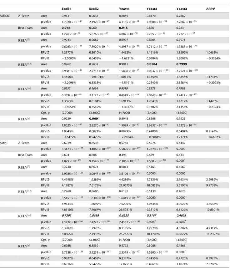
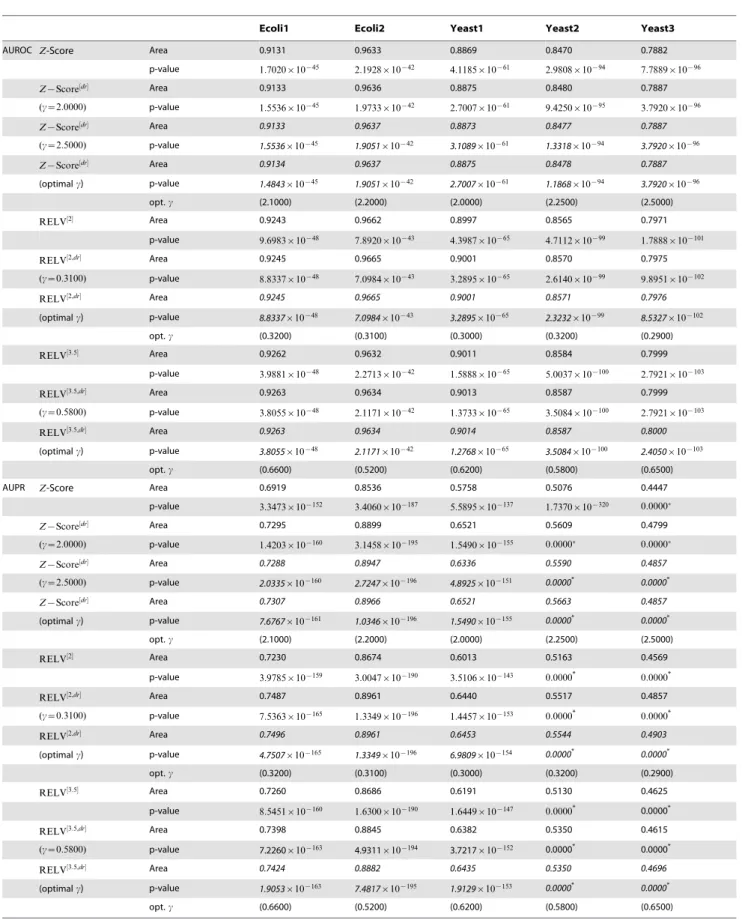
Table 1.Prediction Performances for the DREAM3 Networks.{
Ecoli1 Ecoli2 Yeast1 Yeast2 Yeast3 ARPV
AUROC Z-Score Area 0.9131 0.9633 0.8869 0.8470 0.7882
p-value 1.7020|10{45 2.1928|10{42 4.1185|10{61 2.9808|10{94 7.7889|10{96
Best Team Area 0.948 0.960 0.915 0.856 0.783
p-value 1.226|10{52 5.876|10{42 4.087|10{70 5.755|10{99 1.722|10{92
RELV½2 Area 0.9243 0.9662 0.8997 0.8565 0.7971
p-value 9.6983|10{48 7.8920|10{43 4.3987|10{65 4.7112|10{99 1.7888|10{101
RPV-Z 1.2377% 0.3010% 1.4432% 1.1216% 1.1292% 1.0465%
RPV-B 22.5000% 0.6458% 21.6721% 0.0584% 1.8008% 20.3334%
RELV½3:5 Area 0.9262 0.9632 0.9011 0.8584 0.7999
p-value 3.9881|10{48 2.2713|10{42 1.5888|10{65 5.0037|10{100 2.7921|10{103
RPV-Z 1.4458% 20.0104% 1.6011% 1.3459% 1.4844% 1.1734%
RPV-B 22.2996% 0.3333% 21.5191% 0.2840% 2.1584% 20.2093%
RELV½p Area 0.9252 0.9634 0.9019 0.8572 0.7998
p-value 6.3691|10{48 2.1171|10{42 8.8649|10{66 2.0648|10{99 3.2413|10{103
RPV-Z 1.3363% 0.0104% 1.6913% 1.2043% 1.4717% 1.1428%
RPV-B 22.4051% 0.3542% 21.4317% 0.1402% 2.1456% 20.2394%
Opt.p (2.7000) (3.3000) (4.7000) (2.4000) (3.3000)
RELV½g Area 0.9229 0.9691 0.8948 0.8508 0.7925
p-value 1.8625|10{47 2.8270|10{43 1.5099|10{63 3.6937|10{96 1.5372|10{98
RPV-Z 1.0843% 0.6021% 0.8879% 0.4480% 0.5494% 0.7143%
RPV-B 22.6477% 0.9479% 22.2104% 20.6081% 1.2171% 20.6602%
AUPR Z-Score Area 0.6919 0.8536 0.5758 0.5076 0.4447
p-value 3.3473|10{152 3.4060|10{187 5.5895|10{137 1.7370|10{320 0.0000
Best Team Area 0.694 0.806 0.493 0.469 0.433
p-value 1.029|10{152 9.154|10{177 7.306|10{117 7.580|10{288 0.000*
RELV½2 Area 0.7230 0.8674 0.6013 0.5163 0.4569
p-value 3.9785|10{159 3.0047|10{190 3.5106|10{143 0.0000* 0.0000*
RPV-Z 4.4798% 1.6286% 4.4286% 1.7139% 2.7434% 2.9989%
RPV-B 4.1787% 7.6179% 21.9675% 10.0853% 5.5196% 9.8738%
RELV½3:5 Area 0.7260 0.8686 0.6191 0.5130 0.4625
p-value 8.5451|10{160 1.6300|10{190 1.6449|10{147 0.0000* 0.0000*
RPV-Z 4.9133% 1.7692% 7.5200% 1.0638% 4.0027% 3.8538%
RPV-B 4.6110% 7.7667% 25.5781% 9.3817% 6.8129% 10.8301%
RELV½p Area 0.7293 0.8688 0.6225 0.5167 0.4628
p-value 1.5737|10{160 1.4721|10{190 2.4503|10{148 0.0000* 0.0000*
RPV-Z 5.3902% 1.7926% 8.1105% 1.7928% 4.0702% 4.2312%
RPV-B 5.0865% 7.7916% 26.2677% 10.1706% 6.8822% 11.2397%
Opt.p (2.7000) (3.3000) (4.7000) (2.4000) (3.3000)
RELV½g Area 0.6988 0.8539 0.5772 0.5088 0.4468
p-value 9.7338|10{154 2.9231|10{187 2.5519|10{137 1.5200|10{321 0.0000*
RPV-Z 0.9827% 0.0469% 0.2397% 0.2456% 0.4725% 0.3975%
RPV-B 0.6916% 5.9429% 17.0751% 8.4961% 3.1874% 7.0786%
RPV-Z: relative performance variation with respect to theZ-score based method; RPV-B: relative performance variation with respect to the best team; ARPV: averaged relative performance variation of the 5 networks.
{
RELV½p, which stands for the method with the optimal normalization parameterp, generally can not be applied in actual estimations. The purposes to include its inference results here are only to make it clear that significant estimation performance degradation does not occur when the parameterpdeviates from its optimal value.
*Due to some precision issues of the method suggested by the DREAM project organizers, thesep-values can not be distinguished from zero in actual computations, which makes it impossible to compare scores of the adopted GRN topology estimation methods.
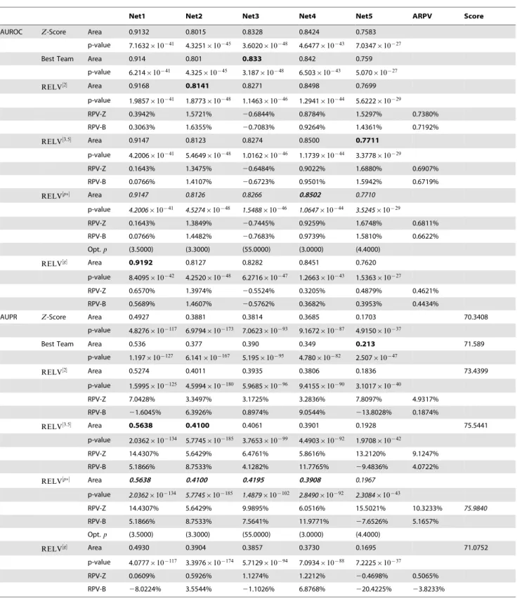
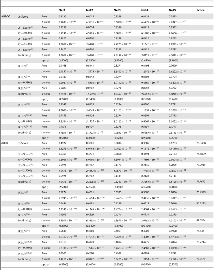
Table 2.Prediction Performances for the DREAM4 Networks.{
Net1 Net2 Net3 Net4 Net5 ARPV Score
AUROC Z-Score Area 0.9132 0.8015 0.8328 0.8424 0.7583
p-value 7.1632|10{41 4.3251|10{45 3.6020|10{48 4.6477|10{43 7.0347|10{27
Best Team Area 0.914 0.801 0.833 0.842 0.759
p-value 6.214|10{41 4.325|10{45 3.187|10{48 6.503|10{43 5.070|10{27
RELV½2 Area 0.9168 0.8141 0.8271 0.8498 0.7699
p-value 1.9857|10{41 1.8773|10{48 1.1463|10{46 1.2941|10{44 5.6222|10{29
RPV-Z 0.3942% 1.5721% 20.6844% 0.8784% 1.5297% 0.7380%
RPV-B 0.3063% 1.6355% 20.7083% 0.9264% 1.4361% 0.7192%
RELV½3:5 Area 0.9147 0.8123 0.8274 0.8500 0.7711
p-value 4.2006|10{41 5.4649|10{48 1.0162|10{46 1.1739|10{44 3.3778|10{29
RPV-Z 0.1643% 1.3475% 20.6484% 0.9022% 1.6880% 0.6907%
RPV-B 0.0766% 1.4107% 20.6723% 0.9501% 1.5942% 0.6719%
RELV½p Area 0.9147 0.8126 0.8266 0.8502 0.7710
p-value 4.2006|10{41 4.5274|10{48 1.5488|10{46 1.0647|10{44 3.5245|10{29
RPV-Z 0.1643% 1.3849% 20.7445% 0.9259% 1.6748% 0.6811%
RPV-B 0.0766% 1.4482% 20.7683% 0.9739% 1.5810% 0.6622%
Opt.p (3.5000) (3.3000) (55.0000) (3.0000) (4.4000)
RELV½g Area 0.9192 0.8127 0.8282 0.8451 0.7620
p-value 8.4095|10{42 4.2520|10{48 6.2716|10{47 1.2663|10{43 1.5363|10{27
RPV-Z 0.6570% 1.3974% 20.5524% 0.3205% 0.4879% 0.4621%
RPV-B 0.5689% 1.4607% 20.5762% 0.3682% 0.3953% 0.4434%
AUPR Z-Score Area 0.4927 0.3881 0.3814 0.3685 0.1703 70.3408
p-value 4.8276|10{117 6.9794|10{173 7.0623|10{93 9.1672|10{87 4.9150|10{37
Best Team Area 0.536 0.377 0.390 0.349 0.213 71.589
p-value 1.197|10{127 6.141|10{167 5.195|10{95 4.780|10{82 2.507|10{47
RELV½2 Area 0.5274 0.4011 0.3935 0.3806 0.1836 73.4399
p-value 1.5995|10{125 4.5994|10{180 5.9685|10{96 9.4155|10{90 3.1017|10{40
RPV-Z 7.0428% 3.3497% 3.1725% 3.2836% 7.8097% 4.9317%
RPV-B 21.6045% 6.3926% 0.8974% 9.0544% 213.8028% 0.1874%
RELV½3:5 Area 0.5638 0.4100 0.4061 0.3901 0.1928 75.5441
p-value 2.0362|10{134 5.7745|10{185 3.7653|10{99 4.4903|10{92 1.9708|10{42
RPV-Z 14.4307% 5.6429% 6.4761% 5.8616% 13.2120% 9.1247%
RPV-B 5.1866% 8.7533% 4.1282% 11.7765% 29.4836% 4.0722%
RELV½p Area 0.5638 0.4100 0.4195 0.3908 0.1967 p-value 2.0362|10{134 5.7745|10{185 1.4879|10{102 2.8490|10{92 2.3084|10{43
RPV-Z 14.4307% 5.6429% 9.9895% 6.0516% 15.5021% 10.3233% 75.9840
RPV-B 5.1866% 8.7533% 7.5641% 11.9771% 27.6526% 5.1657%
Opt.p (3.5000) (3.3000) (55.0000) (3.0000) (4.4000)
RELV½g Area 0.4930 0.3904 0.3857 0.3730 0.1695 71.0752
p-value 4.0777|10{117 3.3976|10{174 5.7129|10{94 7.0934|10{88 7.2225|10{37
RPV-Z 0.0609% 0.5926% 1.1274% 1.2212% 20.4698% 0.5065%
RPV-B 28.0224% 3.5544% 21.1026% 6.8768% 220.4225% 23.8233%
RPV-Z: relative performance variation with respect to theZ-score based method; RPV-B: relative performance variation with respect to the best team; ARPV: averaged relative performance variation of the 5 networks.
{
The purposes to include the inference results ofRELV½pare completely the same as those of Table 1. That is, to clarify that deviation of the parameterpfrom its optimal value usually does not lead to significant estimation performance degradations.
effective in distinguishing direct and indirect regulations, and therefore reducing the so-called cascade errors in GRN topology inference.
In addition, compared with the best team of DREAM3, although the AUROC specification has become slightly worse for some networks, bothRELV½2andRELV½3:5show improvement in the AUPR specification for every network, and the biggest
improvement is greater than 20%. In comparison with the best
team of DREAM4, although these two methods occasionally show some great performance decrements, for example, the AUPR specification ofRELV½2for the Net5 network is about14%lower than that of the best team, they still yield better results on average in both AUROC and AUPR specifications. According to the report in the web site of the DREAM project for the Size 100
subchallenges of DREAM3, thep{value of the AUPR
specifica-tion corresponding to the Yeast3 network of the best team is very close to0and its score can not be calculated due to some precision difficulties [16]. This has been confirmed by the results reported in
Table 1, in which several computed p-values are zero that is
impossible in practice. As the AUPR specifications of RELV½2,
RELV½3:5, RELV½p and RELV½g with that network are all
higher than that of the best team, the corresponding scores of these estimators can not be computed, either. For the DREAM4 subchallenges, based on the evaluation scripts provided by the DREAM project organizers, the score of the suggested method is computed for every adopted normalization which is also included in Table 2. These results make it clear that both RELV½2 and RELV½3:5 could have ranked the first place in the Size 100 subchallenges of DREAM3 and DREAM4. But it should be emphasized that these comparisons are only of some reference values, noting that all the participants of the DREAM project were completely blind to both the structure and the dynamics of the networks.
Concerning the subchallenges of DREAM4, note that the best
team integrated their down ranking method with the Z-score
based method, and the score improvement does not exceed
1:3point. On the other hand, the scores of the methodsRELV½2
and RELV½3:5 are respectively greater than this best team approximately 1:8points and 4:0points. These performance improvements appear not to be a small one. When the average ratio is considered for the subchallenges of DREAM3 about the improvements on the AUROC and the AUPR specifications, similar conclusions can also be achieved.
Whenp-values are directly used in comparing performances of these estimation algorithms, consistent conclusions can be
achieved. For example, when the p-value of the AUPR
specification is taken into account for the Net1 network of
DREAM4, the values of theZ-score based method and the best
team are respectively about2:3709|1017times and5:8786|106 times of that of the methodRELV½3:5.
It appears also worthwhile to note that the best team of DREAM4 utilized an estimation method different from that
adopted by the best team of DREAM3. The results of Tables 1 and 2 may imply that the method suggested in this paper shares advantages of different approaches, and overcomes to some extent their disadvantages. But a theoretically solid justification for this declaration is still under investigation, and further efforts are required to clarify the actual reasons behind these phenomena.
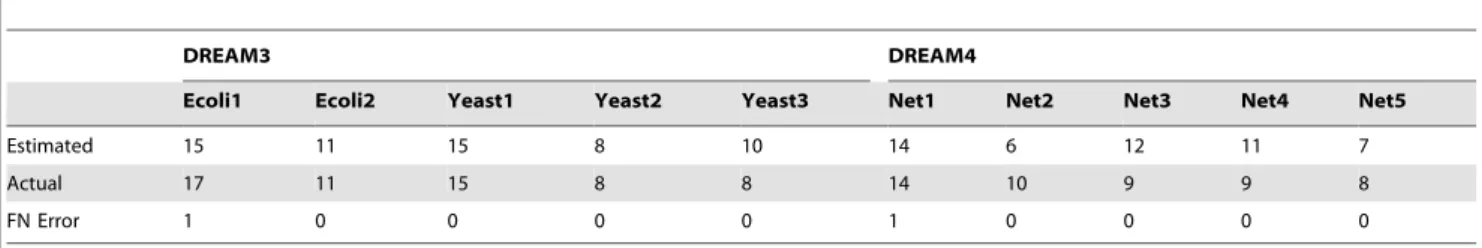
Note that in the estimation algorithm suggested in this paper, the step of estimating genes with a zero in-degree plays an important role. To see the effectiveness of the proposed method in this estimation, the number of genes estimated to be of a zero in-degree is given in Table 3 for each network of DREAM3 and DREAM4, together with its actual value. In this estimation,l2,
Pmin and Pmax are selected as the same as those adopted in
obtaining the estimation results reported in Tables 1 and 2. In this table, an estimation error has also been given which stands for the number of genes that can be regulated by other genes but are estimated to be with a zero in-degree, which is called in this paper, with a slight abuse of terminology, also as a FN (false negative) error.
Table 3 shows that the suggested method is really effective in estimating genes that can not be regulated by other genes. More detailed analyzes on the estimation results show that if an FN error occurs, then, the genes that are wrongly estimated to be of a zero in-degree are usually regulated by less than 2 other genes. Moreover, if a gene with a zero in-degree is wrongly estimated to be regulated by other genes, then, in the corresponding probabilities, say,Pjis, the number of values that are significantly
greater than 0 is usually less than 2. These types of mistakes appear reasonable in GRN topology estimation, noting that a large scale GRN usually has a sparse structure and measurement errors may happen to make the estimated value for every RELV of a gene with a small in-degree indistinguishable from0. On the contrary, measurement errors are also able to make a few estimated RELVs of a gene with a zero in-degree significantly different from0.
Robustness of the Suggested Method
Recall that in the suggested GRN topology estimation algorithm, parametersl1,l2, PminandPmax should be selected.
While these parameters have some biological interpretations, their selection has not been completely settled from a theoretical viewpoint. It is therefore interesting to investigate how sensitive the estimation accuracy is to the variation of these parameters. As knockout experimental data is used, it appears reasonable to selectl2asl2~0:5. On the other hand,Pmin~0:0005=0:05and
Pmax~0:2also seem to be an appropriate choice, as a big relative
change with a smallPmin does not result in a significantly large
Piimz1, and a greatPmaxmay lead to a large amount of mistakes of
wrongly estimating a gene regulated by other genes as a gene with a zero in-degree. These arguments imply that in GRN
topology estimation, selection of the parameter l1 is more
essential.
Table 3.Estimated Number of Genes with a Zero In-degree.
DREAM3 DREAM4
Ecoli1 Ecoli2 Yeast1 Yeast2 Yeast3 Net1 Net2 Net3 Net4 Net5
Estimated 15 11 15 8 10 14 6 12 11 7
Actual 17 11 15 8 8 14 10 9 9 8
FN Error 1 0 0 0 0 1 0 0 0 0
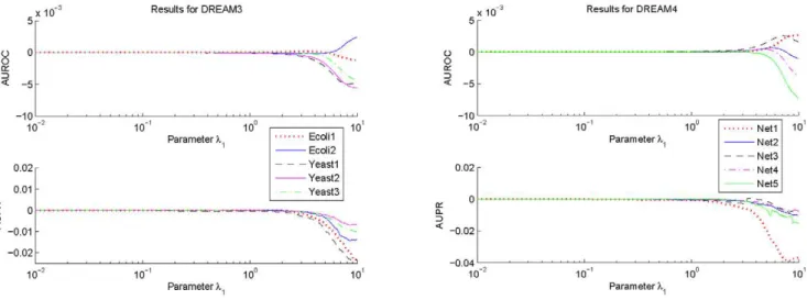
To investigate influences of the parameterl1on the prediction
accuracy of GRN topology inference,100samples are taken for
this parameter which is logarithmically equally spaced over the interval ½10{2, 10. For every sampled parameter l
1, values of AUROC and AUPR for each network of DREAM3 and DREAM4 are calculated with the suggested estimation algorithm using respectively the 2-norm and the 3:5-norm based normali-zations. The difference between the obtained AUROC specifica-tion and that withl1~0:01, as well as the difference between the obtained AUPR specification and that withl1~0:01, are shown in Figures 1 and 2. In these calculations,l2, Pmin and Pmax are
respectively fixed to be the same values as those used before. From Figures 1 and 2, it can be seen that performances of the
proposed algorithm do vary with the parameter l1. But these
performances keep almost the same values if l1[½0:01,1. Moreover, except a few networks, these performances begin to decrease from l1~1. Consistent observations have also been
found for the suggested inference algorithm with other p-norm
based and the geometric average based normalizations. These
results imply that in practical applications, it may not be very difficult to select an appropriatel1. In this paper, this parameter is usually chosen as0:01.
To understand influences of different normalizations on GRN topology estimation accuracy, variations of the AUROC and
AUPR specifications with the parameter p have also been
investigated. The results are given in Figure 3. Note that in this
figure, the parameterpfor the Net3 network of DREAM4 should
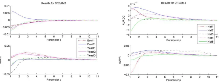
be modified. Its variation interval for this network is½1, 101. Once again, to make the variations clearer, some particular values have been extracted from the calculated AUROC and AUPR specifications, which are given in detail in the caption of the figure. In these calculations, the parametersl1,l2,PminandPmax
are chosen as the same as those adopted before.
From Figure 3, it is clear that the adopted estimation accuracy
metrics indeed vary with the parameter p. The optimal p that
maximizes the AUROC specification is different from that maximizes the AUPR specification, and different network has a different optimalp. On the other hand, it is also clear from this
Figure 1. Variations of the AUROC and AUPR specifications ofRELV½2as a function of the parameterl
1.To make the variations clearer,
this figure only shows the deviations of the AUROC and the AUPR specifications with the sampledl1from those withl1~0:01.
doi:10.1371/journal.pone.0031194.g001
Figure 2. Variations of the AUROC and AUPR specifications ofRELV½3:5 as a function of the parameterl
1.To make the variations
clearer, this figure only shows the deviations of the AUROC and the AUPR specifications with the sampledl1from those withl1~0:01.
figure that although the optimalpis different for each network and each specification, significant specification change does not arise when the parameterpvaries over a relatively large interval. More specifically, for each network, the variation of the AUROC specification is not larger than 0.01 in magnitude, and whenp§2, the variation of the AUPR specification is not larger than 0.03 in magnitude. For some particular networks, such as Ecoli2, Yeast3 and Net4, the variation magnitude is much smaller. These observations suggest that in actual applications, it is not very
difficult to find a suboptimal value for the parameter p.
Particularly, p~3:5 appears to be an appropriate selection for every network of DREAM3 and DREAM4. This can also be confirmed from the results of Tables 1 and 2, which show that,
compared with the results with the optimal p, significant
performance degradation generally does not arise with the method
RELV½3:5. It is worthwhile to note thatp~3:5is different from those that are widely adopted in system analysis and synthesis, in whichp~1,2, or?is used more extensively [25,27].
On the other hand, to investigate the validity of the suggested technique for estimating genes with a zero in-degree, the obtained
iim is perturbed to beiimzj with j~+1,+2,+3,+4. This may simulate the situation under whichiim is different from its actual
value due to estimation errors in ss^i and xx^½iwt,0, as well as the
imperfectness of the adopted assumptions and numerical integra-tion errors, etc. Through the aforemenintegra-tioned perturbaintegra-tions, the estimated number of genes with a zero in-degree can be changed respectively by +1,+2,+3,+4 with respect to that of the unperturbed one. The obtained results for the methodsRELV½2
andRELV½3:5 are respectively shown in Figures 4 and 5. When other normalizations are utilized, consistent observations have
Figure 3. Variations of the AUROC and AUPR specifications ofRELV½½pwith the increment of the parameterp.The results shown in this figure are as follows. Ecoli1: 0.9276, AUPR-0.7019; Ecoli2: 0.9625, AUPR-0.8665; Yeast1: 0.9026, AUPR-0.6135; Yeast2: 0.8601, AUPR-0.4950; Yeast3: 0.8006, AUPR-0.4561; Net1: 0.9137, AUPR-0.5494; Net2: 0.8089, AUPR-0.3824; Net3: AUROC-0.8265, AUPR-0.3917; Net4: AUROC-0.8474, AUPR-0.3719; Net5: AUROC-0.7705, AUPR-0.1921.{For the Net3 network of DREAM4, the variation interval of the parameterpis½1, 101.
doi:10.1371/journal.pone.0031194.g003
Figure 4. Variations of the AUROC and AUPR specifications ofRELV½½2with perturbations oni
m.To make the variations clearer, only deviations of the AUROC and AUPR specifications from those of the unperturbediimare shown here.
been obtained and the conclusions are similar. To make the variations clearer, once again, only difference is shown between the obtained specifications and those with the estimatediim.
From Figures 4 and 5, it can be seen that estimation performances with some networks can become slightly better
when iim deviates from the value adopted in the suggested
estimation algorithm. For example, both the AUROC and the AUPR specifications of the Ecoli1 network and the Net2 network are better when the gene numberediimz1is also regarded to be of a zero in-degree, and the AUPR specification of the Yeast2 network and the Net5 network is a little higher when the gene numberediimz1is also considered as a gene not regulated by other genes. However, these performance improvements are not very significant, and when all the networks are taken into account, it is still better to useiim in GRN topology estimations. In addition, if
there are small variations iniim, significant performance decrement
usually does not arise.
Performances for Integration of Knockdown and Knockout Data
In this subsection, the suggested method for integrating knockout and knockdown experimental data is applied to the Size 100 subchallenges of both DREAM3 and DREAM 4. As mentioned before, rather than to develop a high performance integration method, the major purposes to include these results are to clarify effectiveness differences of knockout and knockdown experimental data in GRN topology estimations when the suggested method is adopted. In order to compare estimation
performances, results using the Z-score based method are also
integrated with completely the same procedure, that are respectively obtained from the knockout and knockdown exper-imental data.
The computational results of the Size 100 subchallenges of DREAM3 and DREAM4 are given respectively in Tables 4 and 5, in whichKD,KOandMIXstand respectively for the estimation results obtained from knockdown experimental data only, knockout experimental data only and both of them using the above integration algorithm. Due to space considerations, the reported results are restricted to those with respectively the2-norm and 3:5-norm based normalization. When other normalizations are utilized, consistent observations have been obtained and the
conclusions are similar. For comparisons, the results are also included that are obtained using theZ-score based method.
From Tables 4 and 5, it is clear that when applied to the DREAM4 subchallenges, the suggested integration procedure is
able to improve estimation performances for both the Z-score
based method and the estimation algorithm suggested in this paper. As a matter of fact, compared with the results using only knockout experimental data, although there is one network with which the AUPR specification has been slightly degraded when the methodRELV½3:5 is used, the final score ofRELV½3:5 has been increased by about 3.8 points. Furthermore, the scores of the
method RELV½2 and the Z-score based method have been
increased more significantly, which are respectively about 5.6 and 7.0 points. These improvements seem not small, noting that the
best team of DREAM4 integrated theZ-score based method with
their down ranking method, but the obtained merits are less than 1.3 points. In addition, this integration method appears more effective for theZ-score based method. More specifically, under such a situation, for each network, every adopted specification has been improved, and the final score has been increased almost
10%. These observations are significantly different from those of [18–20], which indicated that when knockout experimental data are available, knockdown experimental data is of little values in GRN topology inference.
Similar conclusions can be achieved if the p-values of the
obtained estimation specifications are directly compared. However, when utilized in the DREAM3 subchallenges, the aforementioned integration procedure does not work very well
either with the Z-score based estimation algorithm or the
algorithm suggested in this paper. Compared with the results using only knockout experimental data, this integration even worsen almost every specification of each network. The reasons are still not clear which are worthy of further efforts. But from these observations, it is clear that compared with those of DREAM3, information in the data sets of DREAM4 about the structure of a GRN are more consistent which are respectively contained in the knockout and knockdown experimental data.
Note that although in DREAM3, only measurement errors are added into the simulated experimental data, variances of the measurement errors are assumed to be of the same value for every gene under all situations, no matter it is in the wild type, or when
Figure 5. Variations of the AUROC and AUPR specifications ofRELV½½3:5with perturbations onim.To make the variations clearer, only deviations of the AUROC and AUPR specifications from those of the unperturbediimare shown here.