A META-ANALYSIS ON THE BANK OF JAPAN QUANTITATIVE EASING POLICY: THE BANK OF JAPAN’S EFFECTIVENESS TO PROMOTE ECONOMIC
GROWTH
Pedro André Simões Roque Linhares
Dissertation submitted as partial requirement for the conferral of
Master in Economics
Supervisor:
Prof. Alexandra Ferreira-Lopes, Assistant Professor, ISCTE Business School, Economics Department
Co-supervisor:
Prof. Tiago Miguel Guterres Neves Sequeira, Associate Professor, Universidade da Beira Interior, Management and Economics Department
– Spine – A MET A -AN ALY S IS O N TH E BANK OF JAP A N Q UA NT IT ATI V E EA S IN G POLI C Y: TH E B AN K O F JAPAN’ S EFF ECTIV ENE S S TO PR OMO TE E C ON OMI C GROW TH
P
edro
A
ndré S
im
õ
es
R
o
que L
inh
a
re
s
III Abstract
As the Qualitative and Quantitative Easing programmes are still in place there have been signs that the Japanese economy will maintain a path of moderate economic growth, still, without glancing the desired 2% inflation. The question over whether and how the Bank of Japan successive quantitative easing programmes, which were based on an unprecedented increase on the central bank’s asset sheet, have been successful in promoting a steady growth of the Japanese Economy, has been debated by the literature that is focused on the transmission channels of monetary policy. We present a comprehensive meta-analysis that focus on the literature that have been studying the effectiveness of the Bank of Japan’s policies during the 2001 to 2016 period, that resorts to the Vector Auto-regressive methodology to analyze, through impulse response functions, how monetary policy shocks impact output. An analysis based on funnel plots – Funnel Asymmetry Test – and linear regressions – Precision Effect Test – does not provide evidence of publication bias, neither the consensus over the output growth during the quantitative years. A meta-probit analysis suggests that a study with the characteristics mentioned above, which uses certain variables to build the model – industrial output, price level, bond yield and either the money base or the money supply – as well as different specifications in the data used – increasing the number of observations used or choosing quarterly data – will affect the probability of reporting statistically significant output growth; notwithstanding, the evidence found in this last analysis varies in terms of statistical robustness.
Keywords: Quantitative easing, Bank of Japan, Effects of monetary policy on economic growth
IV Resumo
Ainda com o programa de Qualitative e Quantitative Easing em vigor, têm existido sinais de que a economia japonesa manterá um caminho de moderada recuperação económica; não obstante, sem se vislumbrar o desejado crescimento da inflação a 2%. A questão em torno de se, e como, os sucessivos programas de quantitative easing baseados num crescimento sem precedentes dos ativos do Banco Central do Japão, têm tido sucesso em promover o crescimento estável da economia japonesa, tem sido discutida na literatura que se foca nos mecanismos de transmissão da política monetária. Neste estudo, apresentamos uma meta-análise que se foca na literatura que estuda a eficácia das políticas do Banco do Japão durante o período de 2001 a 2016. Literatura essa que recorre a metodologia baseada em modelos Vector Auto-regressive, para analisar através de funções de resposta a impulso, como é que os choques causados por ferramentas de política monetária afetam a produção da economia japonesa. Com base numa análise em gráficos de dispersão em funil – Funnel Asymmetry Test – e em regressões lineares – Precision Effect Test – não obtivemos provas que sugerissem publication bias – enviesamento dos resultados publicados em revistas – nem provas que sugerissem um consenso entre a literatura visada, relativamente ao valor do crescimento da atividade económica no Japão durante os períodos de quantitative easing. Uma análise baseada em modelos meta-probit, sugere que a inclusão, em estudos com a estrutura atrás mencionada, de certas variáveis no modelo a estimar (relativas à economia Japonesa) – o output industrial, o nível dos preços, as taxas de retorno de títulos da dívida japonesa, ou tanto a base monetária como a oferta de moeda nacional – tal como outras especificações relativas ao tipo de dados utilizados – o incremento do número de observações ou a utilização de dados trimestrais – podem afetar a probabilidade das estimações virem a reportar um crescimento positivo e estatisticamente significativo na atividade económica. Os resultados encontrados nesta última análise variam em termos de robustez estatística.
Keywords: Quantitative easing, Banco Central do Japão, Efeitos da política monetária no crescimento económico
V Acknowledgements
A particular acknowledgement of my gratitude to Professor Alexandra Ferreira Lopes and Professor Luís Martins for the time and the patience.
VI Table of Contents ABSTRACT ... III RESUMO ... IV ACKNOWLEDGEMENTS ... V TABLE OF CONTENTS ... VI LIST OF ACRONYMS ... VII LIST OF FIGURES ... X LIST OF TABLES ... X
1. INTRODUCTION ... 1
2. THE CONTEXT OF THE STUDY: REVIEWING THE JAPANESE CASE AND THE LITERATURE ON META-ANALYSIS ... 2
2.1 THE EVOLUTION OF THE JAPANESE ECONOMY AND THE NEED FOR UNCONVENTIONAL MONETARY POLICIES... 2
2.2 MONETARY POLICY TRANSMISSION UNDER META-ANALYSIS ... 3
3. DATA AND METHODOLOGY ... 6
3.1 METHODOLOGY -CONSTRUCTION OF THE DATABASE ... 7
3.2 DESCRIPTION OF THE DATABASE ... 8
3.2.1 Authorial Information ... 9
3.2.2 Data ... 10
3.2.3 Methodological Specifications ... 11
3.2.4 Estimates ... 19
4. DESCRIPTIVE STATISTICS... 27
5. PUBLICATION BIAS SCREENING ... 33
5.1 FUNNEL ASYMMETRY TEST ... 35
5.2 PRECISION EFFECT TEST ... 40
5.3 ESTIMATION RESULTS ... 42
6. META-PROBIT ESTIMATION ... 46
6.1 FURTHER VARIABLE TREATMENT ... 47
6.2 THE PROBIT MODEL AND PRELIMINARY PROCEDURES ... 51
6.3 STEPWISE VARIABLE SELECTION ANALYSIS OF THE PROBIT MODEL... 57
6.4 ADJUSTED PREDICTIONS AND MARGINAL EFFECTS ... 63
6.5 HETEROSCEDASTICITY ANALYSIS ... 67
6.6 INTERACTION EFFECTS ... 69
6.7 DISCUSSION OF SOME METHODOLOGICAL CHOICES ... 71
7. CONCLUSION ... 73
8. BIBLIOGRAPHY ... 76
9. ANNEX I ... 79
10. ANNEX II ... 101
VII List of Acronyms
3MIR – 3-month interest rate AME – Average Marginal Effects
AOAB – Average Outstanding Account Balance APP – Asset Purchase Program
BBS – Bank Balance Sheets
BMA – Bayesian Model Averaging BoJ – Bank of Japan
BOJPGB – Bank of Japan Purchase of Government Bonds BOJSP – Bank of Japan Stock Purchases
BVAR – Bayesian Vector Auto-regressive CAB – Current Account Balance
CCIG – Core CPI inflation Gap CCPI – Core Consumer Price Index CDF – Cumulative Distribution Function CEC – Credit Easing Channel
CGPI – Corporate Good Price Index CI – Confidence Intervals
CME – Comprehensive Monetary Easing CPI – Consumer Price Index
CR – Call Rate
DEIT – Direct Effect of Inflation Targeting ETF – Exchange Trade Fund
FAT – Funnel Asymmetry Test
FAVAR – Factor Augmented Vector Auto-regressive FG – Forward Guidance
FIRSTDIF – First Differences GDP – Gross Domestic Product GDPD – GDP deflator
GJ – General Journal
HP filter –Hodrick–Prescott filter ICC – Intra-class Correlation
VIII
IER – Increase in the Excess Reserves Int. Obs – Intervals of Observations IO – Industrial Output
IOBOJMP – Indirect Observance of Bank of Japan Monetary Policy IR – Inflation Rate
IRF – Impulse Response Function IRR – Interest Rate of Reference IT – Information Technologies JGB – Japanese Government Bond
J-REITS – Japanese Real Estate Investment Trust LR – Likelihood Ratio
LTM – Latent Threshold Model LVS – Levels
MB – Monetary Base MJ – Monetary Journal
MLE – Maximum Likelihood Estimation MLME – Multilevel Mixed Effect MP – Monetary Policy
MPP – Monetary Policy Proxy MS – Money Supply
MS-FAVAR– Markov Switching Factor Augmented Vector Auto-regressive MSt – Money Stock
MSVAR – Markov Switching Vector Auto-regressive MV – Money Variable
NA – Non-Available
NEER – Nominal Effective Exchange Rate NS – Non-Significant
NYDSR – Nominal Yen/Dollar Spot Rate Obs – Observations
OG – Output Gap
OLS – Ordinary Least Squares OTF – Other Timeframes OTS – Other Type of Shocks
IX
PCI – Percentile Confidence Intervals PET – Precision Effect Test
PL – Price Level PP – Published Paper
PRE – Portfolio Re-balancing Effect QE – Quantitative Easing
QQE – Qualitative Quantitative Easing REER – Real Effective Exchange Rate RIRC – Real Interest Rate Channel RR – Repo Rate
S10YCR – Difference between the 10-year JGB yield and the Call Rate S5YCR – Difference between the 5-year JGB yield and the Call Rate SD – Standard Deviation
SE – Standard Error
SMB – Shock to the Monetary Base SMS – Shock to the Money Stock SP – Stock Prices or Stock Price Index SPC – Stock Price Channel
SSTIRR – Shock to the Short-term Interest Rate of Reference SVAR – Structural Vector Auto-regressive
TBBR – Total Bank Balance Reserves TCU – Transmission Channel Undefined TQE – Tobin's Q Effect
TVP-VAR – Time-Varying Parameter Vector Auto-regressive
TWREFER – Trade Weighted Real Effective Foreign Exchange Rate UNIVARA – Univariate Analysis
UR – Unemployment Rate VAR – Vector Auto-regressive VEC – Vector Error Correction WE – Wealth Effect
WP – Working Paper
X List of Figures
Figure 4-a: Overall Effect of the Shock in the Output by Year of Publication/Release
(104 Observations) ... 31
Figure 4-b: Density of Intervals of Maximum Magnitude of the Output Response to a QE Shock or Other Shock ... 32
Figure 4-c: Persistence of the Shock’s Impact in the Output Variable during a Statically Significant Period (in Months; 33 Obs.) ... 33
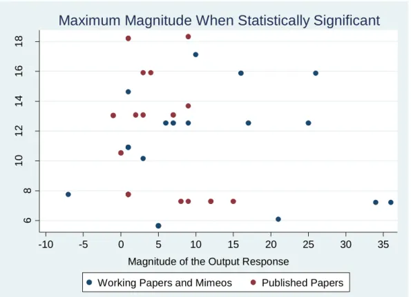
Figure 5-a: Effect-sizes collected from the Literature Selection – Maximum Magnitude ... 38
Figure 5-b: Effect-sizes collected from the Literature Selection – First Quarter ... 39
Figure 5-c: Effect-sizes collected from the Literature Selection – Twelfth Month... 39
Figure 5-d: Effect-sizes collected from the Literature Selection – Twenty-fourth Month ... 40
Figure 9-a: Effect Sizes by Year of Publication/Release (104 Obs.) ... 100
Figure 9-b: Density of Intervals of Maximum Magnitude of the Output Response to a Non-QE Shock ... 100
Figure 9-c: Persistence of the Shock’s Impact in the Output Variable during a Statically Significant Period (in Months; 8 Obs.) ... 101
Figure 11-a: Interaction QE*Bond, Significance and Corrected Effect Respectively. 109 Figure 11-b: Interaction IO*Price, Significance and Corrected Effect Respectively... 110
Figure 11-c: Interaction IO*Bond, Significance and Corrected Effect Respectively. . 109
Figure 11-d: Interaction QE*Bond, Significance and Corrected Effect Respectively. 110 List of Tables Table 2-1: Effect Sizes used by Meta-analysis Studies on Monetary Policy Transmission Mechanisms and the Countries or Regions that were considered in the respective Literature Selection... 4
Table 3-1: Resume of the Information Collected to Build the Database... 9
Table 3-2: Types of VAR Methodology found in the Literature by Categories ... 12
Table 3-3: List of Variables that Compose the Models Reported in the Literature ... 13
Table 3-4: Type of Shocks found in the Literature Selection and how they were grouped ... 17
Table 3-5: The code of the overall effect of the monetary policy shock in output (Signal of the shock's impact in the output variable) ... 21
Table 3-6: IRFs Magnitude – Intervals of values ... 23
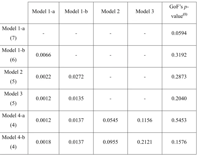
Table 5-1: Main PET Results ... 45
Table 6-1: New Variables and Re-categorized Variables for Probit Estimation ... 49
Table 6-2: P-values of the Coefficient's Z-statistic taken from Univariate Probit Models ... 54
XI
Table 6-3: Meta-probit Estimation Results ... 60
Table 6-4: Adjusted Prediction of the Outcome Variable for Different values of Obs and Int. Obs ... 64
Table 6-5: Average Marginal Effects ... 67
Table 6-6: Likelihood Ratio Test Chi-square p-values ... 72
Table 9-1: Chronology of the Main Guidelines and Events that Characterize the Acting of Japanese Policy Makers in the Last 18 Years ... 79
Table 9-2: Descriptive Statistics ... 81
Table 9-3: Descriptive Statistics for the Estimates – Persistence and Magnitude, Discriminating between QE and Non-QE shocks ... 97
Table 9-4: Percentage Distribution of the Variations in the VAR Family Identified in the Literature Selection (104 Obs.) ... 98
Table 9-5: Explicit Reference to Transmission Mechanisms ... 99
Table 10-1: PET Results for Maximum Magnitude Effect-Sizes ... 101
Table 10-2: PET Results for 1st Quarter Effect-Sizes ... 102
Table 10-3: PET Results for 12th Month Effect-Sizes ... 104
Table 10-4: PET Results for 24th Month Effect-Sizes ... 105
Table 11-1: Correlation Matrix of the Variables used in the Univariate Analysis ... 106
1 1. Introduction
The Bank of Japan has been employing measures of unconventional monetary policy for over 15 years now. A substantial empirical bulk of work has appeared since then on the effects of the measures of unconventional monetary policy on several fundamental variables of the Japanese economy. These measures were set in place, specially, to stimulate the anemic Japanese economy. However, the Japanese case is still perceived by the majority of the audience – policy makers, researchers, investors, or even the public in general – as one of the most notorious histories of an economy incapable of detaching itself from stagnation, regardless of the efforts in the opposite direction. In the following study it is analyzed the unconventional monetary policy of the Bank of Japan (BoJ) and its impact on the economic growth of the Japanese economy. Specifically, relying upon meta-analysis to withdraw valid and statistically relevant conclusions based on a selection of empirical literature that assesses and measures the impact of the behavior of the Bank of Japan in the Japanese economic activity, with particular emphasis on GDP and/or its growth.
This study has the following structure: Section 2 establishes the context of the study in regards to the Japanese case and introduces previous cases of meta-analysis literature, which focused on monetary policy transmission. Section 3 gives an account on how data has been collected from the literature on Japanese Monetary Policy, and how has been treated and organized. Section 4 presents descriptive statistics based on the dataset built and described in Section 3, giving an account on some key elements regarding the conclusions and estimations reported in that very same literature. Section 5 makes use of the same dataset to conduct a type of analysis based on funnel plots and linear regressions, to screen for biased results in the published literature here addressed. Section 6 presents a series of probit estimations that try to unveil whether the choice or presence of certain elements that characterize that same literature, regarding the type of data used, or other methodological aspects, are able to predict what they report.
2 2. The Context of the Study: Reviewing the Japanese Case and the Literature on
Meta-analysis
5.1 The Evolution of the Japanese Economy and the Need for Unconventional Monetary Policies
The last 15 years of the Japanese economy can be described as a row of successive attempts to recover from the generally designated Japan’s lost decade, the 1990’s. This decade is considered a significant turning point for the Japanese economy, characterized by a long-lasting recession, which ended, in the beginning of the 2000’s, in a combination of negative output gap (as well as sluggish economic growth) and moderate deflation. The prospects for the Japanese economy were many times clouded by the repercussions of internal financial crisis that stroke the economy over time: in the end of the 80’s with the burst of the real estate bubble which contaminated all the financial system; the IT bubble that went bust in 2000; and more recently, the international financial crisis of 2008.
The efforts to revert the scenario persisted throughout the recent economic history of Japan, considered one of the greatest challenges for national policy makers, with special responsibilities for the institution that runs Japan’s monetary policy, the BoJ. In order to revert the scenario of the 90’s, the BoJ engaged in what was known to date to be an unconventional type of policy framework, substituting the main policy tools and the policy targets. The period that fall under this unconventional monetary policy approach, was designated as Quantitative Easing (QE). Since 2001 there have been three programmes that fall under the category of QE, being the last of the programmes implemented (and still in place), designated as the Qualitative and Quantitative Easing (QQE) programme1. There are several features in these programmes that may be pointed out as basic elements that form their identity. The first feature is the fact that this policy framework is called a programme: a conditional set of policy measures, for which pre-established rules determine their continuity or cessation. Adding to this point is the fact that a so called programme implies a sense of closure and goal achievement. This is an attempt by the BoJ to let know private agents of a more active intervention in the economic scenario; in opposition to a later accommodative stance during the 1990’s. Finally, another feature that may be pointed out is the transition for more active
3
operating mechanisms of monetary policy (MP), in opposition to the traditional policy tool, the overnight call rate2. Regarding the overnight call rate, the BoJ maintained what is called the Zero Interest Rate Policy (ZIRP) during the QE years3, until it announced in late January 2016, for the first time, that the level of the call rate would be set at 0.1% below zero4.
Using the definition of Ugai (2015), a QE programme can be seen as the work of two mechanisms that operate through both sides of a central bank’s balance sheet (in this case the BoJ’s). According to the author, if a central bank operates through the purchase of risky assets in order to diminish the imbalances of the financial markets, then the central bank is using the asset side of its balance sheet; if the central bank engages in large-scale operations of government bond purchasing, which will force the monetary base of the economy to expand in a first stage, then is the liability side of the same balance sheet that is being used.
5.2 Monetary Policy Transmission under Meta-Analysis
In what regards the existing literature that could serve as a methodological object of comparison, one could only find a small number of studies that employ meta-analysis focusing on monetary policy transmission; and more specifically, that simultaneously distinguishes between types of VAR methodologies employed, and made use of an effect size based on impulse response functions5 (IRFs). Notwithstanding, Table 2-1 resumes some of the existing literature addressed to other countries. For instance, Grauwe and Storti (2004) used a meta-regression to infer on the factors that could justify the variation of results reported in the literature, regarding the impacts of monetary policy shocks in the output and the price level. The same meta-analysis points out a large variation in the results reported in the literature, concerning the estimations for output; stating as well that part of that variation could be explained by whether the
2The call rate is the designated reference interest rate of the BoJ; an overnight interest rate that the BoJ
uses in interbank operations.
3 The ZIRP – when the overnight call rate was set between 1 and 0% – coincided with the QE frameworks
during the periods of 2001 to 2006 and 2010 to 2016.
4 Such novelty in the BoJ’s monetary policy framework is not contemplated in any of the studies selected.
5 The cited studies also used meta-analysis in order to unveil cross-country heterogeneity of results, which
methodologically speaking, leads them to include in their regressions variables that distinguish estimates per country. These variables are based on economic features such has openness to foreign-trade or proxies for financial development. Regardless, our main purpose with this short review was only to stress some of the findings that relate the heterogeneity of the reported results with differences in approaches of the methodology.
4
authors used VAR or SVAR techniques. In a similar fashion, Ridhwan et al. (2010) conducted a meta-analysis, which reported an accentuated variance of estimated output effects taken from the literature; both regarding the speed and magnitude of transmission.
Pitzel and Uusküla (2007) found some evidence, for countries within the EU-15, that higher financial depth is positively correlated with a stronger transmission of monetary shocks. These authors took three exterior variables that measure financial depth for each country, and assessed their correlation with the corresponding monetary shock impacts on output and prices, based on the IRFs reported in the literature. Rusnak et al. (2013) employed a mixed-effects multilevel model, which aimed to capture the reasons behind the price puzzle patterns found across the literature. The findings in this study suggest that, often, patterns observed in the empirical estimates are not consonant with what the theory postulates; the authors also suggest that more observations exert a positive effect on the long-term estimates of the price level after a shock in the interest rate of reference (monetary policy tool), i.e. the price puzzle does not fade with time; and that the reported estimations do vary depending on the VAR specification and output proxy used.
Instead of employing a regression in their research, Havranek and Rusnak (2013) opted for a Bayesian model averaging (BMA) method, in order to withdraw conclusions on the speed of monetary transmission. The authors found that a “best-practice” model based on the results reported by their BMA approach shortens the average time of shock transmission in the price level considerably, when compared with the average taken from the literature results. Moreover, these authors also found that data and methodology factors play a role in explaining the variation of results within the literature. Studies that use monthly data and report strictly decreasing impulse responses are prone to make evidence of a slower transmission; whereas studies that report hump-shaped impulse responses tend to report a faster transmission of monetary policy shocks into the price level.
Table 2-1: Effect Sizes used by Meta-analysis Studies on Monetary Policy Transmission Mechanisms and the Countries or Regions that were considered in the respective Literature
Selection
5
Grauwe and Storti (2004) 1% increase of the interest rate in the output and the price level, caught at the 1st and 5th year.
Austria, Belgium, Denmark, Emerging Countries, Eurozone, Finland, France Germany, Greece, Ireland, Italy, Japan, Luxembourg, Netherlands, Portugal, Spain, Sweden, UK, US.
Pitzel and Uusküla (2007) Maximum level attained by the monetary policy shock in output and price level.
EU-15 countries.
Ridhwan et al. (2010) 1% increase of the interest rate in the output caught at the 14th and 16th quarters and at the maximum and minimum level.
USA, Eurozone and European Union (Non-Eurozone).
Rusnak et al. (2013) 1% increase in the interest rate and in the price level caught at the 3rd, 6th 12th, 18th, and 36th month, plus at the maximum and minimum levels.
Australia, Brazil, Bulgaria, Canada, Czech Republic, Denmark, Estonia, Euro Area, Finland, France, Germany, Greece, Hungary, Ireland, Italy, Japan, Korea, Latvia, Lithuania, Malaysia, New Zealand, Philippines, Poland, Romania,
Slovakia, Slovenia, Spain, Thailand, Turkey, UK, US.
Havranek and Rusnak 1% increase of the interest rate on price level caught at
6
(2013) the minimum level (after
reaching its maximum) for humped-shape responses, and also at the last period available for strictly decreasing responses.
2013)
3. Data and Methodology
A two-stage process was applied to create a pool of studies, which begun with the search for all the studies available in Google Scholar, RePEC, B-on, and Scopus, possessing the following features:
- Attempted to respond to the question whether the Japanese Monetary Policy was effective in promoting economic growth during the QE periods, even if this was not the main question.
- Made use of Vector Auto-regressive (VAR) methodology (or related methodologies).
- And the methodological framework supported their statistical results with the use of impulse response functions (IRFs).
By imposing these features to every study selected, we account for a certain degree of homogeneity within that pool, thus creating the necessary basis for comparability between studies. As an additional criterion, regarding the impulse responses functions, these must account for a shock caused by a monetary policy tool that conveys its impact onto an output proxy. The graphical representations of these impulse responses are the source from which was possible to extract several important features about the literature on the given subject, e.g.: are the monetary policy shocks affecting positively or negatively the Japanese economy?, what is the magnitude and duration of such impacts?, can the authors identify transmission channels through which those impacts are conveyed?, what can one say about the statistical robustness of these IRFs?
Having these features in mind, several combinations of the following set of words were typed in the mentioned search engines: “Japan”; “Economic Growth”; “Output”; “VAR”; “Effect”; “Effectiveness”; “Impact”; “Impulse Response”; “Monetary Policy”;
7
“Quantitative Easing”; “Transmission Channels”; “Transmission Mechanisms”; “Zero Interest Rate Policy”; and “Zero Lower Bound”. The second and much more successful moment of the search process was snowballing from the results found in the first moment6. The search was conducted between March and May 2016.
The data was collected from 30 studies7, registering a total amount of 104 impulse response estimations, covering a publishing period from 2006 to 2016, being the most recent publications considered preferably, since the length of the QE programmes covered were bigger. One criterion settled was that in order to be eligible, a study should include in its period of analysis roughly one year of quantitative easing. A direct consequence of this was to exclude studies or estimates based in periods of analysis before 2002. Aside from this, it was further decided that there would not be a prior exclusion of studies based on their publication characteristics such as their status – the prior expectation that for whatever reason, e.g., the reputation of the author(s) or the journal in which the study is published, might be a source of prior discrimination in the meta-analysis, by distributing more weight to the reported estimations perceived to be more trustable/reliable – or impact – the attempt to quantify that status, e.g., a study’s number of citations within a given period. Despite of not having considered initially these two elements, a treatment of this nature will be given and described in Section 6.
3.1 Methodology - Construction of the Database
Each entry in the database corresponds to a single set of information which intends to register fundamental characteristics of an impulse response of the output variable to a disturbance in a given monetary policy variable. With this database, we intended to register all occurrences of this type in the literature selection here presented. Because, often, the information reported in impulse response functions is not quantified and summarized in a systematic manner, one had to withdraw it from the graphical
6 Snowballing is to continuously look for the citations found in studies that are, or may be important, and
to go look into the cited papers to search for what studies they have cited. Reverse snowballing was also performed for every study added to the selection – instead of looking for what a study cites, one searched in Google Scholar and the other platforms for what studies have cited a given study.
7 The following studies, even though excluded from the literature selection due to no compliance with the
selection criteria – do not present impulse responses with intervals of confidence –, are relevant for the discussion within the literature regarding the QE efficacy in the Japanese output: Kamada and Sugo (2006); Kimura et al. (2002); Nakajima et al. (2010); and Nakajima (2011a).
8
representations available. For such process, a miter was recurrently used for support, albeit there are numerous factors that pose hindrances to its good practice8:
- Often, authors are slightly loose on their judgment, when confirming the statistical significance of their estimates in borderline scenarios, based on the intervals of confidence.
- Graphical representations are often poor in quality; something as having a thick grid or more detailed axes’ scales could help to visualize results in a more precise manner; nevertheless, seldom, was this observed as current practice.
- Was also uncommon to find in the literature, systematic information on summary statistics such as maximum and minimum values; the number of statistical significant periods, etc.; thus, relegating to the reader some portion of interpretation.
We have excluded the impulse responses that are presented in eventual robustness sections of the literature. These latter exercises tend to support or validate the researcher’s main conclusions and to include them could create a bias on the results found on the meta-regression, once the extension of these robustness checks vary from study to study. Estimates were also excluded when the researcher(s) presented results but disregarded them in the first place, has being irrelevant and/or justifying their computation just to support a preliminary premise. Estimates produced via data simulation, Panel VAR or estimates reported in 3D representations were also excluded9. Moreover, the withdrawn estimates per study were not restricted to a fixed number, to prevent further selection bias.
3.2 Description of the Database
The content withdrawn from the study selection is here systematized in a database that serves the production of summary statistics and later on, the meta-regression. There are four broad groups of information – Authorial Information, Data, Methodological Specifications and Estimates (see Table 3-1). The construction of the database evolved,
8 Rusnak et al. (2013) went a step further in good practicing by contacting the authors when in doubt
about the graphical representation of the IRFs.
9 The only Panel VAR study that we came across, Gambacorta et al. (2012), was not eligible according to
our criteria. On the other hand, impulse responses depicted in 3D graphics were just too inappropriate to accurately collect the estimations.
9
first, the collection of rawer and more detailed data which in a second step was aggregated into broader categories of information. This was required in order to permit a certain level of statistical consistency (preventing the excessive reducing of the degrees of freedom) during the estimation of the meta-regression.
Table 3-1: Resume of the Information Collected to Build the Database
Authorial Information Data
- Authors
- Year of Publication - Type of Publication
- Are the Author(s) associated with the Bank of Japan?
- QE Programs comprehended in the Analysis' Timeframe
- Periodicity of the Time Series
- Number of Observations of the Analysis' Timeframe
- Midpoint of the Study's Timeframe
Methodological specifications Estimates
- Empirical Method
- Variable(s) that measure Output - Other Variables used in the
Regression
- IRF Window in Months - Type of Shock (1) - Confidence Intervals
- Are the Output and Monetary Policy Variable in Levels or in First
Differences?
- The Date of the beginning of the Shock (if applicable)
- Statistical Validity of the Impulse
Response based on the Granger Causality. - Signal of the Shock's Impact in the
Output Variable
- Accumulated Effect of the Shock's Impact on the Output Variable
- Persistence of the Shock's Impact in the Output Variable
- Magnitude: Value of the Shock's Impact in the Output Variable
- Transmission Channels Thought to Affect Output
10
Authors – the information regarding each impulse response function is identified by its study of origin.
Year of Publication – we registered the most recent publication date of each study, known at the time of the search period.
Type of Publication – the collected studies were either: published articles, working papers, or mimeos. For further investigation on publication bias, this selection of studies has been differentiated in two ways: the first distinguishes the published papers from working papers (including mimeos here); the second, published papers are distinguished between general and those specialized in monetary themes.
Are the Author(s) associated with the Bank of Japan? – being the Bank of Japan the central bank that officially dictates the monetary policy, by distinguishing the studies which are under the support of this institution, we may proceed with another publication bias screening: comparing the results found on the literature between the group of studies which are and are not associated with this policy maker. In this regard, this variable presents itself as a simple “yes/no” dichotomy.
3.2.2 Data
QE Programmes comprehended in the Analysis' Timeframe – because the underlying subject of analysis is the effect of the three known QE programmes on output, the comparisons between entries must account for the fact that different timeframes are used for several reasons; these may depend on the data of publication, restriction to the availability of data, or the desire of the researcher to study a period that comprises specific events, e.g. choosing a time frame that may comprise only one or more periods under different quantitative easing programmes. To alleviate the problem lifted by the existence of many timeframes we chose to group them in the following way: one group is composed by the studies that analyze a timeframe that only comprehends the first QE programme; the other group is composed by studies that do not analyze exclusively the
11
first QE programme, or that analyze the other programmes10. The justification to aggregate the information in such way came from the need to make our data parsimonious and suitable to econometric modeling, and also in this specific case, to account for the fact that the attention given to each of the mentioned timeframes is highly uneven. Expectably, due to a greater time distancing, a large portion of the studies analyze the first QE programme alone, whereas, the other timeframes were much less used.
Periodicity of the Time Series – this variable will permit to assess a basic hint on the preference of the researchers regarding the periodicity of the data of choice. The periodicities registered were daily, monthly, and quarterly.
Number of Observations of the Analysis' Timeframe – there is an obvious correlation between the periodicity of the timeframe and the length of the timeframe, i.e. quarterly data may provide shorter time series compared with monthly data, and subsequently shorter time series than daily data. Moreover, the exact number of observations from which the impulse responses are estimated is sometimes omitted by the authors, which sometimes provide only an approximate number, or only the date at the beginning and at the end, from which the time series length is extracted. Based on these constraints, this variable is solely an approximation of the number of observations used for each entry (estimated by the date limits provided in each study). Furthermore, the information has been labeled in the following way: lower than 50 obs.; between 50 and 100 obs.; and higher than 100 obs.
Midpoint of the Study's Timeframe – albeit not used in the estimations, it has been registered for sake completeness in Table 9-2, Annex I.
3.2.3 Methodological Specifications
10 This last group, named Other Timeframes, comprises all the studies that include in their timeframe of
analysis the first two programmes – First QE programme and the CME; all three – First QE programme, CME and QQE; solely the CME – when the period analyzed coincides with the Comprehensive Monetary Easing programme; solely the QQE – the same for the Qualitative and Quantitative Easing programme; and CME/QQE – when data’s timeframe comprises these two programmes.
12
Empirical Method – according to the earlier review on literature, the type of VAR employed might exert influence on the reported results’ variation. Regarding the present selection of studies, it has been registered a very extensive array of variations to the VAR methodology (see Table 3-2); these often introduce either specific features relative to new approaches or combine several modalities at one. In order to shorten the list, the choice was to summarize the types of VAR available by grouping them according to a prominent feature. Two groups, despite of discriminated at first, are characterize by using Bayesian inference methods in its process – TVP-VAR and Bayesian VAR. Switching models present an intern mechanism that enables to distinguish between ZIRP and normal regimes. The rest of the VAR model types are grouped in one category that includes VEC models. This choice of categories accounted for the limitations set by the scarce number of observations for some of the typologies, e.g., if we consider the FAVAR methodology alone, it would account for three entries in the database. Following the same reasoning, TVP and Switching VARs were grouped in one category with Bayesian SVAR (one observation).
Table 3-2: Types of VAR Methodology found in the Literature by Categories
Time-varying Parameters (TVP), Bayesian VAR and Switching VAR
- TVP-VAR
- TVP-VAR with Stochastic Volatility - TVP-FAVAR - MSVAR - MS-FAVAR - Regime-switching SVAR - Bayesian inference – Bayesian SVAR
Vector Auto-regressive (VAR) - VAR
- Vector Error Corrected (VEC) - Recursive VAR
- Recursive VAR with dummy - Signed-restricted VAR - Structural VAR
- Non-linear VAR
Variable(s) that measure Output and Other Variables used in the Regression – The next set of data, presented in Table 3-3, is formed by all the variables used in each model described in the literature selection, from which the estimated impulse responses were
13
produced. The first set (A), is composed of variables that vary greatly from study to study. To synthesize the collected information these were discriminated by their nature and fit into sub-categories11, enabling a more parsimonious comparison. Moreover, the collection of this group of variables respected a two stage-process: first, one asks if the variable is used or not12; second, if it is used, it is assigned to a sub-category. An important note must be added in regards to the Monetary Variable category. In this context, monetary base is a broad sub-category that includes not only the estimates that used the monetary base but others that used one of its sub-components; in this case, they are either a form of estimation of the BoJ’s Outstanding Current Account Balance (CAB) or Reserve Balance or Ratio13. In the same way, the money stock not only accounts for the estimates that did use a variation of the money stock but also any of its sub-components, which in the present case appear in the form of Japanese Government Bonds (sub-component of the L category of the Japanese broad money stock concept). Variables that showed close resemble between themselves were synthesized into broader concepts (second subset, B, presented in Table 3-3)14; the third subset of variables (C) comprises those that did not require the need to be differentiated into subsets, since they do not belong to any specific category.
Table 3-3: List of Variables that Compose the Models Reported in the Literature
A) Categories of Variables and their Respective Sub-categories: Variable(s) that measures
the output - GDP - GDP growth and Output gap Monetary Variable - Monetary Base - Money Stock Secondary Monetary Variable - M2 - M3 11
See Table 9-2, Annex I for the full list of variables registered from the literature selection and subsequent designated category or sub-category (when applicable).
12 A dummy is used: if used; if not. For a more comprehensive view on the matter, see Table 9-2
in Annex I.
13 Reserves in this context are a sub-component of the BoJ’s Current Account Balance, usually referring
to the accounts that private banks hold on BoJ. A subsequent partition of this sub-component ,which is explored in the literature, is the amount of those accounts that is required to be held by law and those that are not (excess reserves).
14 To illustrate, the synthesized variable - Stock Prices (or Stock Price Index), is a tag for variables that
we do not see the need to differentiate. For this particular case, they are stock prices: Tokyo Stock Price Index, NIKKEI Stock Prices and NIKKEI Average Stock Price Index.
14
- Industrial Output - Unemployment Rate Price level (or Proxy)
- CPI
- Interest Rate - Core CPI Inflation
Gap
- GDP Deflator
Interest Rate of Reference
- Call Rate
- 3-month interest rate - Repo Rate Exchange Rate - Nominal Yen/Dollar Spot Rate - Nominal Effective Exchange Rate - Real Effective Exchange Rate - Trade Weighted Real
Effective Foreign Exchange Rate
Spread
- Difference between the 5-year JGB yield and the Call Rate
- Difference between the 10-year JGB yield and the Call Rate
Bond Yield
- 10-year JGB Yield - JGB Yields
B) Synthesized variables ( if used; if not) - Stock Prices (or Stock Price Index)
- Bank of Japan Stock Purchases - Bank of Japan Bond Purchases
C) Other Variables ( if used; if not) - Oil Inflation Rate
- Bank of Japan ETFs Purchases - Bank of Japan J-REITs Purchases - Non-performing Loans in Japan - Japanese Exports
- Government Expenditure - Commodity Price
- Value of Civil Engineering Projects (government expenditure)
- Interest Rate Factor (applicable to FAVAR models only)
- Price Level Factor (applicable to FAVAR models only)
15
- Loans and Discounts in the Japanese Banking System
- Bank Lending in Japan - Bank Share Prices - Condo Price Index
- Average Lending Rate (on loans and discounts with maturity of less than one year at the time of origination)
- Yield Slope Factor - Yield Curvature Factor
- Gini Coefficient of Income Inequality - Dummy Variables
- CPI inflation of Energy and Food (Exogenous Variable)
- Indirect Observance of Bank of Japan Monetary Policy
It is worth to mention that, in the first group, the Secondary Monetary Variable, only registers the variables M2 and M3, which were also included in models that already had a first variable of the same kind. In opposition to the variables in Monetary Variable, these were not regarded as monetary policy tools. The only exogenous variable found among the studies was CPI inflation of energy and food15. In the second group of variables (B), Indirect Observance of Bank of Japan Monetary Policy, accounts for synthetic variables build by researchers, which intent to indirectly observe the BoJ’s policy stance over time.
IRF Window in Months – based on the temporal length of the estimation, we distinguish from the focus on short-term – until 24 months –, medium-term – between 24 and 48 months –, and long-term – more than 48 months –, (excludes TVP-VAR based estimates).
Type of Shock (1) – the initial goal was to qualify the disturbance in the monetary policy variable in three ways: which actual variable within the author’s model was hit by the disturbance; the technique used to produce the disturbance; and its magnitude. Due to the fact that a significant portion of the shocks reported is not the usual 1% or one standard deviation (SD) increase in a given MP variable; and because authors often test several different policy tools, e.g., call rate and or a money stock proxy, for a period
15 By exogenous variables, we are referring to those variables whose values are found outside the VAR
system. The only study to use it was Dekle and Hamada (2015). By setting pre-determined values, the authors intend those variables to affect the system of equations, arguing that, CPI inflation of energy and food should affect the inflation rate with certainty.
16
under money supply targeting; the task was at first to characterize the shocks, when possible, in the previously designated terms, and then aggregate them by the affected variable (see Table 3-4). Shocks are commonly applied to the call rate, although, substitutes were used mainly because whenever the time of analysis comprehended ZIRP periods, some authors opted by other short-term interest rates16. It is also important to make notice that besides Other Types of Shock, it is implied that the shock is regarded as positive or a percentage increase17. More related to the quantitative easing itself are the shocks reported to a money stock or money supply targeting, or to financial operations engaged by the BoJ. These shocks, according to the variable they hit, can be thought as three different stages along the same transmission line, being the common goal to increase the money circulating in the economy. Shocks to BoJ’s Current Account Balance or Average Outstanding Account Balance (AOAB) are a direct reflection of QE operations that are thought to affect the banking system reserves and then the money stock, before it hits output; shocks to bank reserves (or reserve rates) are an implied consequence of QE operations, and it is also expected that they’ll eventually affect money in circulation. In its turn, when authors apply a shock to a money stock they are assessing the effect in the last stage, and how it will affect output. On the other hand, authors also tried to relate the impact of financial operations directly related with the Large Scale Asset Purchase programme, by assessing the effect of government bonds purchases in the output. Michelis and Iacoviello (2016) were the only authors to resort to an approach that tried to quantify the required level of inflation inflicted by the BoJ, in order to promote output increase. Shocks that were not able to be categorized with the previously mentioned elements, and that do not fit in any of the latter described types of shock, were registered as “Other Types of Shock”18. In order to allow this category to be econometrically modeled it was required to short-down the list of possible types of shock; therefore, we re-organized it in broader categories. The criteria used to group these types of shock follows the one used to group the Monetary Variable category. The Shock to a Short-term Interest Rate of Reference (SSTIRR) includes the
16 Usually the 3-month rate or the repo rate. Although not considered here, Nakajima (2011a, 2011b),
employs a shock to the medium-term interest rate gap, which translates into a shock in the log-difference between the 5-year JGB yield series and the trend, computed using the HP-filtering.
17 If some authors used the traditional one percent increase in the MP tool, others used proportional
percentage increases to actual money supply targets, such as the current account balance, average outstanding account balance or reserves and reserves rate.
18 Due to their complexity and heterogeneity of approach, this category includes the shocks reported and
described by authors as shocks identified by the restrictions on impulse responses, because they are not easily comparable with other methods.
17
shock to the call rate and its proxies. The Shock to the Money Stock (SMS) includes the shocks to the JGBs. The Shock to the Monetary Base (SMB) includes the shocks to CABs, AOABs, Reserves and Reserves rate. Despite of the loss of detail, the types of shock that do not fit any of the previous categories had to be included under the Other Type of Shocks (OTS) category.
Table 3-4: Type of Shocks found in the Literature Selection and how they were grouped
Interest-rate
Shock to the Call Rate – SSTIRR
Shock to the Short-term Interest Rate – SSTIRR
Money stock or money supply targeting
Shock to the Money Stock – SMS
Shock to the Current Account Balance – SMB
Shock to the Average Outstanding Account Balance (AOAB) – SMB Shock to the Reserves – SMB
Shock to the Reserves rate – SMB
Financial Operations engaged by the BoJ
Shock to (Japanese) Government Bonds – SMS
Inflation
Shock to the Core CPI Inflation – OTS
Other Types of Shock – OTS
18
Money Stock (or sub-component); SMB – Shock to the Monetary Base (or sub-component); OTS – Other Type of Shock.
Confidence Intervals (CIs) – often, the impulse response functions found in the selected literature are accompanied with intervals of confidence in order to assert the statistical significance of the disturbed variable in a given period segment. These intervals vary in terms of their process of attainment and width. There are three approaches that are used to define these intervals; although two of the definitions of the intervals found in the literature selection are equivalent: many studies define the intervals of confidence in terms of percentage – 95, 90 and 68%. On the other hand, another portion of the studies define the intervals in terms of standard deviations; the most common, one- and two -standard deviation confidence intervals, are roughly equivalent to 68 and 95 percent confidence intervals (respectively), assuming normal distribution. There is another form of confidence intervals, which uses the notion of percentiles. In the studies that use this type of intervals there have been registered two sets – the 10th and 90th percentile confidence intervals and the 16th and 84th percentile confidence intervals (PCI) – which are commonly produced by means of bootstrap techniques. Moreover on the aspect of equivalences, Primiceri (2005) is often cited to refer that under the assumption of normal distribution, the 16th and 84th confidence intervals correspond to a one-standard deviation confidence interval. For the sake of comparability, the equivalences were made so that the database registers 68, 90 and 95% intervals. Estimates with 10th and 90th PCI were coupled with the 90 CI in a single group. In opposition to Rusnak et al. (2013), estimates computed without confidence intervals were not excluded a priori, but rather discriminated, allowing for an eventual comparison between a broader and a narrower sample.
Are the Output and Monetary Policy Variable in Levels or in First Differences? – for the current analysis is pertinent to verify if the output and monetary policy variable to which the shock is applied are found in levels or in first differences, in order to justify the occurrence of explosive behaviors in impulse responses.
19
The Date of the Beginning of the Shock (if applicable)19 – this permits to identify the studies in which there is impulse response functions that are set to affect a concrete period in time; making possible to compare, for the same period of time, the factual data with the estimated results through the model’s simulation. One condition to register the entries with this specification was that the period which is affected by the disturbance should coincide, with at least one of the QE programmes, e.g., a shock set to affect the data starting at 2002:Q1 and onwards. This variable also serves to frame TVP-VAR impulse responses, which are usually reported in a tridimensional perspective. In these cases, for each time unit, e.g. month or quarter, is computed an impulse response; then a few values, e.g. 1st quarter, 4th quarter, 8th quarter, etc., are taken from each one of those impulse responses, to build single lines that allow to observe the behavior of all impulse responses, during the full period of analysis, after three months, one year, two years, etc., of the initial shock. Because we are only interested in the impulse responses that were computed during QE periods, we only considered, whenever available, the periods of 2002-06 (first QE programme20), 2010-11 (CME) and 2014-(…) (QQE). To set an example, Kimura and Nakajima (2016), analyze the following period, 1981:Q2 to 2012:Q3, for which they report a single line that depict the behavior of all impulse responses twelve months after the initial shock. In this case we registered for 2001:Q4, the magnitude of the shock in the 4th quarter (later registered in the magnitude category). This procedure was replicated for selected QE time units available in this study’s timeframe, one year apart from each other: 2002:Q4, 2003:Q4, 2004:Q4 and 2005:Q4, 2009:Q4 and 2010:Q421.
3.2.4 Estimates
The following set of information is composed by elements taken from the observation of the impulse responses, which are displayed graphically in the selected literature. These elements attempt to summarize the most visible aspects of important consideration, to understand how, and if, monetary policy shocks have been affecting
19 This variable, is preceded by a dummy variable that distinguishes the entries that actually use this
specification from those that do not (see Table 9-2, Annex I).
20 Because the first QE only starts at March 2001 and we are registering the shocks at the beginning of the
year, we do not consider this year and start to register at 2002.
21
If the data is presented in quarters, the beginning of a year is equivalent to the value of the 4th quarter of the previous year, e.g. 2002 equivalent to 2001:Q4.
20
output. These elements were registered only for impulse response functions that were previously acknowledged and registered as statistically significant at some point during their length.
Statistical Validity of the Impulse Response based on the Granger Causality (through the observation of the confidence intervals) – this “yes/no” variable has the purpose of assessing if a given impulse response is statistically significant during a time segment within the window of observation.
Signal of the Shock's Impact in the Output Variable – The intention here was to capture the overall effect of the monetary policy shock in the output. It was registered if the effect in the output variable is mainly positive or negative, given that the impulse response is statistically significant at some period of its length. Although we attempted to collect the estimates with due caution, the fact that some hump-shaped impulse responses have shown both positive and negative behavior, during its length of significance, made it more difficult to (visually) assess accurately the net impact in output. Moreover, to code the results of this variable was necessary to disentangle one more problem caused by the existence of different monetary policy shocks. The problem resides mainly in the fact that depending on the nature of the policy tool, the reasoning behind the inference also changes. Shocks based on money stock tools are aligned with the expansionary policy of quantitative easing, meaning that authors apply an increase in this variable and assess its impact on output. This is the basic reasoning of inference of these types of shocks. For accommodative policy tools such as the use of the call rate, authors approached the reasoning of inference in another way; by definition whenever the BoJ intends to engage in an accommodative policy, it will reduce by a percentage the yield of a short-term interest rate of reference. Authors, when simulating the impact of a shock to the short-term interest rate, even during the QE period, invert the inference process; they apply an increase in the interest rate and register its impact on output (contractionary shock), but when inferring about that same impact, they are trying to prove the opposite, e.g., if an increase of one percent in the call rate diminishes the output by a certain amount, the opposite would be also true (a reducing of one percent in the call rate would similarly increase the output). Therefore, a first task prior to coding was to identify and categorize the shocks by the nature of
21
their reasoning. One category is designated as QE shocks – shocks that assess directly the impact of an increase of a QE policy tool on output; another category is the Non-QE shocks (contractionary and accommodative)22, which is composed of interest rates that served as MP tools; and Others, a category used to identify shocks that do not fit in any of the first two categories but follow the same direct inference of QE shocks. Finally, because the main purpose of registering the sign of the shock was to assess the overall impact of a given monetary policy tool during the QE period, regardless of their type, we registered as “1”, the significantly positive QE shocks (see Table 3-5 below); significantly positive accommodative Non-QE shocks; and also the negative contractionary Non-QE shocks. Thus, “1” stands for the estimates’ sign that supports the notion that the monetary policy tool increased output (in absolute terms). “-1” was used to register the opposite results and also whenever the registered value was null. “0” was used to mark all the non-statistically significant estimates.
Table 3-5: The code of the overall effect of the monetary policy shock in output (Signal of the shock's impact in the output variable)
1 0 -1 Statistically significant: - Positive QE shock - Positive accommodative Non-QE shock - Negative contractionary Non-QE shock Non-significant statistical estimates Statistically significant: - Negative QE shock - Negative Accommodative Non-QE shock
- Positive contractionary Non-QE shocks
- Null values
Accumulated Effect of the Shock's Impact on the Output Variable23 – some studies in the literature selection present graphically impulse response functions that are accumulated, in opposition to the non-accumulated. This factor indicates that the response of the
22 If most authors that analyzed Non-QE shocks preferred to infer the results of contractionary shocks
(increase in the interest rate) by inverting the results, other authors did apply accommodative Non-QE shocks (decrease of the interest rate). The inference on these last shocks is done strait forward, therefore, their sign is registered in the same fashion of a QE-shock. This distinction between QE, Non-QE and Others, appears in Table 9-2 (Annex I) under the category Type of Shock (2).
22
variable observed, in this case the economic activity proxy or output, fades away not by converging to zero, but when the variable’s fluctuation is decreasing over time. As stressed by Pitzel and Uusküla (2007), this practice although useful to dismiss the already stated accuracy concerns in assessing the net impact of the shock, it was not common to find in the literature.
Persistence of the Shock's Impact in the Output Variable (in Months) – the intention here was to register the temporal length for which the impulse response of the output variable is statistically significant. Due to the fact that the extraction of such information from the solo observation of the graphics which depict these impulse responses is an invitation to inaccurate sampling, the data extracted was registered under a cumulative sequence of two months at a time, e.g. at least two months; two to four months; four to six months; etc. This approach aims to reduce the level of inaccuracy but still, does not assure all the precision24.
Magnitude: Value of the Shock's Impact in the Output Variable (in percentage intervals) – the variation of output has been registered for publication bias screening assessment purposes (Section 5) at 3rd, 12th, 24th, 36th and 48th month after the shock’s hit25; and has been registered at its maximum value when the impulse function as a statistically significant period26. Because the naked-eye observation of the figures provided in the studies is simply an imprecise technique to extract rigorous information, the values are displayed in intervals of magnitude, in order to reduce that level of imprecision. Nevertheless, it is most prudent to interpret this variable as an approximation indicator due to the impossibility of extracting the concrete values. The intervals, see Table 3-6, are disposed as a cumulative sequence of 0.05%. In this way we hope that were are still able to provide a certain degree of detail among the collected estimates, given that the scales used in the literature to frame the dimension of the shock vary greatly as much as from 0.01% to 1%.
24
Whenever the entries are not statistically valid because the Granger Causality is not verified earlier on, then persistence is registered as “NS” – Non-significant.
25 These values were registered regardless of statistical validity. The moment zero has been registered
separately as well, when available (contemporaneous shock).
23
Table 3-6: IRFs Magnitude – Intervals of values
Nº 0 1 2 3 4 5 6 7 8 9 10 Interval [0] ]0 ; 0.05] ]0.05 ; 0.1] ]0.1 ; 0.15] ]0.15 ; 0.2] ]0.2 ; 0.25] ]0.25 ; 0.3] ]0.3 ; 0.35] ]0.35 ; 0.4] ]0.4 ; 0.45] ]0.45 ; 0.5] Nº 11 12 13 14 15 16 17 18 19 20 21 Interval ]0.5 ; 0.55] ]0.6 ; 0.65] ]0.55 ; 0.6] ]0.65 ; 0.7] ]0.7 ; 0.75] ]0.75 ; 0.8] ]0.8 ; 0.85] ]0.85 ; 0.9] ]0.9 ; 0.95] ]0.95 ; 1] ]1 ; 1.05] Nº Interval 22 23 24 25 26 (…) 34 35 36 (…) 80 ]1.05 ; 1.1] ]1.1 ; 1.15] ]1.15 ; 1.2] ]1.2 ; 1.25] ]1.25 ; 1.3] (…) ]1.65 ; 1.7] ]1.7 ; 1.75] ]1.75 ; 1.8] (…) ]3.95 ; 4] 1) Intervals actually registered, for statistically significant, estimates marked in bold.
2) Values in absolute terms.
Transmission channels thought to affect output – we wanted to relate the conclusions withdrew from the observation of the (statistically significant) impulse responses depicted in the literature selection, with the transmission channels responsible for such results. As it will be noticed further on, many studies did not go beyond the task of proving the existence of a general causal relation between the BoJ’s stance and the economic activity in Japan; notwithstanding, whenever the task evolved the refinement of the earlier premise, it became important to acknowledge the different approaches found in the study selection, regarding transmission channels; which may be explicit in the model – through the inclusion of a variable which embodies that very same function of transmission; or can be implicit – if the authors justify its presence with the support of economic theory and other empirical evidence. Transmission channels vary in their nature; often, these are broadly categorized as either a form of expectation or financial mechanism. Moreover, it was found in the literature selection that wider categories of channels were sometimes decomposed into sub-channels; in other cases, a channel could be isolated or refined into a more specific mechanism. The following list comprises identifies a transmission the transmission channels or effects identified in the literature selection. Because authors may point out more than one channel, these were:
24
Transmission channel undefined – this designation characterizes empirical results which do not define the type of specific transmission mechanisms, but rather assume the existence of a causal relation between a MP variable and output.
Interest rate channel – some authors regard the role of interest rates not as a target or a tool but as a mechanism capable of influence economic activity. For Schenkelberg and Watzka (2013) it is clear that the lowering of the real interest rate as a result of a successful forward guidance policy may influence positively the aggregate demand. Nakajima et al. (2011) state that an increase in the monetary base may indicate a shock in money demand if it follows the rise of short-term interest rates. For other authors, such as Nakajima (2011a)27, the inclusion of a medium-term interest rate in a model that accounts for the ZIRP regime led this author to find evidence of an underlying policy commitment effect.
Forward Guidance – this channel is defined by the possibility of the BoJ to affect private agents’ decisions regarding economic activity, via expectations. This channel aggregates two notions – policy duration/commitment and signaling. The first notion, for the Japanese case, means that the BoJ informs private agents of a plan (policy framework) to achieve actively a certain goal, thus influencing the present and future actions of those agents. Signaling in its turn is a notion subject to slightly different interpretations. For Ueda (2013), forward guidance is synonym of signaling effect in context of a large-scale asset purchase operation, in which the BoJ communicates the intention of continuing in the near future with such operation, transmitting commitment (guidance) to the agents in the economy. The signaling effect manifests itself when agents within the economy reduce their expectations on the future path of short-term interest rates; moreover this effect is usually regarded by authors, as being subdued to BoJ’s specific actions. Honda (2014) and Ugai (2015) argue that the signaling effect may arise from the incessant increase in the monetary base due to BoJ’s balance account sheet rebalancing or through a large-scale asset purchase programme. In addition, Shirai (2014) states that a firm public resolution by the BoJ to achieve a certain goal, may function as a signaling effect towards private agents.
27