Fertilizer Application in Cultivated Areas
Aurore Philibert1,2*, Chantal Loyce1,2, David Makowski1,2
1INRA, UMR 211 Agronomie, Thiverval Grignon, France,2AgroParisTech, UMR 211 Agronomie, Thiverval Grignon, France
Abstract
Nitrous oxide (N2O) is a greenhouse gas with a global warming potential approximately 298 times greater than that of CO2.
In 2006, the Intergovernmental Panel on Climate Change (IPCC) estimated N2O emission due to synthetic and organic
nitrogen (N) fertilization at 1% of applied N. We investigated the uncertainty on this estimated value, by fitting 13 different models to a published dataset including 985 N2O measurements. These models were characterized by (i) the presence or
absence of the explanatory variable ‘‘applied N’’, (ii) the function relating N2O emission to applied N (exponential or linear
function), (iii) fixed or random background (i.e. in the absence of N application) N2O emission and (iv) fixed or random
applied N effect. We calculated ranges of uncertainty on N2O emissions from a subset of these models, and compared them
with the uncertainty ranges currently used in the IPCC-Tier 1 method. The exponential models outperformed the linear models, and models including one or two random effects outperformed those including fixed effects only. The use of an exponential function rather than a linear function has an important practical consequence: the emission factor is not constant and increases as a function of applied N. Emission factors estimated using the exponential function were lower than 1% when the amount of N applied was below 160 kg N ha21. Our uncertainty analysis shows that the uncertainty range currently used by the IPCC-Tier 1 method could be reduced.
Citation:Philibert A, Loyce C, Makowski D (2012) Quantifying Uncertainties in N2O Emission Due to N Fertilizer Application in Cultivated Areas. PLoS ONE 7(11):
e50950. doi:10.1371/journal.pone.0050950
Editor:Carl J. Bernacchi, University of Illinois, United States of America
ReceivedApril 26, 2012;AcceptedOctober 29, 2012;PublishedNovember 30, 2012
Copyright:ß2012 Philibert et al. This is an open-access article distributed under the terms of the Creative Commons Attribution License, which permits unrestricted use, distribution, and reproduction in any medium, provided the original author and source are credited.
Funding:This work was funded by the French Research Agency (ANR project ORACLE: Opportunities and Risks of Agrosystems & forests in response to CLimate, socio-economic and policy changEs in France (and Europe)). The funders had no role in study design, data collection and analysis, decision to publish, or preparation of the manuscript.
Competing Interests:The authors have declared that no competing interests exist.
* E-mail: [email protected]
Introduction
Nitrous oxide (N2O) is a greenhouse gas (GHG) with a global
warming potential approximately 298 times greater than that of CO2[1]. N2O emissions increased by almost 17% from 1990 to
2005 [2]. The nitrogen (N) cycle is complex and N2O emissions
are determined by many factors [3]. Natural and anthropogenic N2O is emitted as a result of nitrification (oxidation of ammonia)
and denitrification (nitrate reduction), and these processes are influenced by applications of mineral N fertilizer and manure to agricultural soils [4,5]. N applications are recognized as the major source of anthropogenic nitrous oxide emission [6,7]. N2O
emissions are also influenced by other management practices (e.g., tillage [8]), soil and climate characteristics (e.g. soil water content) [9,10,11,12,13].
For countries unable to provide local statistics, N2O emission
can be estimated by the IPCC-Tier 1 method. In this approach, direct N2O emission from N inputs is calculated as YN inputs= (FSN+FON+FCR+FSOM)*EF1+ (FSN+FON+FCR+FSOM )-FR*EF1FR, where FSN is the annual amount of synthetic N
fertilizer applied to soils, FONis the annual amount of organic N
applied to soils, FCRis the annual amount of N in crop residues,
FSOM is the annual amount of N in mineral soils, EF1 is the
emission factor for N2O emissions from N inputs and FR indicates
that the value concerned is for flooded rice [14]. For all crops other than flooded rice, the relationship between N2O emission
from N fertilizer and the dose of N applied can be expressed as
Y = EF*X, where Y represents N2O emissions due solely to N
fertilization, X is the amount of synthetic and organic N applied and EF (emission factor) is the amount of N2O emitted per unit of
applied N. In the United Nations Framework Convention on Climate Change [15], 56% of developed countries reported using the Tier 1 method of the IPCC to estimate N2O emission from
agricultural soils in 2006, and half the published N2O emission
inventories are based on this approach [16].
The EF value of 1.25%, set in 1999 [17], was calculated from the following linear regression: Y = 0.0125*X, where Y is the emission rate (in kg N2O-N ha21yr21) and X is the fertilizer
application rate (in kg N ha21
yr21
), based on 20 experiments [18]. A background emission of 1 kg N2O-N ha2
1
yr21 (i.e.,
emission for X = 0) was obtained in five experiments. The new value of EF used by the IPCC after 2006 (1%; [14]) was estimated from a larger dataset, including N2O emission measurements from
studies on both crops and grassland [10].
Several recent studies have improved the estimation of N2O
emission further. Process-based models, such as the DNDC model [12] have been used to calculate the N2O emission factor as a
function of the organic carbon content of the soil, fertilizer type and weather conditions, and the DAYCENT model [19] has been used to calculate N2O emissions as a function of soil class, daily
variables and are therefore difficult to implement [20]. Various statistical models have also recently been proposed for the estimation of N2O emission from global datasets. For example,
linear regression models have been used [20,21], and a nonlinear model based on an exponential function was proposed in another study [13].
The IPCC-Tier 1 method used for the estimation of N2O
emissions due to N fertilization includes three main sources of uncertainty on N2O emission: (i) the uncertainty concerning the
equation relating N2O emission to applied N, (ii) the uncertainty
concerning the equation parameters and (iii) the uncertainty about the amount of applied N (X).
In the IPCC-Tier 1 method, N2O emission is assumed to be
linearly related to applied N, but this assumption has been challenged; some authors [22,23] suggest that N2O emission may
instead increase exponentially as a function of applied N, and an exponential relationship between Y and X was also considered in the N2O mitigation protocol proposed by Millar et al. [24]. A
nonlinear relationship between Y and X was also considered by Stehfest and Bouwman [10]. There is currently no consensus concerning the most appropriate function for describing the relationship between N2O emission and applied N at the global
scale.
Uncertainty about the true value of the model parameter EF is another source of concern, for two reasons. First, N2O emission
measurements are known to be highly variable, both within a given site-year and between site-years. For a given site-year, N2O
emission varies principally due to climatic conditions, such as variations in the timing and intensity of rainfall, which modify microbial activity and the rates of gaseous emission [25]. For example, N2O emissions must be measured after a period of rain
to detect peaks in emission. Many factors may be responsible for variability between site-years, including differences in manage-ment practices (e.g. type of N fertilizer), soil characteristics and weather conditions between sites and years [20], by modifying chemical exchanges in agricultural soils. Duration of the exper-iment [10] and method used to measure emissions [11] may also affect N2O emission measurements. Second, the emission factor
can be estimated by several different statistical methods, some based on fixed-parameter models (i.e., classical regression) and others based on mixed-effect models or Bayesian methods. The sensitivity of EF to the statistical method used for its estimation has never been evaluated.
Finally, the amounts of N applied can be estimated from regional and national statistics and from interviews with farmers [10,26,27], but the actual amounts of N applied are not perfectly known and vary from year to year.
In this study, we focused on the first two of these sources of uncertainty: the equation of the model and the values of the model parameters. We fitted 13 different models to the dataset of Stehfest and Bouwman [10], and calculated uncertainty ranges on average N2O emissions from a subset of these models, comparing our
ranges with those currently used by the IPCC.
Materials and Methods
Database
The dataset is a global compilation of nitrous oxide (N2O) and
nitric oxide (NO) emissions extracted from peer-reviewed publi-cations appearing between 1979 and 2004, established by Stehfest and Bouwman [10]. Readers should refer to the original paper by Stehfest and Bouwman for a more complete presentation of the data.
The dataset (available from http://www.pbl.nl/en/ publications/2006/N2OAndNOEmissionFrom AgriculturalField-sAndSoilsUnderNaturalVegetation) includes 1891 measurements of N2O and NO emissions in natural and agricultural fields from
387 publications. As we focused on calculation of the emission factor associated with fertilizer applications in agricultural fields (EF), we excluded the following experiments from the initial dataset: (i) 418 experiments carried out in natural areas, (ii) 360 experiments including measurements of NO emission only, (iii) 57 experiments on organic soils (not concerned by EF), (iv) 25 experiments including the use of chemicals or additives considered to inhibit nitrification (also excluded by Stehfest and Bouwman [10]), (v) 8 experiments in grazing systems (also excluded by Stehfest and Bouwman [10]), (vi) 38 experiments in which the amounts of applied N exceeded 500 kg N ha21yr21(given that
the maximum amounts of N applied to agricultural fields has been estimated at 400 kg N ha21[20,27,28]).
We finally worked with a dataset including 985 measurements of N2O emission in agricultural fields extracted from 203
publications, corresponding to a set of experiments encompassing various soil and climatic characteristics and types of fertilization (Figs. 1 and 2).
The distribution of N2O measurements and amounts of applied
N are presented in Table 1 for the entire dataset and for each continent separately. The largest amount of data was available for the temperate-continental climate (460), followed by the temper-ate-oceanic climate (258) and the tropics-warm humid climate (104). Only 80, 44, 21, 12 and 6 data were collected for the subtropical-summer rains, subtropical-winter rains, tropic-seas dry, boreal and cool tropics climates, respectively.
Statistical Analysis
Statistical Models
Thirteen models relating N2O emission to the amount of
applied N were fitted to the data (Table 2). These models were characterized by (i) the presence or absence of the explanatory variable ‘‘applied N’’ (X), (ii) the function relating emission to applied N (an exponential or linear function), (iii) fixed or random background emission (i.e., emission for X = 0), and (iv) fixed or random N effect.
The first 11 models (with L, NL, N, 0, F, and R standing for linear, nonlinear, nitrogen effect, no nitrogen effect, fixed parameter and random parameter, respectively) can be expressed as:
Model NL-N-FF: (1) Yijk~exp m0zm1Xij
zeijk
witheijk,N 0,t2
Model NL-0-R: (2) Yijk~expða0iÞzeijk
witheijk,N 0,t2anda0i,N(m0,s20)
Model NL-N-RF: (3) Yijk~exp a0izm1Xij
zeijk
witheijk,N 0,t2anda0i,N m0,s20
Model NL-N-FR: (4) Yijk~exp m0za1iXij zeijk
witheijk,N 0,t2anda1i,N m1,s21
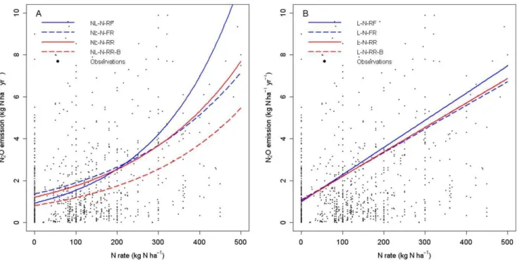
Figure 1. Fitted response curves obtained with the four selected nonlinear models (A) and the four selected linear models (B).Black points correspond to N2O data (96.04% of available observations are displayed; the other data are too extreme for graphical presentation). doi:10.1371/journal.pone.0050950.g001
Figure 2. Fitted response curves for four experiments (exp 1: (A–B), exp 2: (C–D), exp 3: (E–F) and exp 4: (G–H)).For each published-experiment, mean response (solid black line) and experiment-specific response (dotted black line) were calculated with model NL-N-RR (A, C, E, G) and model L-N-RR (B, D, F, H). Black points represent N2O data averaged over replicates.
with eijk,N 0,t2
, a0i,N(m0,s20)and a1i,N m1,s21
Model L-0-F: (6) Yijk~m0zeijk
witheijk,N 0,t2
Model L-N-FF: (7) Yijk~m0zm1Xijzeijk
witheijk,N 0,t2
Model L-0-R: (8) Yijk~a0izeijk
witheijk,N 0,t2anda0i,N m0,s20
Model L-N-RF: (9) Yijk~a0izm1Xijzeijk
witheijk,N 0,t2anda0i,N m0,s20
Model L-N-FR: (10)Yijk~m0za1iXijzeijk
witheijk,N 0,t2anda1i,N m1,s21
Model L-N-RR: (11)Yijk~a0iza1iXijzeijk
with eijk,N 0,t2, a0i,N m0,s20and a1i,N m1,s21
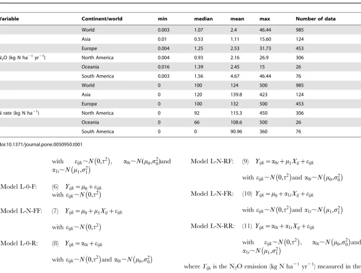
whereYijkis the N2O emission (kg N ha21yr21) measured in the Table 1.Minimal, maximal, median and mean values of nitrous oxide (N2O) and amount of applied N (N rate) for the world and for
North America, South America, Asia, Europe and Oceania.
Variable Continent/world min median mean max Number of data
World 0.003 1.07 2.4 46.44 985
Asia 0.01 0.53 1.11 15.60 124
Europe 0.004 1.25 2.53 31.73 453
N2O (kg N ha21yr21) North America 0.004 0.93 2.16 26.9 306
Oceania 0.016 1.39 2.45 15 26
South America 0.003 1.56 4.67 46.44 76
World 0 100 124 500 985
Asia 0 120 139.8 423 124
Europe 0 100 132 500 453
N rate (kg N ha21) North America 0 92 115.3 450 306
Oceania 0 66 108.6 500 26
South America 0 0 90.96 360 76
doi:10.1371/journal.pone.0050950.t001
Table 2.Characteristics of the 13 statistical models for N2O emission.
Model name Linear
Amount of
N applied Intercept
Effect of the amount of N
applied AIC % AIC BIC % BIC DIC
NL-N-FF No Yes Fixed Fixed 5513.1 23.0 5527.8 22.6 –
NL-0-R No No Random – 5091.9 13.6 5106.5 13.3 –
NL-N-RF No Yes Random Fixed 4553.9 1.6 4573.5 1.5 –
NL-N-FR No Yes Fixed Random 4598.9 2.6 4618.5 2.5 –
NL-N-RR No Yes Random Random 4482.7 0 4507.1 0 –
NL-N-RR-B No Yes Random Random – – – – 4196.71
L-0-F Yes No Fixed – 5653.9 20.5 5663.7 20.1 –
L-N-FF Yes Yes Fixed Fixed 5512.1 17.4 5526.8 17.2 –
L-0-R Yes No Random – 5268.5 12.3 5283.2 12.0 –
L-N-RF Yes Yes Random Fixed 5117.4 9.0 5136.9 8.9 –
L-N-FR Yes Yes Fixed Random 4698.0 0.1 4717.5 0 –
L-N-RR Yes Yes Random Random 4693.2 0 4717.6 0.002 –
L-N-RR-B Yes Yes Random Random – – – – 4421.63
Models were characterized by their response function (linear or exponential), the use of the explanatory variable ‘amount of applied N’, the use of random effects for the intercept and/or the effect of the amount of N applied, values of the Akaı¨ke and Schwartz criteria (AIC and BIC), and of the deviance information criterion (DIC) for Bayesian models. % AIC and % BIC indicate the percentage increase in AIC and BIC with respect to the best linear and nonlinear models.
ithpublished experiment (i= 1 … 203), thejthapplied N dose (j= 1 … Ni), and thek
th
replicate (k= 1 … Kij),Xijis thej
th
applied N dose (kg N ha21) in theithpublished experiment,
m0is the mean
background emission, a0i is the published experiment-specific
background emission (random), m1is the mean applied N effect,
a1iis the published experiment-specific applied N effect (random),
andeijkis the residual error term. The random termsa0i,a1iand
eijk were assumed to be independent and normally distributed.
Models including correlateda0ianda1iwere also fitted to the data
but, as their outputs were very similar to the outputs of the models with independent random parameters, they were not considered further. Note that, in nonlinear models (1–5), the N2O response
does not follow a normal distribution, even if its parameters a0i
and a1ido, due to the use of an exponential function to relate
emissions to model parameters.
In the linear models (6–11), the parameterm1corresponds to the
emission factor EF used by the IPCC. In the nonlinear models based on an exponential function (1–5), N2O emission per unit of
applied N is not constant; instead, it increases as a function of X if
m1 is positive. In the models including one or two random
parameters (2–5 and 8–11), the response of N2O to the amount of
applied N is assumed to follow the same function (linear or exponential) in all experiments, but the parameters of these models (background emission a0i, effect of applied Na1i, or both) were
assumed to vary between experiments. Distributions ofa0ianda1i
describe the between-experiment variability of background emis-sion and N fertilizer effect. An intercept was included in all statistical models to account for background anthropogenic N2O
emission [18]. The values of them0,m1,s0,s1, andtparameters
of models 1–11 were estimated by an approximate maximum likelihood method, with the nlme R statistical package [29].
Two additional models, NL-N-RR-B and L-N-RR-B, were defined. These models were based on the equations of models NL-N-RR and L-NL-N-RR, respectively, but their parameters were estimated by a Bayesian method implemented with a Markov chain Monte Carlo algorithm (MCMC). Normal and independent prior probability distributions were defined for m0 and m1; m0,
m1,N(0,1000). Uniform and independent prior probability
distributions were defined for t, s0, s1; t, s0, s1,U(0,100).
Under these assumptions,m0andm1had a prior mean of zero and
a prior standard deviation of 32, which is quite large given the measured values, which ranged from 0.003 to 46.44 in our dataset. These distributions represent a broad a priori distribution with respect to the data obtained. For example, the 95% credibility interval derived from the prior distributions ranged from26272.3
to 6331.8 N2O kg N ha21yr21for X = 100 kg N ha21. Posterior
distributions of the parameters of models NRR-B and L-N-RR-B were calculated with WinBUGS software [30], with three chains of 100,000 MCMC iterations. Convergence was checked with the Gelman-Rubin method [31].
Model Assessment and Uncertainty Analysis
The Akaike information criterion (AIC) and the Schwartz criterion (BIC) [32,33] were calculated for the first 11 models, and the deviance information criterion (DIC) [34] was calculated for the two Bayesian models. Lower values of AIC, BIC or DIC are considered to indicate better models. Note that the weighting of the experiments according to their lengths did not reduce AIC, BIC or DIC.
We calculated the 95% confidence intervals for each model by a bootstrap method [35,36]; data were sampled, with replacement, 500 times, and each model was fitted to each of the generated samples. For the two Bayesian models, 95% credibility intervals
for the predicted N2O emissions were calculated from the
parameter values generated by the MCMC algorithm.
The predictions generated by the three best non-Bayesian linear models, the three best non-Bayesian exponential models (selected with AIC and BIC criteria) and the two Bayesian models were compared with the N2O emissions calculated by the IPCC-Tier1
method: Y = EF*X, where EF is taken as 0.01 [14]. The range of uncertainty on predicted N2O emissions for the IPCC method was
calculated from the minimum and maximum values of EF (0.003 and 0.03, respectively) reported by the IPCC [14]. The emissions due to applied N calculated with the IPCC method were compared with the predictions of the eight selected models minus the values predicted atX= 0.
This uncertainty range was then compared with each of the confidence intervals for the eight selected models. We also compared the lower limit of the IPCC uncertainty range with the lowest of the eight 2.5 percentiles calculated for the eight selected models, and the upper limit of the IPCC uncertainty range with the highest of the eight 97.5 percentiles of the eight selected models. The most extreme 2.5 and 97.5 percentiles obtained with the eight selected models can be interpreted as best-case and worst-best-case emission scenarios, respectively. They correspond to the lowest and highest limits of the confidence intervals calculated for the eight models.
The code used for statistical analysis is available, on request, from the corresponding author.
Results
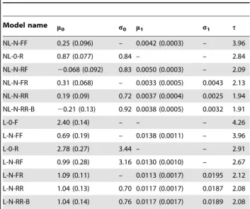
Parameter Values
The estimated value of parameter m0 (mean background
emission) ranged from 20.21 to 0.88 for nonlinear models and
from 0.69 to 2.78 for linear models (Table 3). The between-model variability of the estimated values ofm1(mean applied N effect) was
small: estimated values ranged from 0.0033 to 0.0050 for nonlinear models and from 0.0113 to 0.0138 for linear models. For both linear and nonlinear models, the estimated values ofm1
were lower when the effect of applied N was considered a random
Table 3.Estimated values of the parameters of the 13 models.
Model name m0 s0 m1 s1 t
NL-N-FF 0.25 (0.096) – 0.0042 (0.0003) – 3.96
NL-0-R 0.87 (0.077) 0.84 – – 2.84
NL-N-RF 20.068 (0.092) 0.83 0.0050 (0.0003) – 2.09
NL-N-FR 0.31 (0.068) – 0.0033 (0.0005) 0.0043 2.13
NL-N-RR 0.19 (0.09) 0.72 0.0037 (0.0004) 0.0025 1.94
NL-N-RR-B 20.21 (0.13) 0.92 0.0038 (0.0005) 0.0032 1.91
L-0-F 2.40 (0.14) – – – 4.26
L-N-FF 0.69 (0.19) – 0.0138 (0.0011) – 3.96
L-0-R 2.78 (0.27) 3.44 – – 2.91
L-N-RF 0.99 (0.28) 3.16 0.0130 (0.0010) – 2.67
L-N-FR 1.09 (0.11) – 0.0113 (0.0017) 0.0195 2.12
L-N-RR 1.04 (0.13) 0.70 0.0117 (0.0017) 0.0187 2.08
L-N-RR-B 1.04 (0.14) 0.76 0.0117 (0.0017) 0.0189 2.08
The standard deviations of the estimators ofm0andm1are indicated in brackets.
effect (Table 3). For example, the estimated value ofm1was 0.005
for NL-N-RF, but only 0.0037 for NL-N-RR.
m0 was less accurately estimated than m1; the coefficient of
variation (standard deviation/estimated value) was lower for m1
than for m0. For a given type of function (linear or exponential)
estimates ofs0ands1(between-experiment standard deviation of
background emission and applied N effects, respectively) were similar between models. The estimated values of t (standard
deviation of model residuals) were lower for models with random parameters and for those containing the explanatory variable X.
Model Selection
The lowest AIC and BIC values were obtained for the nonlinear model including two random effects (NL-N-RR) (Table 2). Thus, models based on an exponential function outperformed models based on a linear function. This result was confirmed by the DIC values obtained for the two Bayesian models: DIC was lower with the exponential function.
AIC and BIC values were much higher in models in which applied N (X) was not included as an explanatory variable. The AIC and BIC values of the NL-0-R model were 5091.9 and 5106.5, respectively, whereas the AIC and BIC values of the NL-N-RF model were 4553.9 and 4573.5, respectively (Table 2).
Models including one or two random effects outperformed those including only fixed effects. The best linear model was L-N-RR on the basis of AIC, and L-N-FR, on the basis of BIC. The NL-N-FF (no random effect) model had an AIC of 5513.1 and a BIC of 5527.8, whereas both these values were much lower (AIC = 4482.7 and BIC = 4507.1) for the NL-N-RR (two random parameters) model. Models including one or two random effects had similar AIC and BIC values; the use of one random effect rather than two did not increase AIC and BIC by more than 2.6% and 9% for the nonlinear and linear models, respectively (Table 2).
The AIC and BIC values of models (1), (2), (6), (7) and (8) were more than 10% higher than those for the best nonlinear and linear models, and were therefore not considered further. We therefore considered only models (3), (4), (5), (9), (10) and (11) and the two Bayesian models in our subsequent estimations of N2O emission. Estimation of N2O Emissions with the Selected Models
Figure 1 shows N2O emissions estimated with the eight selected
models. The rate of increase of N2O emissions with the amount of
N applied was greater with the NL-N-RF model (Fig. 1A) than with the other two nonlinear models (NL-N-FR and NL-N-RR). The predicted increase in the amount of N2O emitted per unit
increase in the amount of applied N was thus lower when the effect of applied N was defined as a random effect. Similar results were obtained for linear models, for which the highest rate of increase in N2O emissions with the amount of N applied was obtained for the
L-N-RF model, which had a fixed slope (Fig. 1B). These results are consistent with the estimated parameter values reported in Table 3. The emissions predicted by the Bayesian model NL-N-RR-B were the lowest for all values of applied N (Fig. 1A), due to the low estimated value of the intercept for this model (Table 3). The amounts of emission predicted by the L-N-RR model and its Bayesian counterpart (L-N-RR-B) were very similar and were essentially undistinguishable.
Figure 2 shows the fitted response curves obtained with the best linear and nonlinear models, NL-N-RR and L-N-RR, for four experiments. Considering experiment-specific responses, the non-linear model better fitted the emissions measured at high N doses in experiments 1, 2, and 4, and the emissions measured at low N doses in experiments 3 and 4. Between-experiment variability was high for N2O emissions (Figure 2) and could be accounted for by
the experiment-effects included in the mixed-effect models. The residual standard error was lower with NRR than with L-N-RR (see values oftin Table 3).
Comparison with the Emissions Estimated with the IPCC-Tier 1 Method
We determined the ranges of N2O emissions (Fig. 3) covered by
the eight models considered in Figure 1, either taking into account the uncertainty on the estimated parameter values (dark gray area) or not taking this uncertainty into account (light gray area). The final values predicted by the models were calculated by subtracting the predicted value at X = 0 (background emission) from the value actually predicted for a given amount of applied N. This graphical presentation made it possible to compare our models with the N2O emissions predicted with the IPCC-Tier 1 method. The
estimates of N2O emission obtained with an emission factor of 1%
(as used by the IPCC) were within the range of values covered by the eight selected models (Fig. 3B), but the range of uncertainty for emissions estimated with the IPCC-Tier 1 method was larger than that for the eight selected models. The upper limit of the uncertainty range for the IPCC method was much higher than that defined by the highest value of the eight 97.5 percentiles of the eight selected models, particularly for N applications below 300 kg ha21, as generally practiced in farmers’ fields (Fig. 3). The lower
limits of the uncertainty ranges for the IPCC method and for our models were more similar.
This result was confirmed (Fig. 4) by comparing the estimates of N2O emissions due to applied N obtained with the eight models
with those obtained by the IPCC-Tier 1 method for four different amounts of applied N. These amounts of applied N correspond to the average amounts applied in western, eastern and southern Africa, worldwide, Europe and eastern Asia [10]. The purpose of Figure 4 was to compare model predictions for contrasted applied N doses, not to calculate average emissions at the continental scale. The uncertainty ranges obtained with the IPCC method were indeed larger than those defined by the highest of the 97.5 percentiles and the lowest of the 2.5 percentiles for the eight selected models (Fig. 4). The upper limits of the IPCC uncertainty ranges were systematically higher than the highest 97.5 percentile obtained with our models. We also found that the emissions predicted by the IPCC method were very similar to those obtained with the linear models, but systematically higher than the emissions predicted by the nonlinear models (Fig. 3).
Discussion
Our analysis was carried out with the dataset of Stehfest and Bouwman [10] because this dataset includes a large number of data of N2O emissions in agricultural soils. These data were
collected under various conditions characterized by different measurement methods (e.g. from short to long periods of measurements), different soils, climates, and crops. The variability of these conditions and their effects on N2O emission were taken
into account in our analysis using random parameter models. In these models, the N2O emission was related to applied N using
linear or nonlinear functions including two random parameters (a0i and a1i). The probability distribution of these parameters
Figure 3. Predicted N2O emissions and uncertainty ranges for our eight selected models and the IPCC-Tier 1 method.The light gray
area represents the uncertainty in the model equations and includes the mean values predicted by six models (A) or by eight models (6 non-Bayesian models+2 Bayesian models) (B). The dark gray area represents the uncertainty in model equations and parameter values. The upper and lower limits of the dark gray area indicate the worst-case and best-case scenarios, respectively, defined from six models (A) or from eight models (6 non-Bayesian models+2 Bayesian models) (B). The solid black line and the dotted lines indicate the N2O emissions predicted with an EF of 1% and the uncertainty range of the IPCC-Tier1 method, respectively.
doi:10.1371/journal.pone.0050950.g003
Figure 4. Predicted N2O emissions due to N fertilization and 95% confidence intervals (CI) for each model, and predicted values
and uncertainty ranges for the IPCC-Tier 1 method.The light gray area corresponds to the values covered by the 95% CI of our eight models. The amounts of N applied were A) 16.62 kg N ha21, B) 93.6 kg N ha21, C) 130.74 kg N ha21, D) 149.58 kg N ha21(average amounts of applied N for
western, eastern and southern Africa, worldwide, Europe, and eastern Asia respectively). N2O emissions were estimated by subtracting the value corresponding to the application of no N from the value for each amount of N applied.
Exponential models outperformed linear models for the three statistical criteria considered: AIC, BIC and DIC. However, the differences were small. The AIC of the best linear model was only 4.7% higher than the AIC of the best exponential model. The use of an exponential function rather than a linear model has an important practical consequence: EF is not constant and increases as a function of applied N.
Our results indicate that EF is lower than the estimated value used by the IPCC-Tier 1 (i.e., 1% of applied N) if the amount of N applied is below 160 kg N ha21for the NL-N-RF model, 240 kg N
ha21for the NL-N-FR model and 220 kg N ha21for the
NL-N-RR model. According to Spiertz [27], farmers may apply amounts of nitrogen fertilizer below these thresholds in ecological low-input cropping systems and in some technological high-input systems. Consequently, the use of an exponential model rather than a linear model is likely to decrease estimates of N2O emissions in many
cases. According to Hoben et al. [23], the current IPCC-Tier 1 method could lead to an underestimation of N2O emission if the
true response is exponential. Our results suggest that this is the case only for the application of large amounts of N fertilizer.
McSwiney and Robertson [22] suggested that the use of a nonlinear model instead of a linear model leads to a greater estimated reduction in N2O emission for a moderate reduction in
the amount of applied N, with little or no yield penalty. Our results do not entirely support this statement, because little difference was observed between the two types of models for doses of up to about 200 kg N ha21(Fig. 1). For example, if the amount of applied N is
decreased from 150 kg N to 120 kg N (minus 20%), the resulting reduction of N2O calculated with the NL-N-RR model is 0.22 kg
N ha21yr21, slightly less than that calculated with the current
IPCC emission factor (0.01*30 = 0.3 kg N ha21yr21). With the
same model, the reduction induced by a decrease from 350 kg N ha21to 280 kg N ha21(minus 20%) is much larger, reaching 1 kg
N ha21yr21; this value is higher than the reduction calculated
with the IPCC emission factor (0.01*70 = 0.7 kg N ha21yr21).
The estimated reduction of N2O emission induced by a decrease
in the amount of applied N is greater with the nonlinear model than with the linear model only for high N doses.
According to the AIC and BIC values obtained, models including one or two random effects outperformed models including fixed effects only. Mixed-effect models are commonly used in meta-analysis studies [37] and are recommended for the analysis of repeated measurements on the same individuals [38]. In the dataset of Stehfest and Bouwman [10], N2O emissions were
measured for several amounts of N applied in the same published-experiment. It was therefore appropriate to estimate N2O
emissions with mixed-effect models including one or two random effects in our study (Fig. 2). Models including one or two random effects performed similarly (less than 10% difference in AIC and BIC values), but the estimated effect of the amount of N applied on the amount of N2O emitted tended to be lower when the amount
of N applied was considered as a random effect.
Several models had very similar performances. We therefore used an ensemble approach based on eight models for the estimation of N2O emissions and the definition of uncertainty
ranges. The confidence intervals obtained with the models were used to define lower and upper limits, corresponding to the best-case and worst-best-case scenarios, respectively. These confidence intervals represent the uncertainty in average N2O emissions over
all experiments, but they do not describe the between-experiment variability of N2O emission. The range of uncertainty defined here
is relevant for the Tier 1 method and useful for explorations of the consequences of N applications for average N2O emissions, taking
into account the uncertainty due to model equations and
parameter estimations. The lower limit of our uncertainty range is close to that defined by the IPCC-Tier 1, although our lower limit is slightly higher than that of the IPCC for applications of large amounts of N. Our upper limit is much lower than the upper limit of the IPCC range, particularly for total N applications below 300 kg ha21, as commonly used in agriculture. Thus, the upper
limit of the IPCC range gives an estimated N2O emission of 9 kg
N ha21yr21for a dose of 300 kg N ha21, whereas the upper limit
of our uncertainty range (i.e., the highest upper limit of the confidence intervals of the eight models considered) gave an estimated emission value of only 4.7 kg N ha21yr21. This result is
consistent with the findings of Leip et al. [12], suggesting that the uncertainty on estimates of N2O emissions was overestimated
when derived from experimental data variances, which largely compensate at large scales.
It is useful to compare our uncertainty ranges with other ranges calculated with process-based models [39], top-down methods [40] and hierarchical Bayesian models [16].
Our uncertainty range for the average N dose applied in North America – 0.49–1.88 kg N ha21yr21 – is similar to the 95%
confidence interval proposed by Del Grosso et al. [39] for the United States (133–304 Gg N yr21i.e.0.99–2.27 kg N ha21yr21
with the cropland area of North America reported by Stehfest and Bouwman [10]).
Our uncertainty range for the average N dose applied at the world scale (93.6 kg ha21of applied N, as reported by Stehfest and
Bouwman [10]) (Fig. 4B) – 0.25–1.48 kg N ha21yr21– is lower
and narrower than the interval proposed by Crutzen et al. [40] (2.8–4.68 kg N ha21yr21). However, it is difficult to compare
these intervals, due to the use of a top-down method by Crutzen et al. Furthermore, these authors did not consider direct emission due to N fertilizer only, instead also taking into account indirect emissions from leaching and atmospheric deposition [13].
The 95% confidence interval calculated by Berdanier and Conant [16] with a hierarchical Bayesian linear model is similar to our uncertainty ranges for the four regions of the world presented in Figure 4. The two intervals overlap in all four regions, but our intervals tend to have lower upper and lower limits. For example, Berdanier and Conant [16] reported an interval of 0.05–0.46 for Africa, for a N fertilizer dose of 16.62 kg N ha21[10], whereas our
interval was 0.04–0.26 kg N ha21yr21for the average N fertilizer
dose reported for West, East and Southern Africa by Stehfest and Bouwman [10].
When between-experiment variability was taken into account, the experiment-specific N2O estimated with our models covered a
wider range of values. Thus, for applied N levels of 100 kg N ha21
and with the NL-N-RR model, the 90% percentile for N2O
emission was 1.79 kg N ha21yr21, the 95% percentile was
2.52 kg N ha21yr21 and the 99% percentile was 5.03 kg N
ha21yr21, all these values being higher than the 1 kg N
ha21yr21of the IPCC-Tier 1 method. Thus, N
2O emission has
1% chance to exceed 5 kg N ha21yr21for an N fertilizer dose of
100 kg ha21.
The nonlinear models presented in this paper should be used with caution for estimating average N2O emissions at the country
and continental scales. The average output value of a nonlinear model is not strictly equal to the output value obtained with the average input value. In order to calculate the average N2O
We focused on the Tier 1 approach of the IPCC, but the proposed exponential models could be extended to take several other environmental variables, such as climatic characteristics, soil types and fertilizer type, into account. This possibility has already been explored by Lesschen et al. [13], who took several variables into account (type of fertilizer, crop residues, atmospheric deposition, land use, soil type and precipitation) and by Leip et al. [12], who calculated the stratified emission factor as a function of soil organic carbon content, fertilizer type (mineral
fertilizer or manure) and weather conditions. Such variables could be included in our models, for the estimation of region-specific N2O emissions, taking local characteristics into account.
Author Contributions
Conceived and designed the experiments: AP CL DM. Performed the experiments: AP. Analyzed the data: AP DM. Contributed reagents/ materials/analysis tools: AP DM. Wrote the paper: AP CL DM.
References
1. IPCC (2007) Climate Change 2007: The Physical Science Basis. Contribution of Working Group I to the Fourth Assessment Report of the IPCC. Cambridge: Cambridge University Press.
2. Smith PD, Martino Z, Cai D, Gwary H, Janzen P, et al. (2007) Agriculture. In: Climate Change 2007: Mitigation. Contribution of Working Group III to the Fourth Assessment Report of the Intergovernmental Panel on Climate Change. Cambridge: Cambridge University Press.
3. Galloway JN, Dentener FJ, Capone DG, Boyer EW, Howarth RW, et al. (2004) Nitrogen cycles: past, present and future. Biogeochemistry 70: 153–226. 4. IPCC (2001) Climate Change 2001: The Scientific Basis: Contribution of
Working Group I to the Third Assessment Report of the IPCC. Cambridge: Cambridge University Press. 881p.
5. Mosier A, Kroeze C, Nevison C, Oenema O, Seitzinger S, et al. (1998) Closing the global atmospheric N2O budget: nitrous oxide emissions through the
agricultural nitrogen cycle; OECD/IPCC/IEA Phase II Development of IPCC Guidelines for National Greenhouse Gas Inventories. Nutrient Cycling in Agroecosystems 52: 225–248.
6. Davidson EA (2009) The contribution of manure and fertilizer nitrogen to atmospheric nitrous oxide since 1860. Nature Geoscience 2: 659–662. 7. Snyder CS, Bruulsema TW, Jensen TL, Fixen PE (2009) Review of greenhouse
gas emissions from crop production systems and fertilizer management effects. Agriculture, Ecosystems & Environment 133: 247–266.
8. Rochette P (2008) No-till only increases N2O emissions in poorly-aerated soils.
Soil and Tillage Research 101: 97–100.
9. Rochette P, Tremblay N, Fallon E, Angers DA, Chantigny MH, et al. (2010) N2O emissions from an irrigated and non-irrigated organic soil in eastern
Canada as influenced by N fertilizer addition. 61: 186–196.
10. Stehfest E, Bouwman L (2006) N2O and NO emission from agricultural fields
and soils under natural vegetation: summarizing available measurement data and modeling of global annual emissions. Nutrient Cycling in Agroecosystems 74: 207–228.
11. Rochette P, Worth DE, Lemke RL, McConkey BG, Pennock DJ, et al. (2008) Estimation of N2O emissions from agricultural soils in Canada. I. Development
of a country-specific methodology. Canadian Journal of Soil Science 88: 641– 654.
12. Leip A, Busto M, Winiwarter W (2011) Developing spatially stratified N2O
emission factors for Europe. Environmental Pollution 159: 3223–3232. 13. Lesschen JP, Velthof GL, de Vries W, Kros J (2011) Differentiation of nitrous
oxide emission factors for agricultural soils. Environmental Pollution 159: 3215– 3222.
14. IPCC (2006) Agriculture, Forestry and Other Land Use, Volume 4. In: 2006 IPCC Guidelines for National Greenhouse Gas Inventories. Japan: Institute for Global Environmental Strategies.
15. Lokupitiya E, Paustian K (2006) Agricultural soil greenhouse gas emissions. Journal of Environment Quality 35: 1413–1427.
16. Bernadier AB, Conant RT (2012) Regionally differentiated estimates of croplands N2O emission reduce uncertainty in global calculations. Global
Change Biology 18: 928–935.
17. IPCC (1999) N2O: Direct Emissions from Agricultural Soils. In: Background
Papers: IPCC Expert Meetings on Good Practice Guidance and Uncertainty Management in National Greenhouse Gas Inventories. 361–380.
18. Bouwman AF (1996) Direct emission of nitrous oxide from agricultural soils. Nutrient Cycling in Agroecosystems 46: 53–70.
19. Del Grosso SJ, Ojima DS, Parton WJ, Stehfest E, Heistemann M (2009) Global scale DAYCENT model analysis of greenhouse gas emissions and mitigation strategies for cropped soils. Global and Planetary Change 67: 44–50. 20. Roelandt C, Van Wesemael B, Rounsevell M (2005) Estimating annual N2O
emissions from agricultural soils in temperate climates. Global Change Biology 11: 1701–1711.
21. Freibauer A, Kaltschmitt M (2003) Controls and models for estimating direct nitrous oxide emissions from temperate and sub-boreal agricultural mineral soils in Europe. Biogeochemistry 63: 93–115.
22. McSwiney CP, Robertson GP (2005) Nonlinear response of N2O flux to
incremental fertilizer addition in a continuous maize (Zea maysL.) cropping system. Global Change Biology 11: 1712–1719.
23. Hoben JP, Gehl RJ, Millar N, Grace PR, Robertson GP (2011) Nonlinear nitrous oxide (N2O) response to nitrogen fertilizer in on-farm corn crops of the
US Midwest. Global Change Biology 17: 1140–1152.
24. Millar N, Robertson GP, Grace PR, Gehl RJ, Hoben JP (2010) Nitrogen fertilizer management for nitrous oxide (N2O) mitigation in intensive corn
(maize) production: an emissions reduction protocol for US Midwest agriculture. Mitigation and Adaptation Strategies for Global Change 15: 185–204. 25. Skiba U, Smith KA (2000) The control of nitrous oxide emissions from
agricultural and natural soils. Chemosphere Global Change Science 2: 379–386. 26. Food and Agricultural Organisation (2011) FAO statistic database (FAOSTAT).
Roma. Available: http://faostat.fao.org.
27. Spiertz JHJ (2010) Nitrogen, sustainable agriculture and food security. A review. Agronomy for Sustainable Development 30: 43–55.
28. Tilman D, Cassman KG, Matson PA, Naylor R, Polasky S (2002) Agricultural sustainability and intensive production practices. Nature 418: 671–677. 29. Pinheiro J, Bates D (2000) Mixed-effects Models in S and S-PLUS. 2nded.
NewYork: Springer.
30. Lunn DJ, Thomas A, Best N, Spiegelhalter D (2000) WinBUGS - a Bayesian modelling framework: concepts, structure, and extensibility. Statistics and Computing 10: 325–337.
31. Brooks SP, Gelman A (1998) General methods for monitoring convergence of iterative simulations. Journal of Computational and Graphical Statistics 7: 434– 455.
32. Akaike H (1974) A new look at the statistical model identification. IEEE Transactions on Automatic Control 19: 716–723.
33. Burnham KP, Anderson DR (2002) Model selection and multimodel inference: A practical Information-Theoretic Approach. New York: Springer. 2nd
Ed. 34. Spiegelhalter DJ, Best NG, Carlin BP, van der Linde A (2002) Bayesian
measures of model complexity and fit. Journal of the Royal Statistical Society: Series B 64: 583–639.
35. Efron B, Tibshirani R (1986) Bootstrap methods for standard errors, confidence intervals and other measures of statistical accuracy. Statistical Science 1: 54–75. 36. Efron B, Tibshirani R (1993) An Introduction to the Bootstrap (Chapman &
Hall, London).
37. Philibert A, Loyce C, Makowski D (2012) Assessment of the quality of meta-analysis in agronomy. Agriculture, Ecosystems & Environment 148: 72–82. 38. Davidian M, Giltinan DM (1995) Non linear mixed effect models for repeated
measurement data. Chapman & Hall. 359p.
39. Del Grosso SJ, Ogle SM, Parton WJ, Breidt FJ (2010) Estimating uncertainty in N2O emissions from US cropland soils. Global Biogeochemical Cycles 24: 12pp.
40. Crutzen PJ, Mosier AR, Smith KA, Winiwarter W (2008) N2O release from