Stability Analysis of a Population Dynamics
Model with Allee Effect
Canan Celik
∗Abstract— In this study, we focus on the stability analysis of equilibrium points of population dynamics with delay when the Allee effect occurs at low pop-ulation density is considered. Mainly, mathematical results and numerical simulations illustrate the stabi-lizing effect of the Allee effects on population dynam-ics with delay.
Keywords: Delay difference equations, Allee effect, population dynamics, stability analysis, bifurcation
1
Introduction
Dynamic population models are generally described by the differential and difference equations with or without delay. These models have been considered by many au-thors, for these related results we refer to [1], [4], [6]-[10].
In 1931, Allee [1] demonstrated that a negative density dependence, the so called Allee effect, occurs when popu-lation growth rate is reduced at low popupopu-lation size. The Allee effect refers to a population that has a maximal per capita growth rate at low density. This occurs when the per capita growth rate increases as density increases, and decreases after the density passes a certain value which is often called threshold. This effect can be caused by dif-ficulties in, for example, mate finding, social dysfunction at small population sizes, inbreeding depression, food ex-ploitation, and predator avoidance of defence. The Allee effects have been observed on different organisms, such as vertebrates, invertebrates and plants. (see, for instance, [2], [3]).
The purpose of this paper is to study the following general non-linear delay difference equation with or without the Allee effect
Nt+1=F(λ, Nt, Nt−T), (1) whereλis per capita growth rate which is always positive, Nt represents the population density at timet, T is the time sexual maturity. Here,F has the following form
F(λ;Nt, Nt−T) :=λNtf(Nt−T)
where f(Nt−T) is the function describing interactions (competitions) among the mature individuals. It is gen-erally assumed that f continuously decreases as density
∗TOBB Economics and Technology University, Faculty of Arts
and Sciences, Department of Mathematics, Ankara, Turkey, 06530, E-mail address: [email protected].
increases. Mainly, we work on the stability analysis of this model and compare the stability of this model with or without Allee effects.
Eq. (1) is an appropriate model for single species with-out an Allee effect. Therefore, a natural question arising here is that ”How the stability of equilibrium points are effected when an Allee effect is incorporated in Eq. (1)” . In this work, we answer this question, especially, for the case whenT = 1.
2
Stability analysis of Eq. (1) for
T
= 1
Before we give the main results of this paper, we shall remind the following well-known linearized stability the-orem (see, for instance, [5] and [9]) for the following non-linear delay difference equation
Nt+1=F(Nt, Nt−1). (2)
Theorem A (Linearized Stability). Let N∗
be an equi-librium point of Eq. (2). ThenN∗
is locally stable if and only if
|p|<1−q <2,
where
p:= ∂F ∂Nt
(N∗
, N∗
) and q:= ∂F
∂Nt−1
(N∗
, N∗
).
We now consider the following non-linear difference equa-tion with delay
Nt+1=λNtf(Nt−1) =:F(λ;Nt, Nt−1), λ >0, (3)
where λis per capita growth rate, Nt is the density at time t, and f(Nt−1) is the function describing
interac-tions (competiinterac-tions) among individuals. Firstly, we as-sume thatf satisfies the following conditions:
1◦
f′
(N) < 0 for N ∈ [0,∞); that is, f continuously decreases as density increases.
2◦
f(0) is a positive finite number.
Theorem 1LetN∗
be a (positive) equilibrium point of Eq. (3) with respect to λ. Then N∗
is locally stable if and only if
N∗f ′
(N∗
)
f(N∗) >−1. (4)
Proof. By hypothesis, we have
1 =λf(N∗
). (5)
Let p:= FNt(λ;N
∗
, N∗
). Then, the equality (5) implies that p= 1.Also, observe that
q:=FNt−1(λ;N
∗
, N∗
) =N∗f ′
(N∗
)
f(N∗). (6)
Theorem A says that N∗
is locally stable if and only
|p| < 1−q < 2. Since p = 1, we conclude that N∗
is locally stable if and only if −1 < q <0.However, since f is a decreasing function for allN, we get from (6) that the inequality q < 0 is always valid. So the proof is completed.
Now we find a sufficient condition that increasing λ in Eq. (5) decreases the stability of the corresponding equi-librium points.
Theorem 2Letλ1andλ2be positive numbers such that
λ1< λ2,and letN(1)andN(2)be corresponding positive
equilibrium points of Eq. (3) with respect to λ1and λ2,
respectively. Then the local stability of N(2) is weaker
thanN(1) provided that
N(2) Z
N(1)
[N(logf(N))′
]′dN <0 (7)
holds; that is, increasingλdecreases the local stability of the equilibrium point in Eq. (3) if (7) holds.
Proof. By the definitions ofN(1) andN(2),it is easy to
see that
1 =λ1f(N(1)) and 1 =λ2f(N(2)). (8)
Sinceλ1< λ2,it follows from (8) thatf(N(1))> f(N(2)).
Also, sincef is decreasing function, we haveN(1) < N(2).
Now, for eachi= 1,2, qi:=FNt−1(λi;N
(i), N(i)). Then,
we can easily get that
qi=N(i) f′
(N(i))
f(N(i)) fori= 1,2
holds. So, by Theorem 2.1, each N(i)is locally stable if
and only if
N(i)f
′
(N(i))
f(N(i)) >−1 fori= 1,2. (9)
If the condition (7) holds, then we have
N(1)f
′
(N(1))
f(N(1)) > N (2)f
′
(N(2))
f(N(2)). (10)
Now by considering (9) and (10) we can say that the local stability inN(2)is weaker thanN(1),which completes the
proof.
The following condition is weaker than (7), but it enables us to control easily for increasing λbeing a destabilizing parameter.
Corollary 3Letλ1, λ2, N(1)andN(2)be the same as in
Theorem 2.2. Then the local stability of N(2) is weaker
than that ofN(1) provided that
£
N(logf(N))′¤′
<0 for all N∈[N(1), N(2)]. (11)
RemarkIf there is no time delay in model (3), i.e.,
Nt+1=λNtf(Nt) =:F(λ;Nt), λ >0, (12)
then we have the same result as in theorem 2 where the stability condititon reduces to
N(i)f
′
(N(i))
f(N(i)) >−2 fori= 1,2. (13)
See Example 2 below.
Example 1Consider the difference equation
Nt+1=λNt µ
1−Nt−1
K
, λ >0 andK >0, (14)
with the initial valuesN−1andN0.An obvious drawback
of this specific model is that ifNt−1> K andNt+1<0.
However, if we assume 0< N−1 < K and 0< N0< K,
then, by choosing appropriate λ > 0, we can guarantee that Nt > 0 for any time t. According to this example f(N) = 1−N/K.In this case, we have, for all 0< N < K,
£
N(logf(N))′¤′
=− K
(K−N)2 <0.
So, by Corollary 2, we easily see that if theλ increases, then the local stability in the corresponding equilibrium point of Eq. (14) decreases.
Example 2Consider the difference equation with no de-lay term
Nt+1=λNtexp[r(1−Nt/K)] (15) λ > 0, r > 0 andK > 0,with the initial value N0.
Ac-cording to this model
f(N) = exp[r(1−Nt/K)].
In this case, we have, for allN >0,
£
N(logf(N))′¤′
=−N r K <0.
3
Allee effects on the discrete delay
model (3)
3.1
Allee effect at time
t
−
1
To incorporate an Allee effect into the discrete delay model (3) we first consider the following non-linear dif-ference equation with delay
Nt+1=λ∗Nta(Nt−1)f(Nt−1) =:F(a −)
(λ;Nt, Nt−1),
(16) where λ∗
>0 and the functionf satisfies the conditions 1◦
and 2◦
. As stated in the first chapter, the biological facts lead us to the following assumptions ona:
3◦
ifN = 0,then a(N) = 0; that is, there is no repro-duction without partners,
4◦
a′
(N) >0 for N ∈ (0,∞); that is, Allee effect de-creases as density inde-creases,
5◦
limN→∞a(N) = 1; that is, Allee effect vanishes at
high densities.
By the conditions 1◦ −5◦
, Eq. (16) has at most two positive equilibrium points which satisfy the equation of
1 =λ∗
a(N)f(N) :=h(N).
Assume now that two equilibrium points N∗
1 and N
∗
2
(N∗
1 < N
∗
2) exist so that we haveh(N
∗
1) =h(N
∗
2) = 1.In
this case, by the mean value theorem, there exists a crit-ical point Nc such thath
′
(Nc) = 0 and N
∗
1 < Nc< N
∗
2.
Then we have the following theorem.
Theorem 4 The equilibrium point N∗
1 of Eq. (16) is
unstable. On the other hand,N∗
2 is locally stable if and
only if the inequality
N∗ 2 µ a′ (N∗ 2) a(N∗ 2) +f ′ (N∗ 2)
f(N∗
2)
>−1 (17)
holds.
Proof. Notice that since for eachi= 1,2, N∗
i is positive equilibrium point of Eq. (16), we have
p∗
i :=F
(a−)
Nt (λ
∗
, N∗
i, N
∗
i) =λ
∗
a(N∗
i)f(N
∗
i) = 1
and
q∗
i :=F
(a−)
Nt−1(λ
∗
, N∗
i, N
∗
i) =N
∗ i µ a′ (N∗ i) a(N∗ i) +f ′ (N∗ i) f(N∗
i) 
.
(18) Then, by Theorem A, we get
N∗
i is stable ⇔ |p
∗
i|<1−q
∗
i <2
⇔ −1< q∗
i <0 for i= 1,2.
Since N∗
1 ∈(0, Nc), it is easy to see thatq1∗ >0,which
implies that N∗
1 must be unstable. On the other hand,
forN∗
2 ∈(Nc,+∞) the inequalityq2∗<0 always holds so
that N∗
2 is locally stable if and only if (17) holds.
Now, chooseλ=λ∗
a(N∗
2) and consider the following
Nt+1=λNtf(Nt−1) =:F(λ;Nt, Nt−1) (19)
Then observe that N∗
2 is also positive equilibrium point
of Eq. (19). Furthermore, since a(N∗
2) < 1 and λ =
λ∗
a(N∗
2),we getλ < λ
∗
.
We have the following result.
Theorem 5 The Allee effect increases the stability of the equilibrium point, that is, the local stability of the equilibrium point in Eq. (16) is stronger than that of in Eq. (19).
Proof. By the definition ofa, for eachi= 1,2,we get
N∗
2
µa′
(N∗ 2) a(N∗ 2) ¶ >0, which yields N∗ 2 f′ (N∗ 2)
f(N∗
2)
< N∗
2
µa′
(N∗ 2) a(N∗ 2) +f ′ (N∗ 2)
f(N∗
2)
. (20)
Now considering (20), Theorem 2 and Theorem 3.1 we can say that the stability in Eq. (16) is stronger than the stability in Eq. (19).
Observe that Theorem 5 implies the following result.
Corollary 6There is a locally stable equilibrium point for Eq. (16) such that it is unstable for Eq. (3)
3.2
Allee effect at time
t
In this part we incorporate an Allee effect into the discrete delay model (3) as follows:
Nt+1=λNta(Nt)f(Nt−1) =:F(a
+)
(λ;Nt, Nt−1). (21)
Assume now that N∗
1 and N
∗
2 (N
∗
1 < N
∗
2) are positive
equilibrium points of Eq. (21).
Then we have the following theorem.
Theorem 7 We get thatN∗
1 is an unstable equilibrium
point of Eq. (21). On the other hand,N∗
2 is locally stable
if and only if the inequality
N∗
2
f′
(N∗
2)
f(N∗
2)
>−1. (22)
holds.
Proof. Since, for eachi= 1,2, N∗
i is positive equilibrium point of Eq. (16), we have
p∗
i :=F
(a+)
Nt (λ
∗
, N∗
i, N
∗
i) = 1 +N
and q∗
i :=F
(a−)
Nt−1(λ
∗
, N∗
i, N
∗
i) =N
∗
i f′
(N∗
i) f(N∗
i) .
Then, by Theorem A, we get for eachi= 1,2
N∗
i is stable ⇔ |p
∗
i|<1−q
∗
i <2
⇔ 1 +N∗
i a′(N∗
i)
a(N∗
i) <1−N
∗
i f′(N∗
i)
f(N∗
i) <2.
⇔ N∗
i a′(N∗
i)
a(N∗
i) <−N
∗
i f′(N∗
i)
f(N∗
i) <1
i.e.,
N∗
i µ
a′
(N∗
i) a(N∗
i) +f
′
(N∗
i) f(N∗
i) 
<0<1 +N∗
i f′
(N∗
i) f(N∗
i) .
SinceN∗
1 ∈(0, Nc),it is easy to see that
N∗
1
µa′
(N∗
1)
a(N∗
1)
+f
′
(N∗
1)
f(N∗
1)
>0,
which implies that N∗
1 is an unstable equilibrium point.
Furthermore, since N∗
2 ∈(Nc,+∞),the inequality
N∗
2
µa′
(N∗
2)
a(N∗
2)
+f
′
(N∗
2)
f(N∗
2)
<0
always holds. So N∗
2 is locally stable if and only if (22)
holds.
Let N∗
be a positive equilibrium point of Eq. (3). So, by the choice of λ=λ∗
a(N∗
),N∗
is also an equilibrium point of Eq. (21). In this case, combining Theorem 1 with Theorem 7, we get the following result at once.
Corollary 8 Equilibrium point N∗
is locally stable for Eq. (21) if and only if it is locally stable for Eq. (3).
4
Numerical simulations
In this section, we numerically verify our analytical re-sults (or theorems) obtained in previous sections by using MATLAB programming. In Matlab programs, by taking the initial conditions of the population density as N−1
and N0 in the difference equations we compute Ni’s for the model that we discussed in previous sections. After computingNi’s, mainly we illustrate the graph of the tra-jectory of models in 2D graph in which we can see the stability of equilibrium points. Note that in each graph, we connect the discrete points of population by straight lines.
As we prove analytically in Theorem 2, if we graph the population density functionNtwith respect tot(time) in the model (14) of Example 1, we can easily see in Figure 1- (a)-(b)-(c) that as the parameterλincreases, the local stability of the equilibrium points decreases.
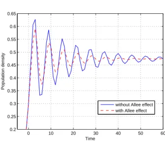
In Figure 2 we graph the 2D trajectory of the population dynamics model (14) respectively with and without Allee
0 10 20 30 40 50 0.2
0.25 0.3
Time
Population density
(a)
0 10 20 30 40 50 0.2
0.3 0.4 0.5
Time
Population density
(b)
0 50 100 0.2
0.25 0.3 0.35 0.4 0.45 0.5 0.55 0.6 0.65 0.7
Time
Population density
(c)
Figure 1: Density-time graphs of the model (14) with K= 1 and the initial conditionsN−1= 0.2 andN0= 0.3.
(a)λ= 1.4. (b)λ= 1.7. (c)λ= 1.95.
0 10 20 30 40 50 60 0.2
0.25 0.3 0.35 0.4 0.45 0.5 0.55 0.6 0.65
Time
Population density
without Allee effect with Allee effect
Figure 2: Density-time graphs of the models Nt+1 =
λNt(1−Nt−1/K) andNt+1=λ∗Nta(Nt−1)(1−Nt−1/K)
with K = 1,λ= 1.9, a(Nt−1) =Nt−1/(α+Nt−1), α=
0.03, λ=λ∗
a(N∗
) and the initial conditionsN−1= 0.2
effect at timet−1, which verifies our Theorem 4. In these figures we take the Allee effect function as a(Nt−1) =
Nt−1/(α+Nt−1), whereαis a positive constant. As we
can see from the graph that population density function obviously verify that when we impose the Allee effect at timet−1 into our model in Example 1, the local stability of the equilibrium point increases and trajectory of the solution approximates to the corresponding equilibrium point much faster.
1.9 2 2.1 2.2 2.3 2.4 2.5 2.6 0
0.5 1 1.5 2 2.5
Growth rate Nt+1
/Nt
Figure 3: Bifurcation diagram of the models in Figure 2 withK= 1, α= 0.06,λ= 1.9 : 0.001 : 2.3,λ=λ∗
a(N∗
) and the initial conditionsN−1= 0.2 andN0= 0.3.
Finally, Figure-3 shows bifurcation diagram of the model in Example 1 as a function of intrinsic growth rateλ with-out the Allee effect (on the left) and with the Allee effect (on the right). In this numeric simulations, N−1 = 0.2
and N0 = 0.3 are taken as the initial conditions as in
the previous calculations. Here we again take the Allee function as a(Nt−1) = Nt−1/(α+Nt−1), where α is a
positive constant. It is obvious from the graph that the comparison of bifurcation diagrams still verifies the sta-bilizing effect of Allee effect. Besides this result, we also observed that the Allee effect diminishes the fluctuations in the chaotic dynamic which is different from the results obtained in the former studies.
5
Conclusions and remarks
Previous studies demonstrate that Allee effects play an important role on the stability analysis of equilibrium points of a population dynamics model (see, for example, [10] and [6]). Generally, an Allee effect has a stabilizing effect on population dynamics. In this paper, we consider a second order discrete models (i.e. with delay), where increasing per capita growth rate decreases the stability of the fixed point. First, we characterized the stability of equilibrium point(s) of this model. Imposing an Allee
effect into the system, the stability of equilibrium points were also studied. Keeping the normalized growth rate the same, we compared the stability of the same equilib-rium point corresponding to the model with and without Allee effect.
Acknowledgement: This study includes some results of ”Allee effects on population dynamics with delay”, (C. C¸ elik, H. Merdan, O. Duman, ¨O. Akın), Chaos, Soli-tons and Fractals.
References
[1] Allee WC. Animal Aggretions: A Study in Gen-eral Sociology, University of Chicago Press, Chicago, 1931.
[2] Beddington JR. ”Age distribution and the stabil-ity of simple discrete time population models”, J. Theor. Biol. V47, pp.65-74,74.
[3] Birkhead TR. ”The effect of habitat and density on breeding success in the common guillemot (uria aalge)”,J. Anim. Ecol.V46, pp.751-64, 77.
[4] Chen J and Blackmore D. ”On the exponentially self-regulating population model”, Chaos, Solitons & Fractals, V14, pp.1433-50, 02.
[5] Cunningham K, Kulenovi´c MRS, Ladas G and Val-icenti SV. ”On the recursive sequences xn+1 =
(α+βxn)/(Bxn+Cxn−1)”, Nonlinear Anal., V47,
pp.4603-14, 01.
[6] Fowler MS and Ruxton GD. ”Population dynamic consequences of Allee effects”,J. Theor. Biol., V215, pp.39-46, 02.
[7] Gao S and Chen L. ”The effect of seasonal harvesting on a single-species discrete population model with stage structure and birth pulses”,Chaos, Solitons & Fractals, V24, pp.1013-23, 05.
[8] Hadjiavgousti D and Ichtiaroglou S. ”Existence of stable localized structures in population dynamics through the Allee effect”, Chaos, Solitons & Frac-tals, V21, pp.119-31, 04.
[9] Kulenovi´c MRS, Ladas G and Prokup NR. ”A ratio-nal difference equation” Comput. Math. Appl. V41, pp.671-8, 01.