ISSN 0101-8205 www.scielo.br/cam
Weak Allee effect in a predator-prey system
involving distributed delays
PAULO C.C. TABARES1∗, JOCIREI D. FERREIRA2∗∗ and V. SREE HARI RAO3∗∗,∗∗∗
1Universidad del Quindío, Facultad de Ciencias Básicas y Tecnologías
Armenia, Quindío – Colombia
2Universidade Federal de Mato Grosso, Instituto de Ciências Exatas e da Terra
Pontal do Araguaia – MT – Brasil
3On leave from Jawaharlal Nehru Technological University
Hyderabad-500 085, India
E-mails: [email protected] / [email protected] / [email protected]
Abstract. In this paper we study the influence ofweak Allee effectin a predator-prey system model. This effect is included in the prey equation and we determine conditions for the occur-rence of Hopf bifurcation. The stability properties of the system and the biological issues of the memory and Allee models on the coexistence of the two species are studied. Finally we present some simulations which allow one to verify the analytical conclusions obtained.
Mathematical subject classification: Primary: 34C25; Secondary: 92B05.
Key words: weak Allee effect, population dynamics, Hopf bifurcation, predator-prey model,
distributed delay.
#CAM-302/10. Received: 01/XII/10. Accepted: 19/IV/11.
∗Research supported by Master program of Biomathematics, UNIQUINDIO, Colombia ∗∗Research supported by FAPEMAT – Fundação de Amparo à Pesquisa do Estado de Mato Grosso, Grant Number 462997/2009.
1 Introduction
It is well known that in nature some species often co-operate amongst them-selves in their search for food or when they try to escape from predators. Allee [15, 16], has studied extensively the aspects of aggregation and associated co-operative and social characteristics among the members of a species. In population biology Allee effect refers to a population that has a maximal per capitagrowth rate at intermediate density. This occurs when the per capita growth rate increases with the increase in the density and decreases when the density passes through a critical value. Clearly this situation is different from the logistic growth in which the per capitagrowth rate is a decreasing func-tion of the density. Even more, when considering coexistence for a single prey species with one or more predator species, then the Allee effect zone is modified, because it depends also on the functional response (see in [6]).
The Allee effect is called weak if there exists no critical density population, below which the per capita rate becomes negative. Taking into account the carrying capacity of the environment with respect to the prey in theper capita growth rate of the population, the weak Allee effect has been modeled in [4] by the following differential equation
˙
N(t)= ε
KN 2(t)
1− N(t) K
(1)
in which N(t) denotes the prey population at time t, 0 < ε < 1 is the per capita growth rate of the population and K > 0 is the carrying capacity of the environment.
In this study we propose and analyze the following system of equations
˙
N(t) = 4ε
K N 2
(t)
1− N(t) K
−αN(t)P(t)
˙
P(t) = −γP(t)+aβP(t)
Z t
−∞
N(τ )exp(−a(t−τ ))dτ (2)
as a model to describe the dynamical behavior of the predator-prey system in-corporating a weak Allee effect in the prey populations N(t)and a distributed delay in the predator populations P(t), at time t. The parameters K, ε, α, γ,
with respect to the prey,ε is the intrinsic growth rate of the prey,α is the rate of predation,γ is the predator mortality in the absence of prey, β is the con-version rate andais the delay parameter. Sinceεis small, we have considered a magnification ofεby denoting it as 4εin the model equations (2) and in the subsequent simulations. This magnification renders clarity to the simulations carried in this paper.
It is well known in biology that group defence helps decrease (or even pre-vent) the predation due to the enrichment in the ability of the prey to defend or escape from the predators. In view of the considerations in Freedman and Wolkowicz [11], the model equations (2) may also be viewed as a predator-prey system with group defence exhibited by the predator-prey.
The models considered in earlier studies ([1, 2, 3, 5, 7, 8, 10, 12, 14]) though similar, but our model differs from those in terms of incorporating weak Allee effect as opposed to a logistic functional response in the prey dynamics. Though our study in this paper allows one to replace the density function ae−at by a more general function G : [0,∞) → [0,∞), that satisfies G(t) ≥ 0 and
R∞
0 G(t)dt =1, we prefer to retain the second equation in the system (2) in its present form, as no new ideas would be introduced by this replacement.
The present paper is organized as follows: In Section 2, we determine the equilibria and present the local stability of the equilibrium points that do not depend on the parameters of the system. The conditions for occurrence of Hopf bifurcation for the parameter dependent equilibrium and the related analysis are discussed in Section 3. The simulation results are carried using Maple 9 and are described in Section 4. A pseudo Maple code that facil-itates the simulations is presented in Section 6. A discussion follows in the final section.
2 Equilibria and the linear analysis
In order to determine the equilibria for the system (2), we rewrite (2) in the following form
˙
N(t) = 4ε
K N 2
(t)
1− N(t) K
−αN(t)P(t)
˙
P(t) = −γP(t)+βP(t)Q(t) ˙
in which
Q(t)=a
Z t
−∞
N(τ )exp(−a(t−τ ))dτ.
The change of variables,
N =K n, P =K p, Q=K q and t = s
ε,
transforms the system (3) into
x′= f(x,K)=
4n2(1−n)−αK ε np,−
γ ε p+
βK
ε pq,
a
ε (n−q)
, (4)
where the prime represents the derivative respect tos,x =(n,p,q) ∈ R3and K ∈(0,∞). It is easy to see that system (4) has the following equilibria
(n1,p1,q1) = (0,0,0) , (n2,p2,q2)=(1,0,1) and
(n3,p3,q3) =
γ βK,
4εγ (βK−γ )
αβ2K3 ,
γ βK
.
The following result provides sufficient conditions for the local stability and equilibria(n1,p1,q1)and(n2,p2,q2).
Proposition 2.1. For the system (4) the equilibrium (n1,p1,q1) is unstable for all K > 0. On the other hand, the equilibrium (n2,p2,q2) is locally asymptotically stable if K < γβ and unstable if K > γβ.
Proof. We establish this result by considering the Jacobian matrix of system (4), which may be written as
J(n,p,q)=
−12εn2
+8εn−αK p
ε
−αK
ε n 0
0 −γ +βK q
ε
βK
ε p
a
ε 0 −
a
ε
. (5)
Similarly the eigenvalues associated with J(n2,p2,q2) are given by −1,
−aε and −γ+βK
ε . Thus (n2,p2,q2) is locally asymptotically stable provided
K < γβ and unstable whenK > γβ.
Remark 2.2. The instability of the origin (n1,p1,q1) may be interpreted as the non vanishing of the species simultaneously in increasing time. On the other hand the instability of the equilibrium (n2,p2,q2) implies that the car-rying capacity of the environmentK and the conversion rateβof the predators do not support the predator population which vanishes in time. This conclu-sion is the same as observed in ([9]). The equilibrium
γ βK,
4εγ (βK−γ ) αβ2K3 ,
γ βK
is biologically meaningful only if
βK −γ >0 or γ
βK <1. (6)
The condition (6) means that the dependence on time of the predator growth rate is positive, at least when Q assumes the value K (see [9]). Moreover, 0 < βγK < 1 implies 0 < γK < β, provided that the mortality rate γ of the predator species with respect to the maximum capacity of prey K, must be less than the conversion rateβ. However, for large enough K, it is always true and necessarily (for small populations of prey), this does not ensure the survival of the predator species.
We shall discuss the stability of this equilibrium in the next section.
3 Stability analysis of the equilibrium(n3,p3,q3)
In this section we study the stability properties of the equilibrium(n3,p3,q3)=
γ βK,
4εγ (βK−γ ) αβ2K3 ,
γ βK
. We study the local codimension one Hopf bifur-cation which occurs in the system (4) and also determine the direction of the bifurcation.
The Jacobian matrix in(n3,p3,q3)is given by
J(n3,p3,q3) =
4γ (βK −2γ )
β2K2 −
αγ
βε 0
0 0 4γ (βK −γ )
αβK2 a
ε 0 −
a
ε
and the characteristic equation associated withJ(n3,p3,q3)is
λ3+ aβ
2K2
+4γ ε (2γ −βK)
β2εK2 λ
2
+4aγ (2γ −βK)
β2εK2 λ+
4aγ2(βK
−γ )
β2ε2K2 =0. (7)
The following proposition is a direct consequence of the Routh-Hurwitz stabil-ity criterion (see [8]).
Proposition 3.1. The critical point(n3,p3,q3)is locally asymptotically stable for the system(4)if the following inequalities are satisfied
βK−γ >0 (8)
2γ −βK >0 (9)
aβ2K2+4γ ε (2γ −βK)
β2εK2 ×
4aγ (2γ −βK)
β2εK2 −
4aγ2(βK−γ )
β2ε2K2 >0. (10)
Remark 3.2. The condition (8) coincide with (6). The same is observed in [8]. From (8) and (9), it follows that
β
2 <
γ
K < β.
Clearly this inequality highlights the contribution of the weak Allee effect, i.e. the refinement in the relationship betweenβ,γ andK.
A rearrangement of terms in (10) yields
a> γ 16βγ εK −16γ
2ε
−4β2εK2+β3K3−β2γK2
β2K2(2γ −βK) . (11)
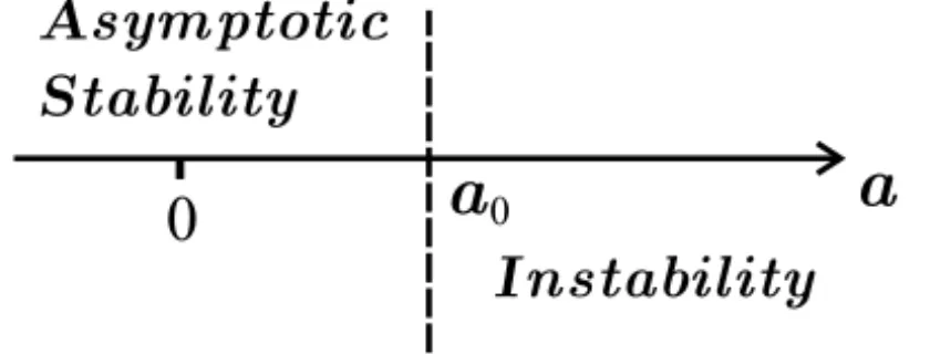
and this inequality is trivially satisfied if the right hand side of (11) is either zero or negative, in which case the equilibrium (n3,p3,q3)is locally asymp-totically stable for alla >0. The case of interest for us would be when
a0= γ 16βγ εK −16γ 2ε
−4β2εK2
+β3K3
−β2γK2
Figure 1 – Critical value of the bifurcation parametera.
In this case, (n3,p3,q3) loses its stability at a = a0 (see Fig. 1). We study the local codimension one Hopf bifurcation which occurs in the system (4) for the state variables(n,p,q)∈R3and the parametera
∈R+.
To simplify the calculations we introduce the notationb = 1
βK and rewrite conditions (8)-(10) respectively as
1
2 < γb<1 (13)
16εγ2b3+4εb−16εγb2−1+γb<0 (14) a0= γ
1−2γb 16εγ 2b3
+4εb−16εγb2−1+γb
. (15)
Ata =a0the eigenvalues of system (4) are given by
λ0(a0)=
γ (γb−1)
ε (2γb−1) <0, λ1,2(a0)= ±iω (16)
in which
ω= 2γ ε
q
εb −16εγ2b3−4εb+16εγb2+1−γb
. (17)
We have the following result
Theorem 3.3. With the notation and conditions(13)-(17)the real part of the eigenvalueλ1(a)that isRe(λ(a))satisfies the conditions that
d
dλ Re λ1(a0)
Proof. Note thatλ1(a0)=iωand define the function F(λ,a) = λ3+a−4εγb+8εγ
2b2
ε λ
2
+4aγb(2γb−1)
ε λ
+ 4aγ
2b(1
−γb)
ε2 (18)
obtained from the right hand side of (7) in whichb= 1
βK.
Since F(λ1(a0) ,a0)= F(iω,a0) =0 andiωis a simple root of F(λ,a0); by the implicit function theorem exist a unique oneλ=λ(a)in a neighborhood ofa0such that
λ′1(a0)= −F ′
a(iω,a0)
F′
λ(iω,a0) ,
where
Fa′(λ,a)= λ
2
ε +
4γb(2γb−1)
ε λ+
4γ2b(1−γb) ε2 and
Fλ′(λ,a)=3λ2+ 2 a−4εγb+8εγ
2b2
ε λ+
4aγb(2γb−1)
ε .
Thus
Fa′(iω,a0)=(2γb−1) −ω2ε−4iωεγb+8iωεγ2b2+4γ2b−4γ3b2
and
Fλ′(iω,a0) = ε(−3ω2ε+6ω2εγb−2iωγ +2iωγ2b−192εγ4b4
+128εγ5b5−16εγ2b2+96εγ3b3+4γ2b
−12γ3b2+8γ4b3).
Since
d da
Re(λ1(a0))
=Re
d
da(λ1(a0))
,
substituting
ω2= 4γ
2b
ε −16εγ
2b3
in Re
d
da(λ1(a0))
we have
Re
d
da(λ1(a0))
=−2b(2γb−1)
2 16εγ2b3
+4εb−16εγb2−1+γb
G(ε,∙) , (19)
where
G(ε,∙) = 256ε2γ4b6−512ε2γ3b5+16εγ3b4+384ε2γ2b4−32εγ2b3
−γ2b2−128ε2γb3+20εγb2+2γb+16ε2b2−4εb−1.
From (14) the numerator in the right hand side of (19) is positive. To complete the proof we need to show thatG(ε,∙)6= 0. To this end, consider the equation G(ǫ)=0, and observe that
ε1=
√
5−1(γb−1)
8b(2γb−1)2 <0 and ε2=
√
5+1(1−γb)
8b(2γb−1)2 >0,
are its roots. SinceG′′(ε,∙) =32b2(2γb−1)4 > 0,G has a minimum in the interval(ε1, ε2). Rewriting (14) as
0< ε < 1−γb
4b(2γb−1)2,
we have
0< ε < 1−γb
4b(2γb−1)2 <
√
5+1(1−γb)
8b(2γb−1)2 =ε2.
So, G(ε,∙) < 0 which implies Re
d
da[λ1(a0)]
< 0, and this proves the
Theorem.
Now we introduce the new bifurcation parameterμby
a(μ)= a0
1+a0μ (20)
bifurcation point. Further,
Re
d
dμ[λ1(a(μ))]
μ=0
= 2γ
2b 16εγ2b3
−16εγb2
+γb+4εb−13 G(ε,∙) >0.
3.1 Projection to the center manifold
At beginning of this section we show that the eigenvalues curve of system (4) satisfies the transversality conditions of the Hopf’s Theorem. In the following, we will restrict system (4) to the center manifold, that is, we will project the vector field associated to system (4) to the center manifold. So, the ODE system given by (4) will behave as a system on plane.
To reach this purpose, we consider the change of variables b = β1K to convert the equilibrium(n3,p3,q3)to the form
γb,4εγbα(1K−γb), γb
. Further-more, we move this equilibrium to origin introducing the variables
x =n−γb, y = p−4εγb(1−γb)
αK , z =q−γb. (21)
Thus, with the new variables we carried out system (4) to the equivalent system
˙
x = 4(x +γb)2(1−(x +γb))− αK
ε (x+γb)
y+4εγb(1−γb)
αK
˙
y = −γ
ε
y+ 4εγb(1−γb)
αK
+ 1
εb
y+4εγb(1−γb)
αK
(z+γb)
˙
z = a0
ε (1+a0μ)(x +γb−(z+γb))
Atμ=0 (i.e. ata=a0) we have
˙
x = −4x3−12γbx2+4x2−8γ2b2x +4γbx− αK
ε x y− αKγb
ε y
˙
y = 4γ
αKz− 4γ2b
αK z+
1
εbyz
˙
z = ω
2
The eigenvectors of the above system associated with the eigenvalues
λ0(a0)=
γ (γb−1)
ε (2γb−1) andλ1,2(a0)= ±iωare
s0=
4γ2b2(2γb−1) ω2
ε αK
−1 4(2γb−1)
and s1,2=
1 0 1 ±i
4γb(2γb−1) ω
4γ (γb−1) αωK 0 respectively.
We take s0 and the real and imaginary parts of s1,2 as a new basis for R3. So, with the change of coordinate
x y z =A
x1 x2 x3 (22) where A=
1 4γb(2γb−1)
ω
4γ2b2(2γb
−1) ω2 0 4γ (γb−1)
ωαK
−ε αK
1 0 −1
4(2γb−1)
we transform system (22) to an equivalent system
˙
x1 = ωx2+U1,2(x)+U1,3(x)
˙
x2 = −ωx1+U2,2(x)+U2,3(x) (23)
˙
x3 = γ (γb−1)
ε (2γb−1)x1+U3,2(x)+U3,3(x) ,
forx=(x1,x2,x3)and
U1,2(x) = − 4ω2
D (γb−1) (3γb−1)x 2 1
−16γ
2b
εD (γb−1) (2γb−1) 24εγ 2
+4εb−1x22+
γ2b
4ω2ε2D 16εγ 3
b3+4γ3b3−4γ2b
−7ω2εγb−4ω2ε2b+8ω2ε+3εDx32
− ω
εγb D(γb−1) 48εγ 2b3
−40εγb2+3γb
+8εb−2x1x2+4γ 2b
εD 8εγ 2b3
+3γ2b2−4εγb2
−5γb+2x1x3− 4γb
ωε2D(γb−1) 4εγ 3
b2+γ3b
−4ω2ε2γb−γ2+ε2ω2x2x3
U1,3(x) = − 4ω2
D (γb−1)x 3 1−
256γ3b3
ωD (γb−1) (2γb−1) 3x3
2
−256γ
6b6
ω4D (γb−1) (2γb−1) 3
x33
−48ωγb
D (γb−1) (2γb−1)x 2 1x2
−48γ
2b2
D (γb−1) (2γb−1)x 2 1x3
−192γ
2b2
D (γb−1) (2γb−1) 2x1x2
2
−768γ
4b4
ω2D (γb−1) (2γb−1) 3
x22x3
−192γ
4b4
ω2D (γb−1) (2γb−1) 2x1x2
3
−768γ
5b5
ω3D (γb−1) (2γb−1) 3x2x2
3
−384γ
3b3
ωD (γb−1) (2γb−1)x1x2x3
U2,2(x) = 4ω3ε
+16ωγb
D (2γb−1)
2 24εγ2b3
−20εγb2+γb+4εb−1
x22
−16 γ
ωε2D(2γb−1)(28γ 4b3
−60γ3b2−16εγ2b2
+16ω2ε2γb2−16ε2γb2D+32γ2b−4ω2ε2b
+3εD−ω2ε)x32− 1
2ε2b D(16εγ 3b3
+8ω2ε2γb2+4γ3b2
+48ε2γb2D−4γ2b−3ω2εγb−4ω2ε2b−16ε2b D
+4ω2ε+εD)x1x2+ ω
8εγb D(64εγ 3
b3+4γ3b2−16εγ2b2
−32ω2ε2γb2−4γ2b+8ω2ε2b+3ω2ε)x1x3
− 1
8ε2b D(2γb−1)(16γ 4b3
−36γ3b2−16εγ2b2−32ε2γb2D
+8ω2ε2γb2+20γ2b+4ω2εγb+8ε2b D+2εD−5ω2ε)x2x3,
U2,3(x) = 4ω3ε
γD (2γb−1)x 3 1+
256εγ2b3
D (2γb−1) 4x3
2
+ 256εγ
5b6
ω3D (2γb−1) 4x3
3+ 48ω2b
D (2γb−1) 2x2
1x2
+ 48ωεγb
2
D (2γb−1) 2
x12x3
+ 192ωεγb
2
D (2γb−1) 3x1x2
2+
768εγ3b4
ωD (2γb−1) 4x2
2x3
+ 192εγ
3b4
ωD (2γb−1) 3x1x2
3+
768εγ4b5
ω2D (2γb−1) 4x2x2
3
+ 384εγ
2b3
D (2γb−1)
3x1x2x3
U3,2(x) = − 16ω2
D (γb−1) (2γb−1) (3γb−1)x 2 1
− 64γ
2b
εD (γb−1) (2γb−1) 2
+γb+4εb−1)x22+
γ2b
ω2ε2D(2γb−1) (16εγ 3
b3+4γ3b2
−4γ2b−7ω2εγb−4ω2ε2b+8ω2ε+3εD)x32
− 4ω
εγb D(γb−1) (2γb−1) (32εγ 3
b3−16εγ2b2+4γ2b
−3ω2ε)x1x2+ 2
εD(2γb−1) (32εγ 3
b3+24γ4b3−16εγ2b2
−44γ3b2+20γ2b−ω2ε)x1x3− 16γb
ωε2D(2γb−1) (4εγ 3
b2
+γ3b−4ω2ε2γb−γ2+ω2ε2)x2x3
U3,3(x) = − 16ω2
D (γb−1) (2γb−1)x 3 1
−1024γ
3b3
ωD (γb−1) (2γb−1) 4
x23
−1024γ
6b6
ω4D (γb−1) (2γb−1) 4x3
3
−192Dωγb(γb−1) (2γb−1)2x12x2
−192γ
2b2
D (γb−1) (2γb−1) 2x2
1x3
−768γ
2b2
D (γb−1) (2γb−1) 3x1x2
2
−3072γ
4b4
ωD (γb−1) (2γb−1) 4x2
2x3
−768γ
4b4
ω2D (γb−1) (2γb−1) 3x1x2
3
−3072γ
5b5
ω3D (γb−1) (2γb−1) 4
x2x23
−1536γ
3b3
ωD (γb−1) (2γb−1)
with
D = ω2 −16εγ2b3+16εγb2+γb−4εb−1
+16γ2b2(γb−1) (2γb−1)2= 4γ
2b
ε ×G(ε,∙) .
Now we project the system (23) to the center manifoldMwhich is character-ized by the fact that it is tangent to thex1x2plane at the origin (the eigenspace corresponding toλ1,2 = ±iω) and is locally invariant with respect to the flow of system (23). Note that this center manifold can be parameterized by the variablesx1 andx2 in the form x3 = h(x1,x2) whereh : R2 → Radmits a Taylor expansion of the form
h(x1,x2)= 1
2 h11x 2
1 +2h12x1x2+h22x 2 2
+O
q
x2 1+x22
3!
,
and, theCenter Manifold Theoremimplies thathmust satisfy
0=h(0,0)=h′x
1(0,0)=h ′
x2(0,0) ,
where h∈Ck, k
∈N with k >3.
If (x1(s) ,x2(s) ,x3(s)) is a solution of system (23) near the origin with initial conditions starting on M then the flow of system (23) remains locally onMfor all time, that isx3(s)≡h(x1(s) ,x2(s)). Consequently
˙
x3(s)−h′x1(x1(s) ,x2(s))x1˙ (s)−h′x2(x1(s) ,x2(s))x2˙ (s)≡0.
Using system (23) the above identity turns out to be
γ (γb−1)
ε (2γb−1)x3+U3,2(x1,x2,x3)+U3,3(x1,x2,x3)−h ′
x1(x1,x2)
− h11x1+h12x2+O
q
x21+x22
2!!
ωx2+U1,2(x1,x2,x3)
+ U1,3(x1,x2,x3)
− h12x1+h22x2+O
q
x12+x22
2!!
×
−ωx1+U2,2(x1,x2,x3)+U2,3(x1,x2,x3)
since
x3=h(x1,x2)= 1
2 h11x 2
1+2h12x1x2+h22x 2 2
+O
q
x12+x22
3!
.
Omitting the terms of third and higher order we obtain
γ (γb−1)
2ε (2γb−1) h11x
2
1+2h12x1x2+h22x 2 2
−ωh11x1x2−ωh12x22+ωh12x12+ωh22x1x2≡0.
A rearrangement of terms yields
γ (γb−1)
2ε (2γb−1)h11−
16ω2
D (γb−1) (2γb−1) (3γb−1)+ωh12
x12
+
γ (γb−1)
2ε (2γb−1)h22−
64γ2b
εD (γb−1) (2γb−1) 2
4εγb2(2γb−1)
− ω
2ε 4γ2b
−ωh12
x22+
γ (γb−1) ε (2γb−1)h12−
16ωγb
εD (γb−1) (2γb−1)
×
γb+8εγb2(2γb−1)− ω
2ε 2γ2b
−ωh11+ωh22
x1x2≡0.
Equating the coefficient to zero and solving the resulting system we have
h11 =
32ω2εγb(γb
−1)(2γb−1)2
D×F 8εb(2γb−1) 2
(4γb−1)
+3γ2b2−3γb+1 h12 = −16(γb−1)(2γb−1)
D×F ε 8γ 2b2
(γb−1)(2γb−1)2(4γb−1) −D(3γb−1)−γ2b(γb−1)(6γ2b2−9γb+2)
h22 = 64γb(γb−1)(2γb−1) 3
D×F ε D+8γ 2b2
(2γb−1)(3γ2b2
−3γb+1)+2γ2b(4γb−3)(γb−1),
where
Thus,
h(x1,x2) = 8(γb−1) (2γb−1)
D×F 2Tω 2
εγb(2γb−1)x12
−Rx1x2+4γb(2γb−1)2Sx22
,
where
T = 8εb(2γb−1)2(4γb−1)+3γ2b2−3γb+1
R = ε(8γ2b2(γb−1) (2γb−1)2(4γb−1)−D(3γb−1)) −γ2b(γb−1)× 6γ2b2−9γb+2
S = ε D+8γ2b2(2γb−1) 3γ2b2−3γb+1
+2γ2b(4γb−3) (γb−1) .
Finally, to get to the restriction of system (23) to the μ = 0 section of the center manifoldM, we consider the new change of coordinates
y1=x1, y2=x2, y3=x3−h(x1,x2) .
In this new coordinate system, the equation of theμ =0 section is y3 =0 , that is theμ=0 section is the y1,y2plane. By this coordinate transformation, system (23) becomes
˙
y1 = ωy2+U1,2(y1,y2,y3+h(y1,y2))+U1,3(y1,y2,y3+h(y1,y2))
˙
y2 = −ωy1+U2,2(y1,y2,y3+h(y1,y2))+U2,3(y1,y2,y3+h(y1,y2))
˙
y3 = γ (γb−1)
ε (2γb−1)y3+U3,2(y1,y2,y3+h(y1,y2)) +U3,3(y1,y2,y3+h(y1,y2)) .
Restricted to the center manifoldMwe can writey3=0 everywhere and taking into that y3˙ = 0. Hence, the system (23) restricted to the center manifold is given by
˙
y1 = ωy2−4ω 2
D (γb−1) (3γb−1)y 2 1−
16γ2b
εD (γb−1) (2γb−1)
× 24εγ2b3−20εγb2+γb+4εb−1y22−4ωγ
εD (γb−1) 48εγ 2
−40εγb2+3γb+8εb−2y1y2+4γ 2b
εD 8εγ 2
b3+3γ2b2−4εγb2
−5γb+2
h(y1,y2)y1− 4γb
ωε2D(γb−1) 4εγ 3b2
+γ3b−4ω2ε2γb
−γ2+ε2ω2h(y1,y2)y2−4ω 2
D (γb−1)y 3 1−
256γ3b3
ωD (γb−1)
× (2γb−1)3y23−48ωγb
D (γb−1) (2γb−1)y 2 1y2−
192γ2b2 D
× (γb−1) (2γb−1)2y1y22+O
q
y12+y22
4!
˙
y2 = −ωy1+4ω 3ε
D (2γb−1) (3γb−1)y 2 1+
16ωγb
D (2γb−1) 2
× 24εγ2b3−20εγb2+γb+4εb−1y22+ 1
εb D
×
4ω2εb(2γb−1) 48εγ2b3−40εγb2+γb+8εb−1
(24)
− 4γ
2b(γb
−1)2 ε
y1y2+ ω 4γb D
ω2
−16εγb2+4εb+ 3 2
+ 2γ
2b 16εγb2
+γb−4εb−1
ε
h(y1,y2)y1
+ γ
2
ε2D(2γb−1) 64ε
3b3(2γb
−1)4(4γb−1)
+ (γb−1)2h(y1,y2)y2+4ω 3ε
γD (2γb−1)y 3 1+
256εγ2b3 D
× (2γb−1)4y23+48ω 2b
D (2γb−1) 2y2
1y2
+ 192ωεγb
2
D (2γb−1) 3y1y2
2+O
q
y2 1+y
2 2
4!
.
The calculations may be summarized in the next proposition, which provides the direction of the Hopf bifurcation.
(4). The first Lyapunov coefficient associated with the equilibrium(n3,p3,q3)
is given by
G4 = 1
ωε2γD2F −1048576ωε 6
γ6b8(2γb−1)11(3γb−1)2 −32768ε5γ6b7(γb−1)×(2γb−1)9× 12γ2b2+232ωγ2b2
−7γb−156ωγb+26ω+1−4096ε4γ6b6(γb−1) (2γb−1)7 ×(516ωγ3b3+44γ3b3−68γ2b2−862ωγ2b2+418ωγb
+27γb−62ω−3)−512ε3γ6b5(γb−1) (2γb−1)5 × 720ωγ4b4−24γ4b4−1804ωγ3b3+62γ3b3−59γ2b2
+1632ωγ2b2−632ωγb+25γb+88ω−4
−128ε2γ6b4(γb−1)2(2γb−1)4× 260ωγ3b3−22γ3b3
−466ωγ2b2+43γ2b2+262ωγb−25γb−48ω+4
−32γ6b3(γb−1)4(2γb−1)2(44ωγ2b2+6γ2b2 (25)
−38ωγb−7γb+4ω+2)+16ωγ6b2(γb−1)4 × 28γ3b3−47γ2b2+25γb−4.
Proof. Consider the two dimensional ODE system
˙
x = −ωy+ f2(x,y)+ f3(x,y) ˙
y = ωx+g2(x,y)+g3(x,y) , (26)
where
f2(x,y) = a1x2+a2x y+a3y2,
f3(x,y) = b1x3+b2x2y+b3x y2+b4y4,
g2(x,y) = c1x2+c2x y+c3y2
In accordance with Bautin’s Lemma (see [8]) the first Poincaré-Lyapunov coef-ficient for system (26) is given by
G4= 1
4 3b1+b3+d2+3d4
+ 41 ω
× a1a2+a2a3−c1c2−c2c3+2(a3c3−a1c1).
(27)
Comparing (26) with (24) and using (27), we obtainG4as given by (25).
With the results obtained in this section we can enunciate the following Theorem.
Theorem 3.5. If (12) holds and G4 < 0 (respectively G4 > 0), then there exists aδ > 0such that for each a ∈ a0−δ,a0(respectively a ∈ a0,a0+
δ), the system (4) (or equivalently system (3)) has a unique orbitally asymp-totically stable (respectively unstable) periodic orbit around the equilibrium
(n3,p3,q3).
4 Simulation results
In this section we present some simulations carried in Maple 9 to verify the veracity of the analytical results obtained for system (4).
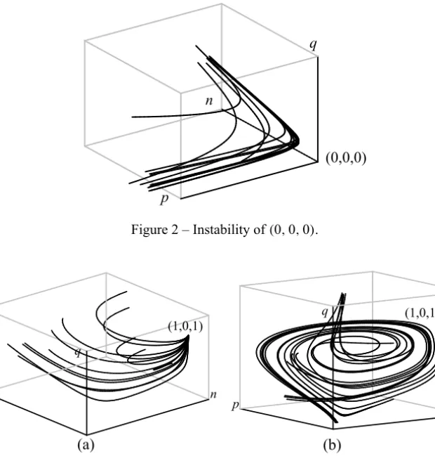
The equilibrium point (0,0,0) is always unstable; to illustrate this case we made the phase portrait in the case by choosingε = 0.5, K = 1.4, α = 0.5,
γ =0.7,β =0.8 ya =0.25 (see Fig. 2).
The equilibrium point (1,0,1) is stable if βK −γ < 0 and unstable if
βK −γ > 0. So, to see the stability of this equilibrium we take ε = 0.5, K = 1.4, α = 0.5, γ = 0.7, β = 0.3 and a = 0.25 (see Fig. 3-(a)); on the other hand, the instability is obtained whenε = 0.5, K = 1.4 , α = 0.5,
γ =0.7,β =0.8 anda =0.25 (see Fig. 3-(b)).
Finally, we illustrate the stability properties of the equilibrium (n3,p3,q3). If we consider the following values of the parameters ε = 0.2, K = 1.4,
α = 0.5, γ = 0.7, β = 0.8 and a = 0.985, the equilibrium (n3,p3,q3)
is asymptotically stable (see Fig. 4-(a)). Note that these values yield
(0,0,0) q
n
p
Figure 2 – Instability of(0,0,0).
(a) q
n
(1,0,1)
p
q
p
(1,0,1)
(b)
n
Figure 3 – Equilibrium(1,0,1): (a) Stable persistence. (b) Unstable persistence.
( n3 , p3 , q3 ) q
.
p
(a)
n n
( n3 , p3 , q3 )
p
.
q(b)
respectively. Furthermore, decreasing the value of a up to a0 we see in Figure 4-(b) that the equilibrium(n3,p3,q3)is aweak stable focus.
The parameters given in the above paragraph we obtain Figures 5 (a) and (b) illustrating the occurrence of a periodic orbit around the equilibrium
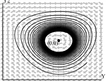
(n3,p3,q3) ata = 0.825 and a = 0.414628 respectively. Note that in this case we haveG4 ≈ −2.595557406 which shows numerically that the periodic orbit generated by the Hopf bifurcation is supercritical anda0 = 0.925 is the bifurcation point. Finally, in Figure 6 we give a phase portrait for system (24), the restriction of system (4) to the center manifold.
( n3 , p3 , q3 )
n
(a)
p
.
q.
( n3 , p3 , q3 )(b)
p
n q
Figure 5 – (a) Periodic orbit ata =0.825. (b) Periodic orbit ata=0.414628.
.
Y2
Y1 (0,0)
5 Maple Code
In this section we include the main Maple code used to simulate Figure 2. The same code is appropriately modified for simulating other figures
> restart:
1
> with(plots):with(DEtools):with(plottools):with(RandomTools):
2
> unprotect(gamma):epsilon:=0.5:K:=1.4:alpha:=0.5:gamma:=0.7:
3
beta:=0.8:a:=0.25:
4
> sist:={diff(x(t),t)=4*x(t)ˆ2*(1-x(t))-alpha*K/epsilon
5
*x(t)*y(t),diff(y(t),t)=-gamma/epsilon*y(t)+1/(epsilon*b)
6
*y(t)*z(t),diff(z(t),t)=a/epsilon*(x(t)-z(t))}:
7
> amin:=0.05:amax:=0.4:
8
> cond:=[[x(0)=Generate(float(range=amin..amax,digits=3)),
9
y(0)=Generate(float(range=amin..amax,digits=3)),
10
z(0)=Generate(float(range=amin..amax,digits=3))]]:
11
> for i from 1 by 1 to 12 do
12
cond:=[op(cond),[x(0)=Generate(float(range=amin..amax,
13
digits=3)),y(0)=Generate(float(range=amin..amax,
14
digits=3)),z(0)=Generate(float(range=amin..amax,
15
digits=3))]]:end do:
16
> xmax:=0.6:ymax:=0.6:zmax:=0.6:
17
> opc:=x=-0.1..xmax+0.07,y=-0.1..ymax+0.07,z=0..zmax+0.07,
18
stepsize=.05,axes=box,linecolor=black,color=grey:
19
> tiempo:=t=-15..15:x1:=0:y1:=0:z1:=0:
20
> espfase:=DEplot3d(sist,{x(t),y(t),z(t)},tiempo,cond,opc,
21
thickness=2,labels=[n,p,q],orientation=[145,55]):
22
> display(espfase,tickmarks=[2,2,2],axes=boxed);
23
Discussion
Stability analysis of the equilibrium states is carried out. Conditions are derived for the occurrence of Hopf bifurcation of the equilibria of this model.
Farkas [8] has considered a predator-prey system similar to that of the pres-ent model with logistic type functional response and with weak Allee effect. The functional response considered in our model is different from that in [8]. Theorem 3.5 is an analogue of Theorem 7.3.1 (see [8]). It is observed that though the weak Allee effect drives the system to instability, the parameters associated with the memory will play a neutralizing role which is evident from the presence of periodic orbits.
Acknowledgments. The authors express their gratitude to late professor Miklós Farkas for the stimulating discussions. The authors wish to thank the anonymous reviewers for their constructive suggestions, which have led to the improvement of our earlier presentation.
REFERENCES
[1] A. Farkas, M. Farkas and L. Kaitar, On Hopf bifurcation in a predator-prey model. Diferential Equations: qualitative theory, pp. 283-290, Amsterdam, North-Holland (1987).
[2] A. Farkas, M. Farkas and G. Szabo, Multiparameter bifurcation diagrams in predator-prey models with time lag. Journal of Mathematical Biology,26(1988), 93–106, Springer-Verlag.
[3] A. Bocsó and M. Farkas, Political and economic rationality leads to velcro bifurcation. Applied Mathematics and Computation,140(2003), 381–389.
[4] D. Boukal and L. Berec, Single-species models of the Allee effect: Extinction boundaries, sex ratios and mate enconunters. Journal of Theoretical Biology, 218(2002), 375–394.
[5] J.M. Cushing, Two species competition in a periodic environment. Journal Mathematical Biology,10(1980), 385–400.
[6] K. Kiss and J. Tóth,n-dimensional ratio-dependent predator-prey systems with memory. Differential Equations and Dynamical Systems, 17(1-2) (2009), 1111– 1141.
[8] M. Farkas,Periodic Motions. Springer-Verlag, New York (1994).
[9] M. Farkas,Dynamical Models in Biology. Academic Press, New York (2001).
[10] N. MacDonald, Time delay in a prey-predatormodels. II. Bifurcation theory. Mathematical Bioscience,33(1977), 227–234.
[11] H.I. Freedman and G.S.K. Wolkowicz, Predator-Prey Systems with Group De-fence: The Paradox of Enrichment Revisited. Bulletin of Mathematical Biology, 48(516) (1986), 493–508. Printed in Great Britain.
[12] N. MacDonald,Time lags in biological models. Lecture Notes in Biomathematics 27, Springer-Verlag, Berlin (1978).
[13] S. Wiggins, Introduction to Applied Nonlinear Dynamical Systems and Chaos. Springer-Verlag, Heidelberg (1990).
[14] V. Volterra,Lecons sur la théorie mathématique de la lutte pour la vie. Gauthier-Villars, Paris (1931).
[15] W.C. Allee,Animal aggregations. Quart. Rev. Biol.,2(1931), 367–398.