www.atmos-meas-tech.net/3/545/2010/ doi:10.5194/amt-3-545-2010
© Author(s) 2010. CC Attribution 3.0 License.
Measurement
Techniques
Measurement of Ozone Production Sensor
M. Cazorla and W. H. Brune
Department of Meteorology, Pennsylvania State University, PA 16802, USA
Received: 1 December 2009 – Published in Atmos. Meas. Tech. Discuss.: 22 December 2009 Revised: 18 April 2010 – Accepted: 20 April 2010 – Published: 3 May 2010
Abstract. A new ambient air monitor, the Measurement of Ozone Production Sensor (MOPS), measures directly the rate of ozone production in the atmosphere. The sensor con-sists of two 11.3 L environmental chambers made of UV-transmitting Teflon film, a unit to convert NO2to O3, and a modified ozone monitor. In the sample chamber, flowing am-bient air is exposed to the sunlight so that ozone is produced just as it is in the atmosphere. In the second chamber, called the reference chamber, a UV-blocking film over the Teflon film prevents ozone formation but allows other processes to occur as they do in the sample chamber. The air flows that exit the two chambers are sampled by an ozone monitor op-erating in differential mode so that the difference between the two ozone signals, divided by the exposure time in the chambers, gives the ozone production rate. High-efficiency conversion of NO2to O3prior to detection in the ozone mon-itor accounts for differences in the NOxphotostationary state that can occur in the two chambers. The MOPS measures the ozone production rate, but with the addition of NO to the sampled air flow, the MOPS can be used to study the sensi-tivity of ozone production to NO. Preliminary studies with the MOPS on the campus of the Pennsylvania State Univer-sity show the potential of this new technique.
1 Introduction
Ground-level ozone (O3), one of the main constituents of smog, causes serious breathing problems and aggravates res-piratory diseases in humans (Ho et al., 2007). Ozone also damages the foliage of croplands and forests (Madden and Hogswett, 2001). On a regional-to-global scale, ground-level ozone contributes to climate change by acting as a
Correspondence to:M. Cazorla ([email protected])
greenhouse gas (Foster et al., 2007). Ever since the cause of ground-level ozone was found to involve the chemistry of volatile organic compounds (VOCs) and nitrogen oxides (NOx) in the presence of sunlight (Haagen-Smit et al., 1953), significant effort has gone into determining the best strate-gies to reduce ozone levels in the ambient air (Sillman, 1993; NRC, 1991). In 1970, the Environmental Protection Agency (EPA) established a national ambient air quality standard (NAAQS) for ozone and mandated a monitoring network to assess the effectiveness of efforts to meet the standard. At the same time, EPA initiated the use of models to determine how best to regulate VOCs and NOx in order to control ozone. Initial strategies focused on the reduction of VOC emissions, but more recent strategies include the reduction of NOx emis-sions to meet the ozone NAAQS (G´ego, 2007).
In the presence of sunlight, nitrogen dioxide (NO2) pho-tolyzes, leading to the formation of ozone and nitric oxide (NO). After these two molecules are formed, they recombine to regenerate NO2which will once again undergo photolysis. This continuous process is known as NOx photostationary state (PSS) and does not result in ozone production. New ozone is formed outside of the PSS when an atmospheric pool of peroxy radicals (HO2and RO2) alter the PSS by re-acting with NO and producing new NO2. The main source of peroxy radicals is the reaction of the hydroxyl radical (OH) with VOCs. Several studies show in detail chemical mech-anisms for ozone production (for example, Finlayson-Pitts and Pitts Jr., 1977; Logan et al., 1981; Gery et al., 1989; NRC, 1991). The chemical production of ozone,p(O3), can be calculated by means of Eq. (1) where the k terms cor-respond to the effective rate coefficient for the reactions of peroxy radicals with NO.
p(O3)=kNO+HO2[NO][HO2] + X
NO, Eq. (1) shows that the dependence of ozone forma-tion on these two sets of precursors is non-linear. Hence, ozone can be formed under a regime limited by NOxor by VOCs (Kleinman, 2005). Theoretical calculations indicate that ozone production grows steadily up to a peak value as the mixing ratio of NO increases up to about 1 ppbv. After this point, the theoretical model indicates that ozone produc-tion decreases with increasing NO as the regime of ozone production becomes VOC-limited, which is also called NOx-saturated (Kleinman, 2002).
The ozone budget, Eq. (2), shows that ozone production depends on the ambient air chemistry, surface deposition, and local meteorology.
∂[O3]
∂t =pO3−lO3 | {z }
−v
H[O3]
| {z }
+ui
∂[O3]
∂xi
| {z }
P (O3) SD A
(2)
P(O3) is net chemical production consisting of chemical ozone production,pO3, and chemical loss,lO3, SD is surface deposition consisting of the deposition velocity,v, divided by the mixed layer height,H, times the ozone concentration, andAis advection consisting of the velocity in three direc-tions,ui, times the ozone gradient in those three directions.
Meteorological conditions play an important role in the local ozone budget. Transport processes such as horizontal advection and turbulence can modify substantially the ac-cumulation of ozone over time in the atmosphere. For in-stance, a typical meteorological scenario that causes high ozone episodes in heavily polluted urban centers is light or no wind combined with strong solar radiation and high tem-perature. In such conditions, the term responsible for the accumulation of ozone in the ambient air is the net chemical rate of ozone productionP(O3). Additionally, in the same equation, the surface deposition and advection of ozone are proportional to the ambient ozone concentration [O3] that is produced predominately by the local photochemistry. Hence, if the net ozone productionP(O3) can be decreased by regu-latory actions, the overall ozone level over time will decrease proportionally.
The contribution of the transport terms for the case of sub-urban areas located downwind of pollution centers is much greater than in the case described above. Likewise, areas lo-cated on the path of influential meteorological features such as low level jets or high pressure systems are directly affected by ozone advection (Taubman et al., 2008; Kemball-Cook et al., 2009). In these particular situations, high concentrations of ambient ozone would come from transport of ozone rather than local ozone production. At present, however, it is dif-ficult to determine in a quantitative way the importance of ozone transport versus ozone production for regions that are monitored by air quality networks.
All the terms in Eq. (2) need to be known to a high de-gree of accuracy in order for models to yield a good approx-imation of the rate of ozone production. Uncertainties in the
chemical mechanisms, hydrocarbon inventories, ozone trans-port, and mathematical algorithms, however, represent po-tential sources of error in the estimation of modeled rates of ozone production (NRC, 1991).
One concern about using constrained photochemical mod-els for determining ozone production is the difference be-tween the modeled and calculated ozone production,P(O3) (Martinez et al., 2003; Ren et al., 2003; Ren et al., 2004; Shirley et al., 2006; Kanaya et al., 2007). For several field studies, the modeled HO2is less than measured HO2at high NO levels, which affects directly the modeled ozone pro-duction (Eq. 1). In these field studies, ozone propro-duction that is calculated from measured HO2 and NO is less than ozone production calculated from modeled HO2for NO less than about 1 ppbv, becomes about equal when NO is about 1 ppbv, and becomes increasingly greater as NO increases above about 1 ppbv. The daily cumulative ozone, which is found by integrating the ozone production rate for each day, is as much as 1.5 times larger for ozone production calcu-lated with measured HO2compared to that calculated with modeled HO2(Ren et al., 2003). However, there is presently no definitive evidence for or against this greater ozone pro-duction rate calculated using measured HO2.
A second concern is that the models used to simulate ozone have significant uncertainties and need to be tested not only with observed ozone values but also with measured indicators for determining if the ozone production is NOx-limited or VOC-NOx-limited. A number of indicators have been proposed, including the ratio of peroxide (H2O2) to nitric acid (HNO3) in the ambient air (Sillman, 1995; Kleinman et al., 1997). In addition, radical propagation studies have introduced the fraction of OH radicals that react with hy-drocarbons and the fraction of HO2radicals that react with NO as potential indicators of the regime of ozone production (Tonnesen and Dennis, 2000). Finding indicators that work well even in controlled environmental chambers, however, is proving to be difficult, so that no indicator methods have yet been widely deployed.
A direct measurement of ozone production can address the different questions discussed above. First, direct mea-surements of ozone production could be added to existing air quality networks to provide important information for the design of air quality regulations. Second, they could be used to quantify the importance of ozone transport ver-sus ozone production by comparing the direct measurement of ozone production to the observed ozone rate-of-change. Third, they would contribute to the understanding of the NOx and VOC sensitivity of ozone production. Fourth, they could help resolve the discrepancy between the ozone production calculated from measured and modeled HO2. Finally, a di-rect measurement of ozone production would help improve chemical transport models.
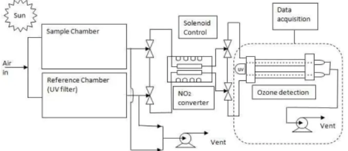
Fig. 1. Schematic of the MOPS. Equal air flows pass through the two chambers exposed to sunlight. The sample chamber passes so-lar ultraviolet light while the reference chamber has a film covering that blocks it. NO2converter cells enable the detection of NO2+ O3 by the dual-channel UV-absorption O3monitor.
continuously and yields the net rate of ozone production. This paper discusses the MOPS, its concept, operation, test-ing, and initial measurements at the Pennsylvania State Uni-versity.
2 Experimental methods
2.1 Principles of a direct ozone production measurement
The measurement of ozone production sensor (MOPS) has three components: two environmental chambers continu-ously exposed to solar radiation, a nitrogen dioxide-to-ozone conversion unit, and a modified ozone analyzer. A schematic of the instrument is shown in Fig. 1.
The sample chamber’s Teflon walls transmit solar ultravi-olet light so that the air in the sample chamber undergoes the same photochemistry that takes place in the ambient air. The reference chamber has a film that blocks radiation of wave-lengths less than 400 nm. As a result, the reference chamber limits the production of hydroxyl radicals (OH) generated by the photolysis of ozone followed by the reaction with water vapor. The photolysis of nitrous acid (HONO), a source of OH radicals, is also constrained. Similarly, the film on the reference chamber restricts the production of hydroperoxy radicals (HO2) produced by the photolysis of formaldehyde (HCHO). With radical chemistry eliminated, the only ozone in this chamber comes from the photostationary state (PSS) of the species NO, NO2, and O3. Since it is not possible to eliminate radical production without affecting NO2 photoly-sis near 400 nm, the PSS in the reference chamber tends to shift O3toward NO2. The total amount of ozone in the ref-erence chamber, therefore, is conserved in the form of NO2 plus O3.
Some of the ozone produced in the sample chamber re-acts with ambient NO and is partitioned into NO2according to the NOx PSS. At the same time, differences in the NO2 photolysis in the two chambers could cause the partitioning
of ozone and NO2in the two chambers to be different. The difference, nevertheless, between the total sum NO2+O3 in the sample chamber minus the sum in the reference cham-ber cancels out the PSS component of ozone production and yields only the component associated with the production of new ozone by radical chemistry.
The strategy, therefore, is to determine the differential of the sum O3+NO2 between the two chambers and divide it by the exposure time,τ, of the air inside them by means of Eq. (3) to determine the ozone production rate.
P (O3)=1O3/τ (3)
P(O3) is the net chemical ozone production,1O3is the difference in O3+ NO2 between the sample and reference chamber after the NO2has been converted into O3.
2.2 Technical details of MOPS
Air is sampled by both chambers through a common short Teflon inlet. The flow is split equally between the two cham-bers, which are identical in size and flow characteristics.
Two hollow cylindrical aluminum frames (17.78 cm di-ameter and 45.752 cm long) serve as support for Teflon film (FEP, 0.05 mm thick) that is wrapped around the frames. The volume of the chambers is 11.3 L and the flow of ambient air through each chamber is 1.5 L/min. The inlets and outlets to the chambers are pieces of Teflon tubing 2.54 cm diameter and 6.35 cm long. The flow is induced by a pump located downstream of the chambers. The sample chamber is clear Teflon so the air inside is radiated by all the wavelengths of the solar radiation that occur in the atmosphere. The ref-erence chamber, made the same as the sample chamber, is covered with an Ultem film (polyetherimide, 0.25 mm thick) that removes sunlight at wavelengths less than 400 nm.
After the conversion of NO2 into O3has taken place, the MOPS uses a modified ozone monitor (Thermo Scientific, Model 49i) to obtain a differential measurement of the ozone between the two chambers. The main modification applied to the commercial dual channel ozone monitor is the re-moval of the ozone scrubber. By doing so the ozone dif-ferential monitor receives a continuous supply of sample air from the sample chamber and reference air from the refer-ence chamber and detects the ozone differential in ppbv. Ad-ditionally, the temperature of the two UV absorption cells in the ozone monitor was stabilized by an aluminum block that was clamped tightly around the two absorption cells.
To account for the possible differences between the two photolytic conversion cells in the conversion unit, the flows of sample and reference air switch photolytic conversion cells every 5 min. To switch flows, the instrument has two pairs of solenoid valves. The first pair is located between the chambers and the conversion cells. The second pair of solenoid valves works synchronously with the first pair and is located between the conversion cells and the ozone moni-tor. In this way, the sample channel in the ozone instrument always measures the ozone from the sample chamber. The final reading is obtained as an average of the ozone differ-ential measured with each of the photolytic conversion cells switched to the sample chamber, giving an instrument time constant of twice 5 min, or 10 min.
The instrument uses a LabVIEW application for data ac-quisition and solenoid control. This application acquires additional information such as the temperature inside the MOPS chambers and the ambient NOxmixing ratios that are measured by a NO-NO2-NOxanalyzer (Thermo Scientific, Model 42C) that samples air near the MOPS.
2.3 MOPS characterization
The quantitative measurement of ozone production depends on the following factors: knowing the residence time in the chambers; having the atmospheric ozone production occur-ring in the sample chamber but not the reference chamber; measuring accurately the differences in the sum of O3 and NO2; and having all photochemistry that does not produce ozone but can affect the sum of O3and NO2be the same in the two chambers so that the differential measurement is not biased.
2.3.1 Mean exposure time
The ozone production measurement depends linearly on the exposure time. For a flow of 1.5 L/min through each 11.3 L chamber, the mean exposure time would be 7.5 min for a per-fect plug flow. Ideally, the aim is to have plug flow so that the time spent in the chamber is the same for every air molecule. The mean exposure time in the MOPS chambers was de-termined by adding a short pulse of ozone to the chambers and then monitoring the ozone at the exit. The pulse
ex-Fig. 2. Normalized mean ozone pulse for a series of four pulse experiments. A 20-s O3pulse was added at time = 0 s and O3was monitored at the output of the chamber. The pulses are normalized so that the peak value is 0.975.
periment not only helps determine the mean exposure time but also helps diagnose the type of flow inside the chambers. A normalized mean ozone distribution for a series of four pulses is shown in Fig. 2. The mean time obtained through this method is 5.8±0.3 min (95%,N= 4).
In addition to the pulse experiment, reactions with known amounts of ozone and excessα-pinene and ethene were per-formed independently. The decay of ozone was monitored over time until it decreased to a steady value greater than zero. This steady-state ozone value represents the average concentration remaining from ozone that has experienced re-action times distributed according to the distribution function depicted in Fig. 2. For example, while more ozone experi-enced 130 seconds of reaction than ozone did for any other time, some ozone experienced reaction for 1000 seconds or more. The mean ozone mixing ratio is equal to the integral of the normalized mean pulse distribution multiplied by the ex-ponential decay of ozone. The calculated mean ozone ratios agree to within 10% of the observed steady-state ozone that results from the reaction withα-pinene or ethene. The mean time was then calculated using the mean ozone mixing ratio, the initial ozone mixing ratio, and the rate coefficients. This calculated time agrees with the time required for the reac-tions to achieve steady state to within 5%. Finally, this same calculated time agrees with the time from the pulse experi-ment to within 10%.
uneven mixing that yield the tail of ozone distribution. The bulk of the ozone molecules, however, leave the chamber at a mean time of 5.8±0.3 min.
2.3.2 Radical abundances inside the chambers
One of the potential biases associated with the measurement of the rate of ozone production involves the abundances of the radicals OH, HO2, and RO2 inside the chambers. The radical abundances in the sample chamber should be the same as in the atmosphere, while the OH and HO2 abun-dances in the reference chamber should be zero. Because ozone is produced by the reaction of HO2and RO2radicals with NO, as shown in Eq. (1), an effective way to determine to what extent the proposed technique yields a quantitative measurement of ozone production is to compare the radical abundances inside the MOPS chambers with respect to the abundances in a controlled environment.
The strategy to determine radical loss was to create an ar-tificial atmosphere in an environmental chamber and mea-sure OH and HO2 in it. The sample chamber was placed in this artificial atmosphere and the radical concentrations were measured. The same procedure was followed with the reference chamber. A final measurement of OH and HO2 radicals in the empty artificial atmosphere was obtained to confirm the initial measurement of radicals. This experi-ment was completed by flowing air with 60 ppbv of ozone and 40% of relative humidity into an environmental chamber consisting of a 100 L Teflon FEP film bag with metal end-plates and exposing it to external ozone-free mercury lamps to produce OH and HO2and black lights to set the NOx pho-tostationary state. The OH and HO2radicals were measured with the Ground-based Tropospheric Hydrogen Oxides Sen-sor (GTHOS) (Faloona et al., 2004), which was attached to one of the ends of the large environmental chamber. The GTHOS sampling flow was 1 L/min, similar to the flow in MOPS. GTHOS sampled air directly from the artificial atmo-sphere and then from each MOPS chamber when they were placed inside the environmental chamber.
The HO2 radical abundance found in the MOPS sam-ple chamber agreed with the abundance in the artificial at-mosphere to within 5%. In the reference chamber (Ultem coated), the abundance of HO2radicals decreased to less than 10% of its initial value. RO2was not measured, but because RO2has reactions similar to those for HO2, it is likely that the behavior of RO2is similar to the observed behavior of HO2. The abundance of OH in the clear chamber was half of the abundance in the artificial atmosphere. The decrease in OH and no change in HO2indicate that the HOxproduction is the same as in the artificial atmosphere but the sample cham-ber may contain some additional OH loss. This difference in OH radicals, however, does not impact the rate of ozone production, as it can be observed in Eq. (1). In the reference chamber, the OH abundance decreased to virtually zero, as expected. These results indicate that the ozone-producing
photochemistry in the sample chamber is similar to that in the artificial atmosphere while the ozone producing photo-chemistry in the reference chamber is reduced to less than 10% of ambient.
2.3.3 Measurement of photolysis frequencies
In addition to these radical measurements, radiometric mea-surements were made in both chambers. The photolysis fre-quencies of the species NO2, O3, and HONO were measured using a Scanning Actinic Flux Spectroradiometer (SAFS) by B. Lefer at the University of Houston (Shetter and Muller, 1999; Shetter et al., 2002). The measurements were per-formed on a sunny day, 14 May 2009, at noon on the roof of the Moody Towers at the University of Houston.
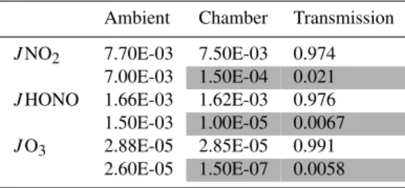
The blockage of UV light by the Ultem film in the ref-erence chamber was assessed by comparing the ambient ra-diometric measurements against the measurements obtained inside the reference chamber. A similar measurement and comparison were performed for the clear sample chamber. The results for the sample and reference chambers are shown in Table 1. When the radiometer was introduced in the ref-erence chamber coated with Ultem film, the photolysis fre-quencies for O3, NO2, and HONO dropped to less than 2% of the ambient values. In contrast, the photolysis frequencies measured inside the sample chamber remained within 3% of ambient values. These results confirm the radical measure-ments performed in the MOPS chambers and support the va-lidity of the technique in terms of restricting radical forma-tion in the reference chamber while conserving radical pho-tochemistry in the sample chamber.
2.3.4 NO2conversion efficiency
The conversion efficiency of the photolytic converter unit was tested for different levels of NO2 and is shown in Ta-ble 2. These results indicate that for most atmospheric abun-dances of NO2the efficiency of the conversion unit is 88% or higher. The conversion of NO2decreases as NO2increases because the rate of NO + O3→NO2+ O2increases to stay in photostationary state with the greater NO2 photolysis rate, thus shifting the NOx photostationary state away from O3 and toward NO2. At 88% conversion efficiency, the calcu-lated photolysis rate from the exponential decay of NO2is 0.09 to 0.1 s−1. In contrast, a typical atmospheric value for the NO2 photolysis frequency is 0.008 s−1 at midday on a sunny day.
Table 1. Measurement of photolysis frequencies,J (s−1), in the ambient air and the MOPS chambers. The shaded areas indicate photolysis frequencies measured inside the reference chamber (Ul-tem coated). Clear areas in the second and third columns correspond to measurements inside the sample chamber (clear). The last col-umn shows the transmission of chamber measurements with respect to the ambient.
Ambient Chamber Transmission
JNO2 7.70E-03 7.50E-03 0.974
7.00E-03 1.50E-04 0.021
JHONO 1.66E-03 1.62E-03 0.976
1.50E-03 1.00E-05 0.0067
JO3 2.88E-05 2.85E-05 0.991
2.60E-05 1.50E-07 0.0058
Table 2. Percentage of NO2converted to ozone in the converter
unit cells for different levels of NO2.
NO2(ppb) % Conversion
17 88
25 83
45 77
75 66
125 58
concentrations chosen are representative of a polluted day in the morning, at noon, at the peak of temperature, and in the evening. The rate coefficients for the model were taken from the data published by the Jet Propulsion Laboratory (JPL) (Sander et. al, 2006).
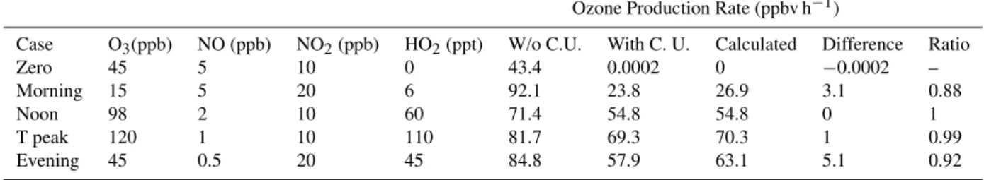
Table 3 presents the cases analyzed and results for the pro-duction of ozone with converter, without converter and the theoretical calculation of new ozone in ppbv h−1. The final columns are the difference between the MOPS measurement with the converter unit minus the theoretical calculation of new ozone and the ratio of the MOPS measurement with the converter unit to the theoretical calculation of new ozone.
The first case analyzed is the absence of production of new ozone, the concentration of HO2is zero and the photostation-ary state of ozone remains unperturbed. Consequently, the model theoretical calculation cancels out exactly the photo-stationary state and the ozone production is zero, as expected. The ozone that exits the reference chamber has partitioned mostly towards NO2. Without the ozone converter unit, the modified ozone analyzer would be unable to see the ozone in the form of NO2from the reference chamber and the result is an unrealistic ozone differential of 43.4 ppbv h−1of ozone production. Adding the NO2conversion in the converter unit minimizes the difference between the two chambers so the production of ozone is 0.0002 ppbv h−1.
Likewise, for the cases of ozone production due to the presence of HO2radicals, model calculations show that with-out the conversion unit the ozone differential between cham-bers is overestimated when compared against the theoretical calculation. By adding the NO2converter, the measurements become within 10% of theoretical values. The correction of the false signal is substantial such as the morning case in Ta-ble 3. Without the conversion unit, the ozone monitor would measure 92 ppbv h−1. The theoretical rate, however, corre-sponds to 26.9 ppbv h−1. The MOPS result with the con-verter is within 10% of the calculated new ozone. A highly efficient conversion unit, therefore, helps avoid the loss of ozone in the form of NO2and corrects a potential bias in the measurements.
2.3.5 Artefact due to high relative humidity and NO2 loss
Ideally, the only difference between the sample and refer-ence chambers is the photolysis in the sample chamber that enables ozone production. All other characteristics should be the same, including flows, relaxation towards NOx pho-tostationary state, and wall effects, so that any changes they induce in either ozone or NO2 cancel out in the differential ozone measurement. Thus, studies were devised to examine possible differences between the two chambers.
The wall loss of O3found in the MOPS chambers is less than 3%. For NO, the losses are less than 1%. The wall losses of these two species were not found to be a potential interference with the measurement.
The wall loss of NO2in the MOPS chambers was found to be significant for high relative humidity cases and for dif-ferences in relative humidity in the two chambers. This loss was studied by preparing NO2mixtures with air and varying the relative humidity. During these experiments, as relative humidity increased, the concentration of measured NO2 de-creased in a nonlinear fashion. For relative humidity higher than 50%, more NO2was removed as the relative humidity became higher. Previous research demonstrates that the up-take of water on a Teflon surface is about three times as much at 70% relative humidity as it is at 50% (Svensson et al., 1981). This condition of the Teflon surface has been proven to have an impact on the rate at which NO2 is removed at different relative humidities, resulting in nitric acid (HNO3) formation and HONO off-gassing (Wainman et al., 2001). The experiments performed with the MOPS chambers con-firm these findings.
Table 3.Model results for ozone production (ppbv h−1) without converter unit (W/o C.U.), with converter unit (With C.U.), and theoretically calculated. The last columns are the difference between calculated production rates and modeled results with the converter unit and the ratio of the model results with the converter unit to the calculated ozone production rate. The residence time in the chambers is 5.8 min while the residence time in the converter cells is 103 seconds. The photolysis frequency inside converter is 0.09 s−1. The photolysis frequency in the atmosphere is 0.008 s−1at noon. For the morning and evening cases,JNO2was assumed to be half of the noon value.
Ozone Production Rate (ppbv h−1)
Case O3(ppb) NO (ppb) NO2(ppb) HO2(ppt) W/o C.U. With C. U. Calculated Difference Ratio
Zero 45 5 10 0 43.4 0.0002 0 −0.0002 –
Morning 15 5 20 6 92.1 23.8 26.9 3.1 0.88
Noon 98 2 10 60 71.4 54.8 54.8 0 1
T peak 120 1 10 110 81.7 69.3 70.3 1 0.99
Evening 45 0.5 20 45 84.8 57.9 63.1 5.1 0.92
chamber is high, close to 80%, the NO2 removal is about 7 ppbv. This uneven NO2 removal causes a differential of about 6 ppb of NO2, which represent a false ozone produc-tion signal as high as 60 ppbv h−1. This false background correlates with anomalous signals that were observed during evenings in Houston Texas in which the relative humidity of the air jumped suddenly to high values.
An additional test was performed to ensure that the anoma-lies are actually associated with relative humidity. Air con-taining 60 ppbv of ozone, 60 ppbv of NO2and 94% relative humidity was prepared and sampled by the MOPS. The refer-ence chamber was heated with an infrared lamp to decrease its relative humidity without altering the absolute humidity of the air flow. As the relative humidity in the sample cham-ber became higher, there was a negative value for the ozone differential due to NO2removal.
The relative humidity can be different in the MOPS cham-bers due to differences in temperature in the two chamcham-bers. This difference is caused by the UV blocking film (Ultem) that covers the reference chamber. At the temperture peak during a hot summer day, the temperature in the clear sample chamber was as much as 5◦C above the ambient tempera-ture. The reference chamber was warmer than the sample chamber by another∼6◦C, thus up to 11◦C above the am-bient temperature for the warmest cases. These temperature differences cause little difference for the ozone production rates, since the rate coefficients of the reactions of HO2and RO2with NO have at little temperature dependence. How-ever, these temperature differences do translate into differ-ences in relative humidity between the two chambers.
During daytime, the higher-than-ambient temperatures in-side the MOPS chambers caused the relative humidity to be much less than 50%. Experimental data indicate that for the most extreme daytime cases, which occur in the early morn-ing, the interference due to NO2 removal can introduce a loss of about 1 ppbv out of 7 ppbv observed, or a 14% error, for the ozone differential. After early morning, the relative humidity decreases as the solar radiation intensifies and the
artefact error becomes insignificant. Later in the evening or at night, however, the artefact can sometimes affect the mea-surements.
When the ambient temperature decreases in the evening, the relative humidity of the air increases. If the relative hu-midity is high but the same in both chambers, then any NO2 removal on the Teflon film surfaces and HONO off-gassing will mostly cancel out in the differential O3+ NO2 measure-ment. However, it is possible that relative humidity differ-ences in the two chambers can cause the NO2 removal and HONO off-gassing to be different in the two chambers. Thus, high relative humidity can introduce an artefact in the MOPS data.
With the current version of MOPS, therefore, we consider as valid only the data collected when the relative humidity is below 50%. This condition is for the inside of the chambers and not for the ambient air. In daytime, the temperature in-side the chambers is higher than ambient by 5–11◦C, which
makes the relative humidity inside the chambers drop about 25% with respect to ambient. Hence, the MOPS can measure ozone production without introducing an artefact in the mea-surements at ambient relative humidities as much as 75% as long as the relative humidity inside the chambers stays below 50%. Fortunately, the relative humidity inside the chambers is lower than 50% for much of the daytime conditions under which ozone production is greatest, so that the current ver-sion of MOPS can measure ozone production without arte-facts during these polluted conditions.
2.3.6 Sensitivity, time constant and absolute uncertainty
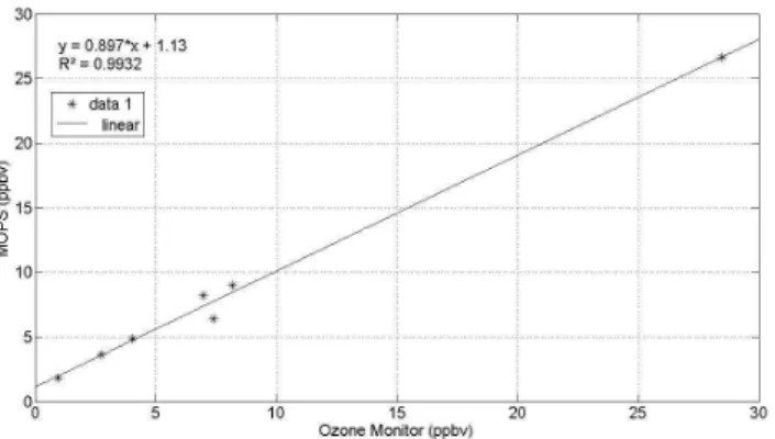
Fig. 3. Ozone differences seen by MOPS as a function of differ-ences seen by a Thermo Scientific 49i ozone monitor.
the level of sensitivity needed to measure urban ozone pro-duction can be done using the chemical propro-duction terms of Eq. (1) with atmospheric values for the species NO, HO2and RO2. For example, for conservatively low levels of pollutants such as 10 pptv for the sum [HO2+ RO2], 0.5 ppbv for [NO], and an effective rate coefficient of approximately 5×10⁻¹² (cm3molecules−1s−1), the rate of ozone production is ap-proximately 2.1 ppbv h−1. For highly polluted conditions, the ozone production rate can be in the range of 50 ppbv h−1. So, although the current MOPS is not sensitive enough to detect ozone production rates in the remote atmosphere, the MOPS detection limit of 0.67 ppbv h−1for the 10-min aver-age is sufficient to measure even low ozone production rates in urban and suburban air. The signal-to-noise ratio during the ozone production maximum is typically 20–30.
The main sources of uncertainty in the measurement of ozone production are the accuracy of the ozone differen-tial measurement and the uncertainty in the determination of mean exposure time. The accuracy of the MOPS ozone dif-ferential measurement was determined experimentally. Two ozone mixtures were prepared and their concentrations were measured using an ozone monitor (Thermo Scientific 49i). The difference in mixing ratios between the two mixtures was determined with the same ozone monitor without the ozone scrubber. As a next step, the same two ozone mix-tures were connected to the MOPS instrument in its operating mode. Figure 3 shows the ozone difference seen by MOPS as a function of the difference seen by the ozone monitor. The slope of the line is 0.90 and the mean of the ratio of the MOPS differential relative to the ozone monitor differ-ential is 1.22±0.31 (95%, N= 7). Thus, the uncertainty in the differential ozone measurement is approximately±25% (95%, N= 7). The uncertainty in the mean exposure time was obtained from the estimate of error in the pulse exper-iments and reaction experexper-iments and is±5%. The uncer-tainty introduced by differences in relative humidity is±14% for the early morning data. Other factors, such as the tem-perature difference between the sample and reference
cham-bers and ambient, contribute additional estimated uncertainty of ±10%. Thus, the absolute uncertainty (95% confidence level) of the current MOPS measurement is±30% for day-time operating conditions and±35% for data that could be affected by relative humidity such as in the early morning.
3 Test results
The first version of the MOPS instrument was tested on the University Park campus of the Pennsylvania State University in the late summer of 2008. The preliminary tests were per-formed on the roof of Walker Building, 30 m above one of the main streets in State College, PA. The air in this location corresponds to a rural background atmosphere disturbed by spikes of pollution from the traffic on the road below during rush hour.
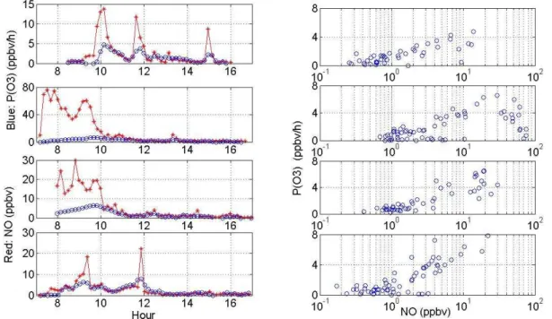
Figure 4 shows the data collected during 1 to 4 Septem-ber 2008. From the shape and magnitude of some of the NO spikes, it is evident that the MOPS was sampling fresh emis-sion plumes coming from vehicles on the main road. The ozone production rate follows NO, peaking at the same time, in particular for 1 and 4 September. These two days are char-acterized by similar NO emission peaks. 2 September was characterized by a plume of emissions with very high NO concentrations. In this case the ozone production was rather low when the NO was the highest, above 30 ppbv. These plots showed early evidence of the existence of a correla-tion betweenP(O3) and NO for these particular conditions, although not enough ancillary meaurements, particularly of radicals, were made to draw conclusions (Ren et al., 2003). These results, however, do indicate that this instrument could potentially clarify the discrepancies in the calculated ozone production rates from measured and modeled HO2.
These first tests demonstrate the feasibility of the MOPS technique. The instrument responded physically to the pres-ence of solar radiation and ozone precursors and yielded rates of ozone production in ranges that are within expected values for a polluted rural environment. In addition to being able to collect ambient measurements, these preliminary studies show that the MOPS can be used to investigate further the correlation betweenP(O3) and NO by adding precursors to the ambient air through both chambers and observing the ef-fect on the production of ozone.
4 Conclusions
Fig. 4. Rates of ozone production measured on the campus of the Pennsylvania State University during 1 to 4 September 2008. The left column contains time series forP(O3) (blue circles) and NO (red stars) for every day starting on Sep 1 and ending on 4 September 2008.
The right column is the correlation between measuredP(O3) and ambient NO.
virtually not present in the reference chamber. These condi-tions ensure that the differential of ozone between chambers yields the measurement of the ozone produced by reactions between peroxy radicals and NO only. The tests performed on the current version of MOPS, therefore, indicate that the instrument works correctly for the detection of ozone pro-duction rates.
The detection limit of the current MOPS is 0.67 ppbv h−1 for the 10-min average data. This limit can be lowered by improving the sensitivity of the detection cells. A better sen-sitivity of detection would enable the use of smaller sample and reference chambers and shorter exposure times.
At the 95% confidence level, the absolute uncertainty of the instrument is 30% for measurements not affected by rel-ative humidity. For early morning data, the uncertainty in-creases to 35% at the same confidence level. The uncertain-ties in the measurement can be reduced, in part, by minimiz-ing wall effects that cause NO2losses. One possibility is to improve the flow pattern in the chambers so that the motion resembles more closely plug flow. Methods of improving the flows are now being studied.
The MOPS is an inexpensive instrument that, when added to air quality networks, would greatly enhance the under-standing of ozone pollution issues in urban and suburban environments. The MOPS retrieved the first experimental plots P(O3) vs. NO in early September 2008. The direct measurement of ozone production rates can contribute to the improvement of air quality regulations. Furthermore, the MOPS technique can be used to address the discrepancy
between modeled and measured HO2. A first step towards elucidating these discrepancies would be the deployment of the MOPS instrument along with the Ground-based Tropo-spheric Hydrogen Oxides Sensor (GTHOS) to collect data over a period of time and compare the ozone production rates calculated from modeled and measured HO2. The instrument can also be used to quantify the importance of locally pro-duced ozone versus transported ozone. Finally, sensitivity analysis can be performed with the MOPS by adding NO to the ambient air to provide an indicator of NOxsensitivity to ozone production.
Acknowledgements. The authors thank the College of Earth and Mineral Sciences at the Pennsylvania State University for the Miller Faculty Fellowship, which provided graduate student support for M. C. and funds for the fabrication of MOPS. NSF grant ATM-0209972 supported the initial development of MOPS. We also thank B. Lefer and J. Flynn for measuring the photolysis frequencies in May 2009 in Houston, D. van Duin and X. Ren for help with the radical chamber studies, and K. Biddle and the EMS machine shop for MOPS fabrication help.
References
Faloona, I. C., Tan, D., Lesher, R. L., Hazen, N. L., Frame, C. L., Simpas, J. B., Harder, H., Martinez, M., Di Carlo, P., Ren, X., and Brune, W. H.: A laser induced fluorescence instrument for detecting tropospheric OH and HO2: Characteristics and calibra-tion, J. Atmos. Chem., 47, 139–167, 2004.
Finlayson-Pitts, B. J. and Pitts Jr., J. N.: The chemical basis of air quality: Kinetics and mechanism of photochemical air pollution and application to control strategies, Advances in Environmental Science and Technology, edited by: Pitts Jr., J. N. and Metcalf, R. L., New York, USA, Wiley-Interscience Publication, 75–162, 1977.
Forster, P., Ramaswamy, V., Artaxo, P., Berntsen, T., Betts, R., Fa-hey, D. W., Haywood, J., Lean, J., Lowe, D. C., Myhre, G., Nganga, J., Prinn, R., Raga, G., Schulz, M., and Van Dorland, R.: Changes in Atmospheric Constituents and in Radiative Forc-ing. In: Climate Change 2007: The Physical Science Basis. Con-tribution of Working Group I to the Fourth Assessment Report of the Intergovernmental Panel on Climate Change, edited by: Solomon, S., Qin, D., Manning, M., Chen, Z., Marquis, M., Av-eryt, K. B., Tignor, M., and Miller, H. L., Cambridge University Press, Cambridge, United Kingdom and New York, NY, USA, 150–152, 2007.
G´ego, E., Porter, P. S., Gilliland, A., and Rao, S. T.: Observation-Based assessment of the impact of Nitrogen Oxides emissions reductions on ozone air quality over the Eastern United States, J. Appl. Meteor. Clim., 46, 994–1008, 2007.
Gery, M. W., Whitten, G. Z., Killus, J. P., and Dodge, M. C.: A photochemical kinetics mechanism for urban and regional scale computer modeling, J. Geophys. Res., 94, 12925–12956, 1989. Haagen-Smit, A. J., Bradley, C. E., and Fox, M. M.: Ozone
forma-tion in photochemical oxidaforma-tion of organic substances, Ind. Eng. Chem., 45, 2086–2089, 1953.
Ho, W. C., Hartley, W. R., Myers, L., Lin, M. H., Lin, Y. S., Lien, C. H., and Lin, R. S.: Air pollution, weather, and associated risk fac-tors related to asthma prevalence and attack rate, Environ. Res., 104, 402–409, 2007.
Kanaya, Y., Cao, R., Akimoto, H., Fukuda, M., Komazaki, Y., Yokouchi, Y., Koike, M., Tanimoto, H., Takegawa, N., and Kondo, Y.: Urban photochemistry in central Tokyo: 1. Ob-served and modeled OH and HO2radical concentrations during
the winter and summer of 2004, J. Geophys. Res., 112, D21312, doi:10.1029/2007JD008670, 2007.
Kemball-Cook, S., D. Parrish, T. Ryerson, U. Nopmongcol, J. John-son, E. Tai, and Yarwood, G.: Contributions of regional transport and local sources to ozone exceedances in Houston and Dallas: Comparison of results from a photochemical grid model to air-craft and surface measurements, J. Geophys. Res., 114, D00F02, doi:10.1029/2008JD010248, 2009.
Kleinman, L. I., Daum, P. H., Lee, Y. -N., Nunnermacker, L., Springston, S. R., Newman L., Weinstein-Lloyd, J., and Sillman, S.: Dependence of ozone production on NO and hydrocarbons in the troposphere, J. Geophys. Res., 24, 2299–2302, 1997. Kleinman, L. I., Daum, P. H., Lee, Y.-N., Nunnermacker, L., and
Springston, S. R.: Ozone production efficiency in an urban area, J. Geophys. Res., 107(D23), 4733, doi:10.1029/2002JD002529, 2002.
Kleinman, L. I.: The dependence of tropospheric ozone production rate on ozone precursors, Atmos. Environ., 39, 575–586, 2005.
Logan, J. A., Prather, M. J., Wofsy, S. C., and McElroy, M. B.: Tropospheric Chemistry: A global perspective, J. Geophys. Res., 86, 7210–7254, 1981.
Madden, M. C. and Hogsett, W. E.: A Historical Overview of the Ozone Exposure Problem, Human Ecol. Risk Assess., 7(5), 1121–1131, 2001.
Martinez, M., Harder, H., Kovacs, T. A., Simpas, J. B., Bassis, J., Lesher, R., Brune, W. H., Frost, G. J., Williams, E. J., Stroud, C. A., Jobson, B. T., Roberts, J. M., Hall S., R., Sheter, E., Wert, B., Fried, A., Alicke, B., Stutz, J., Young,
V. L., White A. B., and Zamora, R. J.: OH and HO2
concen-trations, sources, and loss rates during the Southern Oxidants Study in Nashville, Tennessee, summer 1999, J. Geophys. Res., 108(D19), doi:10.1029/2003JD003551, 2003.
National Research Council (NRC): Rethinking the ozone problem in urban and regional air pollution, Natl. Acad. Press, 109–186, 1991.
Ren, X., Harder, H., Martinez, M., Lesher, R., Oliger, A., Simpas, J., Brune, W., Schwab, J., Demerjian, K., He, Y., Zhou, X., and
Gao, H.: OH and HO2 Chemistry in the urban atmosphere of
New York City, Atmos. Environ., 37, 3639–3651, 2003. Ren, X. R., Harder, H., Martinez, M., Faloona, I. C., Tan, D.,
Lesher, R. L., Di Carlo, P., Simpas, J. B., and Brune, W. H.: In-terference testing for atmospheric HOxmeasurements by
laser-induced fluorescence, J. Atmos. Chem., 47, 169–190, 2004. Sander, S. P., Friedl, R. R., Golden, D. M., Kurylo, M. J., Moortgat,
G. K., Wine, P. H., Ravishankara, A. R., Kolb, C. E., Molina, M. J., Finlayson-Pitts, B. J., Huie, R. E., and Orkin, V. L.: Chemical kinetics and photochemical data for use in atmospheric studies, Evaluation Number 15, JPL Publication 06–2, NASA Jet Propul-sion Laboratory, Pasadena, CA, USA, 2006.
Shetter, R. E. and M¨uller, M.: Photolysis frequency measurements using actinic flux spectroradiometry during the PEM-Tropics mission: Instrumentation description and some results, J. Geo-phys. Res., 104, 5647–5661, 1999.
Shetter, R. E., Cinquini, L., Lefer, B. L., Hall, S. R., and Madronich, S.: Comparison of airborne measured and calculated spec-tral actinic flux and derived photolysis frequencies during the PEM Tropics B mission, J. Geophys. Res., 108(D2), 8234, doi:10.1029/2001JD001320, 2003.
Shirley, T. R., Brune, W. H., Ren, X., Mao, J., Lesher, R., Carde-nas, B., Volkamer, R., Molina, L. T., Molina, M. J., Lamb, B., Velasco, E., Jobson, T., and Alexander, M.: Atmospheric oxi-dation in the Mexico City Metropolitan Area (MCMA) during April 2003, Atmos. Chem. Phys., 6, 2753–2765, 2006,
http://www.atmos-chem-phys.net/6/2753/2006/.
Sillman, S.: Tropospheric ozone: the debate over control strategies, Ann. Rev. Ener. Environ., 18, 31–53, 1993.
Sillman, S.: The use of NOy, H2O2, and HNO3as indicators for ozone-NOx-hydrocarbon sensitivity in urban locations, J.
Geo-phys. Res., 100, 14175–14188, 1995.
Svensson, R., Ljungstrom, E., and Lindqvist, O.: Kinetics of the reactions between nitrogen dioxide and water vapor, Atmos. En-viron., 21, 1529–1539, 1987.
Taubman, B. F., Thompson, A. M., Fuentes, J. D., Joseph, E., Michaels, S. M., Robjhon, M., and Piety, C. A.: The Mid-Atlantic low level jet and its implications for air quality, J. Geo-phys. Res., doi:2008JD009798, submitted, 2009.
efficiency to asses ozone sensitivity to hydrocarbons and NOx: 1.
Local Indicators of Odd Oxygen Production sensitivity, J. Geo-phys. Res., 105, 9213–9225, 2000.
Tonnesen, G. S. and Dennis, R. L.: Analysis of radical propagation efficiency to asses ozone sensitivity to hydrocarbons and NOx:
2. Long lived species as indicators of ozone concentration sensi-tivity, J. Geophys. Res., 105, 9227–9241, 2000.