Just-in-Time Compilation-Inspired Methodology for
Parallelization of Compute Intensive Java Code
GHULAM MUSTAFA*, WAQAR MAHMOOD**, AND MUHAMMAD USMAN GHANI* RECEIVED ON 02.09.2015 ACCEPTED ON 14.12.2015
ABSTRACT
Compute intensive programs generally consume significant fraction of execution time in a small amount of repetitive code. Such repetitive code is commonly known as hotspot code. We observed that compute intensive hotspots often possess exploitable loop level parallelism. A JIT (Just-in-Time) compiler profiles a running program to identify its hotspots. Hotspots are then translated into native code, for efficient execution. Using similar approach, we propose a methodology to identify hotspots and exploit their parallelization potential on multicore systems. Proposed methodology selects and parallelizes each DOALL loop that is either contained in a hotspot method or calls a hotspot method. The methodology could be integrated in front-end of a JIT compiler to parallelize sequential code, just before native translation. However, compilation to native code is out of scope of this work. As a case study, we analyze eighteen JGF (Java Grande Forum) benchmarks to determine parallelization potential of hotspots. Eight benchmarks demonstrate a speedup of up to 7.6x on an 8-core system.
Key Words: Just-in-Time Compilation, Loop Level Parallelization, Multicore System, Runtime Analysis, Java Virtual Machine.
* Department of Computer Science & Engineering, University of Engineering & Technology, Lahore. ** Al-Khwarizmi Institute of Computer Science, University of Engineering & Technology, Lahore.
re-compiling [7]. A drawback of static auto-parallelizing compilers is that dynamic execution state of application is not available during compilation. On the other hand, dynamic compilers and run time systems could exploit characteristics of running code in parallelization process.
Runtime systems parallelize applications either speculatively [8-11] or non-speculatively [12-15]. In speculative parallelization, potential parallel tasks are assumed to have no dependences and run using either TLS (Thread Level Speculation) [16] or transactional memory [17]. Results are not committed if the system detects dependence violation(s). Runtime system ensures
1.
INTRODUCTION
the resolution of dependences by squashing and re-running some of parallel tasks. This is a best effort approach that exploit parallelism if possible, otherwise code is run sequentially. In non-speculative parallelization paradigms, dependences are analyzed first and code is usually transformed to expose hidden parallelism. Parallel tasks are synchronized properly to preserve sequential semantic, and avoid dead/live locks and data races. However, both cases have their own challenges.
JIT systems are typically used to facilitate dynamic compilation of binary code during execution [19-21]. In case of Java, inefficiency of interpreted Java code stimulated the renaissance of JIT technologies [19]. Java (source code) compiler converts source code into bytecode which is stored in class file format. Classes are loaded in JVM (Java Virtual Machine) on-demand and bytecode instructions are interpreted by JVM. For JIT compilation, JVM profiles running applications to select most frequently called and/or most time consuming code regions as hotspots. JIT compiler dynamically compiles hotspots to potentially optimized native code. Since JIT compilers can exploit runtime characteristics of applications, it is plausible to use JIT compilation infrastructure for parallelization.
Typically, majority of computer applications spend large amount of their runtime in the hotspots [22-23]. We observed that compute intensive hotspots have huge parallelization potential [22]. This work focus on a single goal: achieve whatever parallelism can be realized from sequential code without any effort on the part of exploring hidden parallelism. Being a best effort approach, it may improve scalability where it can exploit parallelism potential but in other cases it may not modify even a single loop. Using profiler feedback, compute intensive DOALL loops are selected from Java bytecode just as JIT compiler selects frequently executing code for native translation. We have two reasons for considering loop level parallelization in this context. First, we observed that by setting a threshold on application’s execution
time, we are left with only a few most time consuming methods [22]. For example, setting 90% threshold in JGF Crypt benchmark revealed that a single method consumed 90% time of the application [24]. Such cases are not suitable for method level parallelization even on dual core system. Similarly, JIT compilation infrastructure selects only few methods as hotspots. Method level parallelization determines potential parallelism by doing inter-procedural analysis of complete application. During inter-procedural analysis, if some non-hotspot method is found as a caller of hotspot(s), modifications will also be needed in the non-hotspot method. Eventually, we will be dealing with entire application and taking almost no advantage of JIT compilation infrastructure. In contrast, modifications applied at loop level remains local to the hotspot only. JIT compiler could produce parallel native code transparently.
The paper is organized in following sections: Section 2 presents related work. Problem statement is formulated in Section 3 along with qualitative and quantitative features. Overall methodology is proposed in Section 4. Parallelization steps and implementation details are given in Section 5. Case studies and results are discussed in Section 6. Paper is concluded in Section 7.
2.
RELATED WORK
auto-parallelizing extensions for Java JIT compiler so that the compiler could find potentially parallelizable code and compile it for parallel execution on multicore CPU and GPGPU (General Purpose Graphic Processing Unit) [30]. However, code generation depends on RapidMind and GPU hardware [31]. Majority of other efforts on runtime parallelization focus on speculative execution and/or exploit method level parallelism [32-38].
3.
PROBLEM FORMULATION
Let an application calls Nm methods during execution and each method mj consists of k loops, where j > 1 and k > 0. Starting from main() method, j-1 other methods are typically called in hierarchical manner and inter-procedural relationships are represented as a call graph. Call graph is a directed graph G = <V, E>, where V is a finite set of vertices and E is a finite set of edges. Each vertex v∈V represents a method invocation and each edge
e∈E between a vertex pair (u,v) represents one or more
invocations of v by u (i.e. u→v). Static call graph is
constructed by source code browsing whereas dynamic call graph is obtained by profiling the running application. Sorted flat profile F is a list representation of dynamic call graph, where |F| = Nm. Typically, F also contains runtime
information like calls count, time consumption and percentage time consumption of each method. Percentage time consumption of a method is actually PC (Percentage Contribution) of method toward total execution time of application, where PC is defined as:
100 Appliction by the
Consumed Time
Total
Method by the Consumed Time
Net
PC
3.1
Percentage Contribution Threshold
TPC (Percentage contribution threshold) is the part of application run time (< 100%) that we want to be parallelized [22]
.
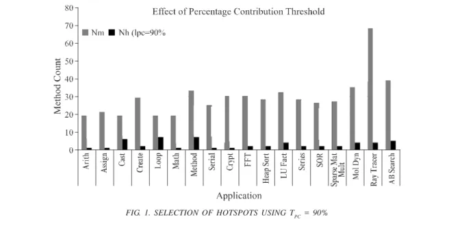
For example, setting TPC = 80% for an application means that we are interested in parallelizing only most time consuming methods (i.e. hotspots) that collectively consume 80% time of the application. Fig. 1 shows the effect of setting TPC = 90% for eighteen JGF application benchmarks [24], where Nh is the number of hotspots. It is obvious from Fig. 1 that majority of methods are shunt out because they collectively consume<10% time of the application. Analyzing and modifying these methods is likely to increase runtime overhead and may result in performance degradation compared to sequential code.
TPC facilitates the selection of hotspot methods. Next, we need to determine various characteristics of hotspot methods. We enumerate these characteristics in catalogs of qualitative and quantitative features of methods, as shown in Tables 1-2, respectively.
3.2
Qualitative Features of Methods
Qualitative features are binary variables to represent different characteristics of the method. Each qualitative feature indicates the presence (or absence) of a specific characteristic of a method, as described in Table 1. For example, LOOPY=0 means that the method does not contain loops. The idea of qualitative features is inspired by Nano-patterns that were proposed to characterize and classify Java methods [39]. Catalog of qualitative features is constructed by extended catalog of Nano-patterns from 17 to 32, and giving them compact and descriptive names. Previously, we used qualitative features to analyze thread level speculative parallelization potential at runtime [22]. We showed that binary features are very important decisive factors for runtime qualitative analysis of parallelization potential of methods. Qualitative features are generic in nature and could be used in any software reverse engineering and reengineering activity. We used some relevant features in this work.
3.3
Quantitative Features of Methods
Presence of a particular characteristic of method potentially necessitates the quantification of that characteristic. For example, if a method contains loops (i.e. LOOPY=1), we need to determine the number of single and nested loops. For this, we will observe the quantitative features f37 and f38 in Table 2. In Table 2, 15 quantitative features are cataloged to represent static and dynamic characteristics of a method. Static and dynamic characteristics are gathered by parsing classes at load time and profiling the running application, respectively. Qualitative and quantitative features abstract the general
purpose code characteristics to help in runtime code comprehension. In this work, we used only those features that are helpful in loop level parallelization. Each feature is determined by using a specific algorithm. For the sake of brevity, only two algorithms, related to determination of f37 and f38, are presented in section 4.2.
D
I Feature fITruethentheMethod…
f0 NO_ARGS Takesnoargumenst
f1 VALUE_ONSLY_ARG- Takesonlypass-by-valueargumenst
f2 REF_ONLY_ARGS Takesonlypass-by-referenceargumenst
f3 MIXED_ARGS Takesmixedanyargumenst
f4 ARRAY_ARGS Takesoneormorearrayargumenst
f5 NO_RET Returnsvoid
f6 VALUE_RET Returnspirmiitvevalue
f7 REF_RET Returnsreferencevalue
f8 STATIC si tsatci
f9 RECUR sirecurisve
f10 LOOPY containsatelatsoneloop
f11 NESTED_LOOPY containsatelatsonenetsedloops
f12 EXCEPT throwsexcepiton
f13 LEAF Hasnocalelemethod
f14 OBJ_C createsnewobjecst
f15 FIELD_R readscalssfeild(s)
f16 FIELD_W wrtiescalssfeild(s)
f17 TYPE_M usestypecasitng
f18 NO_BR hassrtaightilnecode
f19 LOCAL_R readslocalvaraibel(s)
f20 LOCAL_W wrtieslocalvaraibel(s)
f21 ARRAY_C createsnewarray(s)
f22 MDARRAY_C createsnewmutl-iDarray(s)
f23 ARRAY_R readsarray value(s)
f24 ARRAY_W wrties array value(s)
f25 THIS_R readsfeildvalue(s)oft'hi'sobject
f26 THIS_W wrtiesfeildvalue(s)oft'hi'sobject
f27 OTHER_R reads feildvalue(s)ofotherobjec(ts)
f28 OTHER_W wrties feildvalue(s)ofotherobjec(ts)
f29 SFIELD_R reads tsatcifeildvalue(s)
f30 SFIELD_W wrties tsatcifeildvalue(s)
f31 SAMENAME calslovelroadedmethod(s)
4.
PROPOSED METHODOLOGY
Proposed methodology transforms Java classes at load time and works in three phases. Overall work flow is shown in Fig. 2. In profiling phase, an application is test-run to get profiling data. Profiler output is fed back to JVM during actual run. Using a value of TPC (i.e. 90% in this paper),
top Nh hotspot methods are selected form the flat profile F which is sorted by PC in descending order. JVM class loader is hooked so that classes could be parsed and transformed at load time [22]. Each class is parsed and modified just before it is loaded by the JVM. In parsing phase, list of methods Lm of a class i is acquired to determine if it contains a hotspot. If a method mij is hotspot, it is parsed to generate (1) list of qualitative features (2) list of quantitative features (3) list of backward jumps LSL (4) IR tuples, and (5) instruction patterns. A list of nested loop LNL is then generated using the loops of LSL. In modification phase, a heuristic on call count (CC i.e. feature f46) of mij is used to determine the potential location of parallelizable loop(s). If CC<Nm and mij is LOOPY then potentially parallelizable loop(s) lies within mij otherwise lies within some caller of mij. This heuristic implies that if CC is significantly large, the time consumption of mij is not due to the loops in it but (potentially) it has been called within a loop of its parent method. In later case, parent of mij becomes a hotspot provided that it is LOOPY. In any case, we get a loop lijk. If lijk is DOALL, it is marked to be modified for parallel execution using the operations mentioned in modification phase of Fig. 2 and threading framework of section 4.4.
D
I Feature Descirpiton
f32 FIELDs #Non-tsatcifeildsaccessedinmethodbody
f33 SFIELDs #Statcifeildsaccessedinmethodbody
f34 CALLs #Methodcalslinthemethod
f35 JUMPS #Jumps j(umpinsrtucitons)inthemethod
f36 BRANCHES #Forwardjumps(branches)inthemethod
f37 SINGLELOOPS #Singelloopsinthemethod
f38 NESTEDLOOPS #Netsedloopsinthemethod
f39 ICOUNT #Insrtucitonsinthemethod
f40 LOOPICOUNT #Insrtucitonsintheloopbodeis
f41 STACKMAX Maximum tsack lsost(.ie. tsackszie)
f42 LOCALMAX #Localvaraibels i(ncludingargumenst)
f43 ARGS #Argumenstofthemethod
f44 TIME Timeconsumedbythemethod
f45 PC PercentageContirbuitonofthemethod
f46 CC CallCountoftheethod
TABLE 2. QUANTITATIVE FEATURES OF METHODS
4.1
Parallelization Criteria
There are two criteria for best effort parallelization of a loop.
Criterion-1: Hotspot Selection: Set TPC = 90% and select most time consuming methods that collectively consume 90% time of application, as hotspots.
Criterion-2: Loop Selection: If a hotspot has significantly high CC value (e.g. > Nm), then go to its calling method(s). In (any of) calling method, if the hotspot is called in a loop and the loop is DOALL, transform it for parallel execution.
(i) Otherwise, if the hotspot itself contains DOALL loop(s), transform it (them) for parallel execution.
(ii) In case of invalidation of (I) and (II), run unmodified sequential application.
4.2
Loop Profiling
Loop profiling is used to determine the features like SIMPLELOOPS and NESTEDLOOPS. In each hotspot, loops are detected by recording the backward jumps. Each backward jump is represented as quadruple <Offset, Target, Index, Stride>, where Offset is the offset of backward jump, Target is offset of the target label of backward jump, Index is the variable acting as loop index and Stride is the step size of loop iterations. All backward jumps are recorded during parsing phase. Each backward jump is a potential single loop. A backward jump is one whose target has already been visited [39], either in terms of labels or memory addresses. Labels are used in bytecode because exact memory addresses are not known in intermediate code. By constructing basic block level CGF (Control Flow Graph), we can classify a backward jump as a loop if its Target lies in one of the dominator blocks of the block that contains its Offset. A block d dominates a block b (i.e. d DOM b), if all paths from entry
block to bincluded. Also, DOM (b) denotes a set of all nodes that dominate b (including b itself).
Nested loops are determined by observing the organization of simple loops. If a loop lies exactly within another loop then we come up with a loop nest. For two simple loops li and lj if Offseti>Offsetj AND Targeti<Targetj then lj lies within li. So, there exist a 2-level nested loop instead of two single loops. In real world code, inner loops in a loop nest may appear in a variety of ways, as shown in Fig. 3. A loop nest could be represented as a loop tree to accommodate all possible organizations of inner loops. Root of tree represents the outer most loop and other nodes represent inner loops of root. The data associated with each node is the loop quadruple, a reference to its parent node and a list of references to its children nodes. Traversing nodes of a loop tree, we can represent nested loops as a 5-tuple <Offset, Target, Nest-Level, {Index-Vector}, {Stride-Vector}> where Offset is the offset of outer most loop, Target is offset of target label of outer most loop, Nest-Level is the height of loop tree,
(a) TRANSFORM_INTERNAL() METHOD OF JGF FFT BENCHMARK
(b) RUNITERS() METHOD OF JGF MOLDYN BENCHMARK. A LOOP FOREST IS IN
(c) MATGEN() METHOD OF LUFACT BENCHMARK
Vector is a list of indices of all loops in loop nest and Stride-Vector is a list of step sizes of all loop in loop nest. Generally, a loop forest containing single and/or multi-node tree(s), is constructed against each hotspot.
4.2.1 Algorithm for Identification of Single
Loops
Single loop detection algorithm is shown in Table 3. Let Si be the instruction stream of a method. During interpretation in a test run, each visited label l is added to a list of visited labels Lv. For each branch instruction b, if the branch’s target label lb has already been visited then b represents a backward jump. Let BlockA and BlockB are two basic blocks (as nodes) in CFG. If b∈block
Aand lb∈blockBand blockB∈ DOM (blockA), then b is a loop conditional. Prepare quadruple <Offset, Target, Index, Stride> against b and add to a list of single loops Lloop.
4.2.2 Algorithm for Loop Forest Construction
Once we get a list of single loops Lloop- using the algorithm shown in Figure 4, we can determine nested loops by using algorithm shown in Table 4. Considering each single loop ls∈L
loop as a node, loop tree Tl is constructed against each nested loop and added to a loop forest Fl. Depending upon the availability of loops, Fl could possibly be (1) empty (2)
containing single-node tree(s) only (3) containing multi-node tree(s), or (4) containing a mixture of single-multi-node and multi-node trees. At start the loop forest Fl is empty and a tree Tl is constructed using the first loop of Lloop as root node. Subsequent loops from Lloop are either added to an existing tree or cause the generation of new tree(s). An existing tree is re-adjusted if an outer loop comes after some inner loop(s) so that outer most loop is always the root node.
4.3
Loop Classification
Using feature f37 and f38, we can iterate on all loops to classify them. As we are only interested in parallelization of compute intensive DOALL loops (having arbitrary stride size), we select DOALL loops by observing potential inter-iteration data dependences. Data dependences are analyzed by recognizing instruction patterns corresponding to read/write of local variables, arrays elements, and class members of primitive and user-defined data types. In a DOALL loop, all memory access (instruction) patterns operate on independent memory locations in each iteration. As number of instruction patterns depends on instruction set size, we define an intermediate representation to reduce the (instruction) pattern processing cost.
Input: Si
Output: Lloop
FOR EACH instruction i
IF i == l THEN
Add l to Lv
END IF
IF i == b AND lb∈Lv THEN
Backward Jump found.
IF b∈ blockA AND
lb∈ blockB AND
blockB ∈ DOM (blockA)
THEN
Prepare Quadruple <Offset, Target, index, stride> Add <Offset, Target, index, stride> to Lloop
END IF END IF END FOR
Input: Lloop
Output: Fl
FOR EACH ls
∈
LloopIF Fl is empty THEN
Create a new tree rooted at ls, in Fl
ELSE Identify an existing Tl in Fl
IF Tl found THEN
IF ls is inner loop of root of Tl THEN
Insert ls to Tl at appropriate place
ELSE reorder Tl to make ls its root
END IF-ELSE
ELSE create a new tree rooted at ls, in Fl
END IF-ELSE END IF-ELSE END FOR TABLE 3. ALGORITHM TO IDENTIFY SINGLE LOOPS
TABLE 4. ALGORITHM TO CONSTRUCT LOOP FOREST. MULTI-NODE TREES IN THE FOREST REPRESENT
4.3.1 Intermediate Representation of
Bytecode Instructions
IR (Intermediate Representation) of bytecode instructions is defined to reduce instruction pattern count and potential pattern processing effort. If an instruction set contains n instructions. We might have to look for (n)p combinations to recognize an instruction pattern of length p. These combinations could be reduced if we reduce n by symbolically representing n instructions with m symbols, where m<n. For example, a subset of bytecode instructions {IADD, LADD, FADD, DADD} is used to perform arithmetic addition of two {integer, long-integer, floating–point, double-precision-floating-point} numbers, respectively. A high level IR symbol ADD could suffice to recognize any of these four instructions. Similarly, we can recognize entire instruction set using a smaller set of IR symbols. By defining IR symbols, we could represent ~200 bytecode instructions (i.e. n ≈ 200)
with 42 symbols (i.e. m = 42), as shown in Table 5. Labels are typically induced by compiler to facilitate control flow and demarcation of basic blocks. We consider LBL as part of IR symbols because labels are integral part of compiled code. As elaborated in next sub-section, presentation of instruction patterns in terms of IR symbols increases the occurrence frequency of instruction patterns. Using IR symbols, we have about five times (i.e. n/m) fewer choices at each
position in instruction pattern.
4.3.2 Recognition of Instructions Patterns
Compilers typically generate an instruction pattern against each source code statement. Java source compiler generates a stream of bytecode instructions which is interpreted by JVM. We recognize bytecode instruction patterns to distinguish memory accesses. The idea starts with the preparation of a catalog of ISA-specific fundamental instruction patterns. Each fundamental pattern consists of at least two instructions in a specific order and performs a smallest indivisible source level task e.g. “variable initialization”. Some instructions like INC or LV (Table 5) could independently perform an indivisible source level task
e.g. “j++;”. We enumerate such instructions as independent instructions. A pattern is an arrangement of two or more independent instructions. Figure 6 shows an inner loop from SORrun(…) method of JGF SOR benchmark [24], to elaborate instruction pattern recognition.
l o b m y
S Descirpiton BytecodeInsrtucitons
_ DoNothing NOP
C
L LoadContsant ACIOCONSNTS_TN_U4,LILC,OICNOSNT_S5T,_LMC1O,NICSOTN_0S,TL_C0O,INCSOTN_S1,TF_1C,OICNOSTN_S0T,_F2C,OICNOSNTS_1T,_3, W _ 2 C D L , W _ C D L , C D L , H S U P I S , H S U P I B , 1 _ T S N O C D , 0 _ T S N O C D , 2 _ T S N O C F V
L LoadValue ILOAD,LLOAD,FLOAD,DLOAD
R
L LoadReference ALOAD
A V
L LoadValue rfomArray IALOAD,LALOAD,FALOAD,DALOAD,BALOAD,CALOAD,SALOAD
A R
L LoadReferenceArrayValue AALOAD
V
S StoreValue ISTORE,LSTORE,FSTORE,DSTORE
R
S StoreReference ASTORE
A V
S StorepirmiitveArrayValue IASTORE,LASTORE,FASTORE,DASTORE,BASTORE,CASTORE,SASTORE
A R
S StoreReferenceArrayValue AASTORE
P
P Pop POP,POP2
P
D Duplciate DUP,DUP_X1,DUP_X2,DUP2,DUP2_X1,DUP2_X2
P
S SWAP SWAP
O
A ArtihmetciOperaiton IADD,LADD,FAIDDDIV,,DLADDIVD,,FIDSUIVB,,DLDSIUVB,I,RFESMUB,L,RDESMUB,F,IRMEMUL,,DLRMEUML,FMUL,DMUL,
O
L LogcialOperaiton INEG,LNEG,FNEG,DNEG,ISIHOLR,,LLSOHRL,,IISXHORR,,LLSXHORR,IUSHR,LUSHR,IAND,LAND, C
N
I Increment IINC
P 2
P Pirmiitve-PirmiitveCasitng I2L,I2F,I2D,L2,IL2F,L2D,F2,IF2L,F2D,D2,ID2L,D2F,I2B,I2C,I2S
P M
C Compare LCMP,FCMPL,FCMPG,DCMPL,DCMPG
1 F
I 1-ValueIFStatement IFEQ,IFNE,IFLT,IFGE,IFGT,IFLE
2 F
I 2-ValuesIFStatement IF_ICMPEQ,IF_ICMPNEI,FIF_A_ICCMMPPELQT,,IIFF__IACCMMPPGNEE,IF_ICMPGT,IF_ICMPLE, R
J
G UncondiitonalJump GOTO,JSR,RET
W
S SwtichStatement TABLESWITCH,LOOKUPSWITCH
V
R ReturnValue IRETURN,LRETURN,FRETURN,DRETURN
R
R ReturnReference ARETURN
D
V Void RETURN
F S
L LoadStatciFeild GETSTATIC
F S
S StoreStatciFeild PUTSTATIC
F
L LoadCalssFeild GETFIELD
F
S StoreCalssFeild PUTFIELD
V N
I InvokeaMethod INVOKEVIRTUAL,INVOKESIPNEVCOIAKLE,DINYNVOAMKEICSTATIC,INVOKEINTERFACE,
W
N CreateNewObject NEW
A V
N CreateNewValueArray NEWARRAY
A R
N CreateNewArrayofObjecst ANEWARRAY
@ ArrayLength ARRAYLENGTH
P C
X ThrowExcepiton ATHROW
H C
C CheckCats CHECKCAST
F O
I Intsanceof INSTANCEOF
E
M MontiorEnter MONITORENTER
X
M MontiorExti MONITOREXIT
A M
N CreateNewn-DArray MULTIANEWARRAY
N F
I fIStatement(ComparesNul)l IFNULL,IFNONNULL
L B
L LabelInducedbyCompielr
fundamental patterns and its children composite patterns (Table 6). The root of the tree represents top level composite pattern that is entire bytecode region shown in Fig. 4(b).
FIG. 4(a). SOURCE CODE OF A LOOP TAKEN FROM SORRUN(…) METHOD OF JGF SOR BENCHMARK
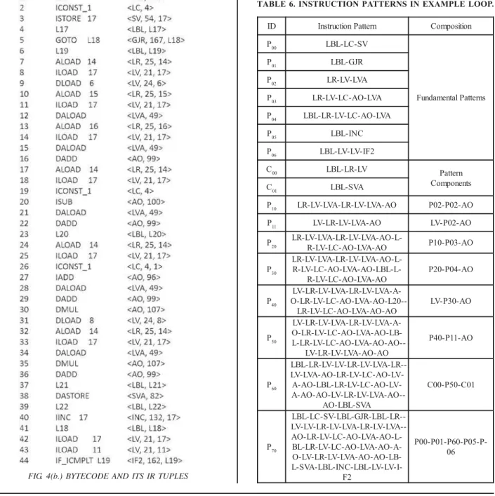
FIG. 4(b.) BYTECODE AND ITS IR TUPLES
4.3.3 Inter-Iteration Data Dependence
DOALL loops could be identified by making sure that loop iterations either does not contain any instruction patterns corresponding to memory access or they access independent memory locations. We need to identify instruction patterns that are used to read/write local variables, arrays elements and class members (i.e. fields) of both primitive and user-defined types. If a loop does not contain any instruction
D
I InsrtucitonPattern Compoisiton P00 LBL-LC-SV
s n r e tt a P l a t n e m a d n u F P01 LBL-GJR
P02 LR-LV-LVA
P03 LR-LV-LC-AO-LVA P04 LBL-LR-LV-LC-AO-LVA
P05 LBL-INC P06 LBL-LV-LV-IF2
C00 LBL-LR-LV Pattern
st n e n o p m o C C01 LBL-SVA
P10 LR-LV-LVA-LR-LV-LVA-AO P02-P02-AO
P11 LV-LR-LV-LVA-AO LV-P02-AO
P20 LR-LRV--LLVV-AL-CL-RA-OLV-L-LVVAA-A-AOO-L- P10-P03-AO
P30
-L -O A -A V L -V L -R L -A V L -V L -R L -L -L B L -O A -A V L -O A -C L -V L -R O A -A V L -O A -C L -V L
-R P20-P04-AO
P40
-A -A V L -V L -R L -A V L -V L -R L -V L -0 2 L -O A -A V L -O A -C L -V L -R L -O O A -O A -A V L -O A -C L -V L -R
L LV-P30-AO
P50
-A -A V L -V L -R L -A V L -V L -R L -V L -B L -O A -A V L -O A -C L -V L -R L -O -O A -O A -A V L -O A -C L -V L -R L -L O A -O A -A V L -V L -R L -V L O A -1 1 P -0 4 P
P60
-R L -A V L -V L -R L -V L -V L -R L -L B L -V L -O A -C L -V L -R L -O A -A V L -V L -V L -O A -C L -V L -R L -L B L -O A -A -O A -A V L -V L -R L -V L -O A -O A -A A V S -L B L -O A 1 0 C -0 5 P -0 0 C
P70
-R L -L B L -R J G -L B L -V S -C L -L B L -A V L -V L -R L -A V L -V L -R L -V L -V L -L -O A -A V L -O A -C L -V L -R L -O A -A -O A -A V L -O A -C L -V L -R L -L B -B L -O A -O A -A V L -V L -R L -V L -O -I -V L -V L -L B L -C N I -L B L -A V S -L 2 F -P -5 0 P -0 6 P -1 0 P -0 0 P 6 0
pattern corresponding to inter-iteration data dependences, it is DOALL loop because of independent iterations. Let’s analyze the loop given in Fig. 4 to determine if it is DOALL or not. Source code and Bytecode of the loop (Fig. 4) reveals that the only variables involved are local because compiled code does not contain any bytecode instruction related to class members (Fig. 4(b)). Table 7 shows the types and compiler-assigned indices of variables used by bytecode instructions. For example, loop index j is indexed at 17 and could be determined from IINC instruction. In Table 6, we can see that only one write operation, represented by P60, is performed in each iteration. This pattern has sixth level composition and its first component C00 contains information about the variable involved. The IR tuples of C00 are <LBL, L19>, <LR, 25, 14>, <LV, 21, 17> at line 6-8. It shows that the variable is indexed at 14 which is “double[] Gi”. Hence, we are concerned about the read/write patterns of array elements. Write operation of Gi depends on three read operations of Gi, one of which is performed in the same iteration and is harmless. Other two reads in an iteration j are performed in immediately previous iteration j-1 and next
iteration j+1, which causes inter-iteration data dependences. The patterns of reading Gi[j-1] and Gi[j+1] are P03 at line 17-21 and P04 at line 23-28, respectively. Hence, the loop in Figure 6 is not DOALL so could not be parallelized without resolving dependences.
4.4
Threading Framework
A threading mechanism is required by JIT compiler to modify selected loops for parallelization execution. We designed a Java threading framework to be generated directly in bytecode according to the characteristics of
el b ai r a
V Name Type Index
l a c o L
J int 17
1 m
N int 11
i
G doubel][ 14
r u o f _ r e v o _ a g e m
o doubel 6
1 m i
G doubel][ 15
1 p i
G doubel][ 16
a g e m o _ s u n i m _ e n
o Doubel 8
TABLE 7. VARIABLES USED IN EXAMPLE LOOP
workload. We adapted the idea of source code level JAVAR framework [40]. Our framework consists of only two classes, Workerijk and Managerijk, that are dynamically generated for each candidate loop lijk. We used ASM [41] for generation of framework classes (in bytecode) as dynamic part of classes would not be available at compile time[41]. Workerijk encapsulates the entire implementation of parallel task whereas Managerijk is responsible for creation and orchestration of workers. Managerijk contains only one static method work(…) and each candidate loop lijk is replaced with just a single call to Managerijk.work(…). Fig. 6 shows the interaction of threading framework with Classi that contain loop lijkin its method mij. For a loop lijk, a single Managerijk manages life cycle of n Workerijk threads. Each Workerijk calls runijk() method that is defined in Classi. The loop lijk is replaced with a call to Managerijk. work(...). Classi makes jxk calls for k DOALL loops in j methods of this class. Fig. 6 shows a cyclic dependency that could be removed by declaring runijk() before generating Workerijk and providing its definition after the generation of Managerijk. Actual usage of framework is elaborated in Section 5 using the code in Fig. 8.
4.5
Motivational Example
To demonstrate the step-by-step working of proposed methodology, we identify and parallelize the most suitable loop of JGF Series benchmark [24]. This benchmark manipulates various transcendental and trigonometric functions to calculate Fourier coefficients of function f(x) = (x+1)x. About 10,000 coefficients are computed with an interval of 0.2. Methodology starts with profiling phase in which we found that the application calls 28 methods i.e. Nm = 28. By setting TPC = 90%, we found 2 potential hotspots. For a potential hotspot, top-ranking value of PC is either due to its high CC (Call Count) or due to having compute intensive loops indicated by f10, f11 , f37, f38 features. The reason is that PC is based on the self-time consumed by a method i.e. self-time consumption of its callee methods is excluded. Looking at Table 8, we come to know that CC value of both methods is significantly high but only TrapezoidIntegrate() method contains one single loop. Hence, high time consumption (i.e. 99.9% collectively) of these methods is due to high call count and not due to the loops in their own code. To determine the immediate caller methods, we have to look at the
Managerijk Workerijk
+ Work (...) 1
1
n n
1
Manages Threads Life Cycle
+ id: Integer + ncores: Integer
Calls Work() Call run ()ijk
1... jxk
Classi
...
...
...
...
hotspot (...)j
run (...)ijk
...
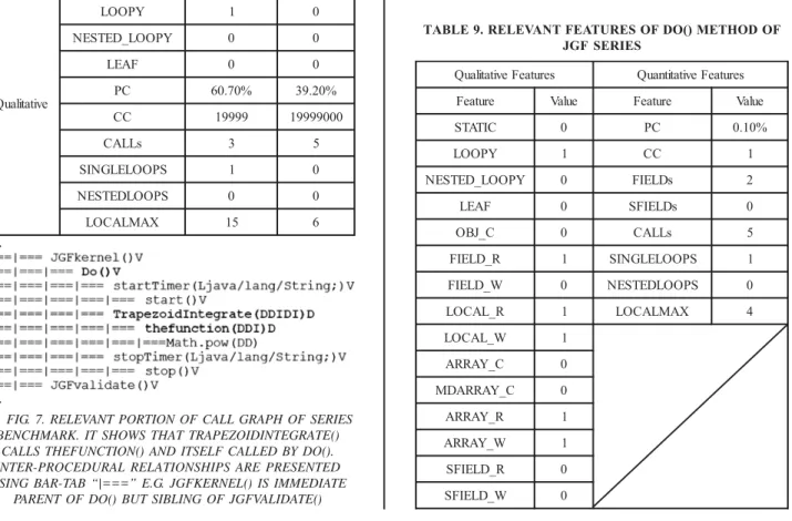
relevant portion of application call graph shown in Fig. 7. It shows that Do()method calls TrapezoidIntegrate() and TrapezoidIntegrate() calls thefunction(). In Table 9, qualitative features show that Do() method is (1) non-static (2) contains single loop(s) only (3) calls other methods (not leaf in call graph) (4) does not create any object and 1-D or n-D array (5) reads/writes array elements and local variables (6) only reads non-static class fields, and (7) does not read/write static class fields. Quantitative features say that Do() methodis (1) called only once (2) contains one single loop (3) reads two non-static class fields (4) has five call sites, and (5) reads/writes up to four local variables. Although self-time consumption of Do() method is 0.1%, it calls two most time consuming methods in a single loop and itself is called once. Hence, the loop in it is exploitable for parallelize execution.
5.
IMPLEMENTATION DETAILS
Implementation details include the steps taken to parallelize a candidate loop and a short note on proof of concept. All modifications are done on bytecode, as elaborated in section 4.
5.1
Parallelization Steps
Modifications steps are explained here in terms of Java source code. Bytecode level implementations details are given in section 5.2.
Loop Extraction: The loop is shown at line 7-10 of
Fig. 8(a) in source code of Do() method. Bytecode of this loop is extracted from the method and represented as IR tuples to recognize instruction patterns for data dependence analysis.
Data Dependence Analysis: Bytecode of Do() method
contains instruction patterns of local variable read/write. Besides loop index i, one local variable omega is defined e
p y
T Name TIrnatpegerzaotied FuTnhceiton
e v it a til a u Q C I T A T
S 0 0
Y P O O
L 1 0
Y P O O L _ D E T S E
N 0 0
F A E
L 0 0
C
P 60.70% 39.20%
C
C 19999 19999000 s
L L A
C 3 5
S P O O L E L G N I
S 1 0
S P O O L D E T S E
N 0 0
X A M L A C O
L 15 6
TABLE 8. FEATURES OF POTENTIAL HOTSPOTS IN JGF SERIES
FIG. 7. RELEVANT PORTION OF CALL GRAPH OF SERIES BENCHMARK. IT SHOWS THAT TRAPEZOIDINTEGRATE()
CALLS THEFUNCTION() AND ITSELF CALLED BY DO(). INTER-PROCEDURAL RELATIONSHIPS ARE PRESENTED USING BAR-TAB “|===” E.G. JGFKERNEL() IS IMMEDIATE
PARENT OF DO() BUT SIBLING OF JGFVALIDATE()
s e r u t a e F e v it a til a u
Q QuanttiaitveFeatures
e r u t a e
F Value Feature Value
C I T A T
S 0 PC 0.10%
Y P O O
L 1 CC 1
Y P O O L _ D E T S E
N 0 FIELDs 2
F A E
L 0 SFIELDs 0
C _ J B
O 0 CALLs 5
R _ D L E I
F 1 SINGLELOOPS 1
W _ D L E I
F 0 NESTEDLOOPS 0
R _ L A C O
L 1 LOCALMAX 4
W _ L A C O L 1 C _ Y A R R A 0 C _ Y A R R A D M 0 R _ Y A R R A 1 W _ Y A R R A 1 R _ D L E I F S 0 W _ D L E I F S 0
before the loop body and used in loop body. Local variables omega and i are not written in the loop body so there is no inter-iteration data dependence due to local variables. Table 9 shows that no static field is read/written and non-static fields are read but not written. However, arrays are read/written but source code does not show any array read. The bytecode reveals that in TestArray[][] write, TestArray[] is first loaded on stack and then its TestArray[][i] element is written. There is no data dependence due to TestArray[][i] because it is independently written in each iteration and without involving a read. Hence, the loop is DOALL and we can parallelize it.
Declaration of Run
ijk() Method: A method runijk is
declared in the class of Do() method, as shown in Fig. 8(b), where a, b, c are <start, end, step> tuple for a worker thread. We cannot define runijk yet because <start, end, step> is calculated in dynamically generated partitionLoop() method of Workerijk class. We just declare runijk here so that a call in Workerijk could not pop error.
Generation of Worker
ijk and Managerijk Classes: Next
step is to generate and load Workerijk and Managerijk classes. We observed that all classes have to be loaded by the same class loader as that of the application. Against the source code shown in Fig. 8(c-d), bytecode is generated using ASM[41].
Definition of Runijk() Method: Due to cyclic dependency
shown in Fig. 6, we define runijk() after code generation for Workerijk and Managerijk classes. Fig. 8(b) shows this definition, where calculation of a, b, c depends on the number of workers created in Mangerijk i.e. kept equal to number of CPU cores as shown in Fig. 8(d).
Loop Replacement in Hotspot: Finally, the loop in Do()
method is replaced with a single call to Managerijk.work() method as shown on line 7 of Fig. 8(e). Original loop and its replacement is encircled by dotted line to highlight in Fig. 8 (a) and Fig. 8(e), respectively.
5.2
Proof of Concept
As a proof of concept, we implemented a research prototype by extending SeekBin[22]. As a Java agent, it hooks JVM’s class loader, captures classes loading into JVM, and manipulates bytecode just before loading. SeekBin reads sorted flat profile F to determine the classes to be manipulated. Classes are parsed, transformed and generated (i.e. Managerijk, Workerijk) using ASM bytecode engineering library and loaded using java.lang.instrument API. The tool can profile and parse any sequential application to generate qualitative and quantitative features, IR tuples, instruction patterns, loop profiling, class generation and loading etc.
6.
CASE STUDIES
Data is collected by profiling and parsing eighteen benchmark applications [24] to analyze their parallelization potential. Data is analyzed for code comprehension regarding exploitable parallelism.
6.1
Code Comprehension
1 void Do() {
2 double omega;
3 JGFInstrumentor.startTimer(“Section2:Series:Kernel”);
4 TestArray[0][0] = TrapezoidIntegrate((double)0.0, (double)2.0, 1000,(double)0.0,0)/(double)2.0; 5 omega = (double) 3.1415926535897932;
6
7 for (inti = 1; i<array_rows; i++) {
8 TestArray[0][i] = TrapezoidIntegrate((double)0.0,(double)2.0,1000,omega * (double)i,1); 9 TestArray[1][i] = TrapezoidIntegrate((double)0.0,(double)2.0,1000,omega * (double)i,2);
10 }
11
12 JGFInstrumentor.stopTimer(“Section2:Series:Kernel”); 13 }
(a) SOURCE CODE OF DO() METHOD OF SERIES BENCHMARK
void runijk(int a, int b, int c, double omega){ for (inti = a; i< b; i = i+c) {
TestArray[0][i] = TrapezoidIntegrate((double)0.0,(double)2.0,1000,omega * (double)i,1); TestArray[1][i] = TrapezoidIntegrate((double)0.0,(double)2.0,1000,omega * (double)i,2); }
}
(b) DEFINITION OF RUNijk
public class Workerijk implements Runnable{
int ID, ncores, a, b, c, fr, to, step; SeriesTesttc;
double l1;
Workerijk(SeriesTest cls, int aa,
int bb, int cc, intnc, int id, double v1){ tc = cls; ID = id; ncores = nc;
a = aa; b = bb; c = cc; l1 = v1;
}
private void partitionLoop(){ step = c;
intblk = (b + ncores-1)/ncores; fr = ID*blk;
if(ID == 0) fr = ID*blk+1; to = (ID+1)*blk;
if (to > b ) to = b; } public void run() {
partitionLoop(); tc.runijk(fr,to,step, l1);
} }
public class Workerijk implements Runnable{
int ID, ncores, a, b, c, fr, to, step; SeriesTesttc;
double l1;
Workerijk(SeriesTest cls, int aa,
int bb, int cc, intnc, int id, double v1){ tc = cls; ID = id; ncores = nc;
a = aa; b = bb; c = cc; l1 = v1;
}
private void partitionLoop(){ step = c;
intblk = (b + ncores-1)/ncores; fr = ID*blk;
if(ID == 0) fr = ID*blk+1; to = (ID+1)*blk; if (to > b ) to = b; } public void run() {
partitionLoop(); tc.runijk(fr,to,step, l1);
} }
(c) DEFINITION OF WORKERijk CLASS (d) DEFINITION OF MANAGERijk CLASS
1 void Do() {
2 double omega;
3 JGFInstrumentor.startTimer(“Section2:Series:Kernel”);
4 TestArray[0][0]=TrapezoidIntegrate((double)0.0, (double)2.0, 1000,(double)0.0,0)/(double)2.0; 5 omega = (double) 3.1415926535897932;
6
7 Managerijk.work(this, 1, array_rows, 1, omega);
8
9 JGFInstrumentor.stopTimer(“Section2:Series:Kernel”); 10 }
6.2
Parallelization of JGF Benchmarks
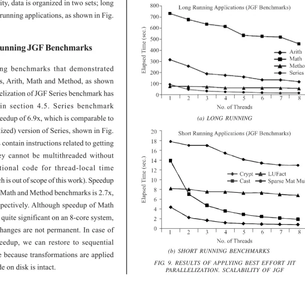
Thirteen benchmark applications are explicitly transformed and eight benchmarks showed a reasonable speedup, as shown in Fig. 9. Instead of exposing hidden parallelism in other benchmarks, proposed best effort approach prefers to restore sequential versions of applications that do not show speedup. To demonstrate the scalability of transformed applications, we passed “number of workers” as command line argument, instead of getting it from target system as mentioned in Fig. 8(d). Transformed applications are run on an 8-core system comprising 2 x Quad Core Intel® Xeon® E5405, 1333 MHz FSB, CPU Speed 2.0 GHz, L1 D Cache 32 KB, L1 I Cache 32 KB, L2 Cache 2x(2x6 ) = 24 MB and 8 GB DRAM. In order to assess the scalability, data is organized in two sets; long running and short running applications, as shown in Fig. 9(a-b).
6.2.1 Long Running JGF Benchmarks
Four long running benchmarks that demonstrated speedup are Series, Arith, Math and Method, as shown in Fig. 9(a). Parallelization of JGF Series benchmark has been described in section 4.5. Series benchmark demonstrated a speedup of 6.9x, which is comparable to HP (Hand Parallelized) version of Series, shown in Fig. 10(d). Outer loops contain instructions related to getting system time. They cannot be multithreaded without generating additional code for thread-local time management (which is out of scope of this work). Speedup observed in Arith, Math and Method benchmarks is 2.7x, 1.6x and 1.4x, respectively. Although speedup of Math and Method is not quite significant on an 8-core system, the point is that changes are not permanent. In case of unsatisfactory speedup, we can restore to sequential execution anytime because transformations are applied at runtime and code on disk is intact.
6.2.2 Short Running JGF Benchmarks
Short running benchmarks that showed speedup are Crypt, LUFact, SparseMatMult and Cast, as shown in Fig. 9(b). In Crypt, out of 30 methods, only one method cipher_idea() consumes 90% time when called twice in the application, as shown in Table 10. In cipher_idea(), there is no single loop and one 2-level nested loop. Nested loop is DOALL and its outer loop is parallelized.
Crypt demonstrated a speedup of 5.8x and perfectly scale with the increasing number of threads, as shown in Fig. 9(b). HP version of JGF Crypt, when run on the same system, demonstrated 7x speedup and resembling scalability, as shown in Fig. 10(c). The result is quite encouraging because proposed methodology is
(a) LONG RUNNING
(b) SHORT RUNNING BENCHMARKS
transforming code on-the-fly. In LUFact, only 4 out of 32 methods consume 90.8% time. LUFact contains 15 single and 4 nested loops. However, selected 4 methods contain 4 single and 1 nested loops (collectively), as shown in Table 10. Most time consuming method dgefa() is called once and contains one 2-level nested loop. Method daxpy() and idamax() are called in inner and outer loops of dgefa()’s nested loop, respectively. Outer loop is parallelized to achieve a speedup of 1.2x on 8-core system. On the same system, the speedup is not encouraging as compared to 4x speedup of HP JGF LUFact, as shown in Fig. 10(a). Looking at the code of HP version, we observed that this version achieved speedup by using barrier construct at four locations to synchronize the threads. This type of flexibility is not supported yet in our approach.
SparseMatMult calls 27 unique methods but only two methods consumed 90.1% time in a single call each, as shown in Table 10. Most time consuming method test() contains one single and one 2-level nested loop and second method JGFinitialise() contains one single loop. There is no harmful data dependences in all 3 loops, however, single loops contain trivial amount of computation. On parallelizing all 3 loops, we observed performance degradation as compared to sequential version. By parallelizing only nested loop of test(), we observed the scalability shown in Fig. 9(b), with a speedup of 1.4x. Running HP version on the same system, we observed a speedup of 4.1x. Scalability comparison of both versions is given in Fig. 10(b). HP version achieves this speed up by restructuring the implemented algorithm. For proper load balancing, signature of hotspot test() is
(a) LUFACT BENCHMARK (b) SPARSEMATMULT BENCHMARK
(c) CRYPT BENCHMARK (d) SERIES BENCHMARK. HP MIGHT OCCASIONALLY INVOLVE ALGORITHM RESTRUCTURING
changed to control the nested loop partitioning from outside the hotspot. Due to the reasons mentioned in section 1, proposed methodology works locally (i.e. within a hotspot only) without altering the interface (i.e. signature) of hotspot methods
Cast benchmark called 19 methods and by setting TPC = 90%, we converged to 6 methods that collectively consume 91.7% time of application (Table 10). Starting from most time consuming method JGFrun(), we found 4 nested loops here and this method is called once. Only a single loop is found in one of other 5 methods i.e., in printperf(). In nested loops, compute intensive code was found in inner loops that were parallelized. Outer loops contain timing routines and cannot be parallelized due to the reason mentioned in section 6.2.1. JGF Cast demonstrated
highest speedup of 7.6x. Overall, the observed speedup is in the range 1.2 - 7.6x.
7.
CONCLUSIONS
This work emphasizes that best effort JIT compiler inspired parallelization has great potential of parallelizing executable code at runtime. Loops in compute-intensive applications exhibit greater parallelization potential, which makes it a worthwhile option. Although it may not be able to parallelize each and every application, it is plausible to exploit parallelism without programmer intervention. Best effort exploits parallelism wherever possible and there is no harm because transformations are not made permanent. In case of failure, sequential execution could be restored. However, in case of success, transformations could be made permanent at any time. The main contributions of this paper include: (1) catalogs of qualitative and
k r a m h c n e
B TPC =100% TPC=90%
m
N f46 f37 f38 f39 f40 Nh f46 f37 f38 f39 f40
h ti r
A 19 1805 1 12 2843 1929 1 1 0 12 2249 1913
n g is s
A 21 1597 1 10 2802 1916 1 1 0 10 2114 1900
ts a
C 19 641 1 4 1458 776 6 146 1 4 1033 776
e t a e r
C 29 1E+08 1 15 3119 2155 2 2E+07 0 15 2455 2139
p o o
L 19 482 1 3 819 186 7 161 1 3 427 186
h t a
M 19 3875 1 30 5308 3904 1 1 0 30 4714 3888
d o h t e
M 33 9E+07 1 8 1749 927 7 6E+07 0 8 1106 911
l ai r e
S 25 2E+06 9 4 1738 708 1 1 8 4 1142 692
t p y r
C 30 48 8 1 1966 798 1 2 0 1 390 374
T F
F 30 37 5 2 1663 563 2 3 1 1 472 399
tr o S p a e
H 28 2E+06 4 1 1079 230 2 1E+06 2 1 156 131
t c a F U
L 32 3E+05 15 4 2169 820 4 3E+05 4 1 482 284
s ei r e
S 28 2E+07 2 1 1144 158 2 2E+07 1 0 115 22
R O
S 26 26 0 3 1058 147 2 2 0 3 218 147
tl u M t a M e s r a p
S 27 27 3 1 1080 124 2 2 2 1 187 107
n y D l o
M 35 4E+05 12 3 3196 1349 4 3E+05 1 1 878 591
r e c a r T y a
R 68 4E+08 4 2 3092 525 4 4E+08 1 0 260 61
h c r a e S B
A 39 7E+07 18 2 3241 782 5 5E+07 4 2 816 354
qualitative features for runtime code comprehension; (2) compact intermediate representation of ISA and instruction pattern recognition for dependence analysis; (3) threading framework; and (4) a set of algorithms to profile and parallelize DOALL loops.
With increasing number of cores per chip, it is now possible to use at least part of this compute power to analyze the runtime characteristics of an application with minimal impact on expected performance. Such information can be exploited to improve the application performance. Such approaches are particularly beneficial for complex long-running applications, which may not be simple to analyze manually. Loops are one of the simplest constructs that can be extracted from any type of code. Our work is an effort to demonstrate the feasibility of this approach. In past efforts, success criteria of an automated or semi-automated parallelization approach has been based on achievable speedup. When compared with manually parallelized applications, these approaches do not fare well because one parallelization technique may work for a few parts of the code but degrades others. Restricting to hotspots and ability to reverse parallelization transforms at runtime enhances the possibilities of parallelizing long running compute-intensive applications. By relaxing the speedup requirements, it is possible to try multiple techniques for different parts of application code at runtime to achieve optimal performance with no user input.
8.
FUTURE WORK
This work proposes a best effort parallelization methodology that could be used within the front end of JIT (i.e. dynamic) compiler. Integration of this methodology in an actual dynamic compiler is the obvious next step. We have designed a development project to integrate this methodology in an open source JIT compiler.
ACKNOWLEDGEMENT
This research was conducted during Ph.D. study of first author, at University of Engineering & Technology, Lahore, Pakistan.
REFERENCES
[1] Zhang, T.Y., and Suen, C.Y., “A Fast Parallel Algorithm for Thinning Digital Patterns”, Communications of the ACM, Volume 27, No. 3, pp. 236-239, 1984. [2] Alfredo Buttaria, J.L., Kurzaka, J., and Dongarra, J., “A
Class of Parallel Tiled Linear Algebra Algorithms for Multicore Architectures”, Parallel Computing Volume 35, No. 1, pp. 38-53, 2009.
[3] Wang, Y., Fan, J., Liu, W., and Han, Y., “A Parallel Algorithm to Construct BISTs on Parity Cubes”, IEE Proceedings of 2nd International Conference on Information Science and Control Engineering, pp. 54-58, 2015.
[4] Polychronopoulos, C.D., Girkar, M., Haghighat, M.R., Lee, C.L., Leung, B., and Schouten, D., “Parafrase-2: An Environment for Parallelizing, Partitioning, Synchronizing, and Scheduling Programs on Multiprocessors”, International Journal of High Speed Computing, Volume 1, No. 1, pp. 45-72, 1989. [5] Haghighat, M., and Polychronopoulos, C., “Symbolic
Program Analysis and Optimization for Parallelizing Compilers”, Springer Berlin Heidelberg, pp. 538-562, 1993.
[6] Whaley, J., and Kozyrakis, C., “Heuristics for Profile-Driven Method-Level Speculative Parallelization”, Proceedings of International Conference on Parallel Processing, pp. 147-156, 2005.
[7] Tournavitis, G., Wang, Z., Franke, B., and O’Boyle, M.F.P., “Towards a Holistic Approach to Auto-Parallelization: Integrating Profile-Driven Parallelism Detection and Machine-Learning Based Mapping”, ACM SIGPLAN Notices, Volume 44, No. 6, pp. 177-187, 2009.
[8] Jang, H., Kim, C., and Lee, J.W., “Practical Speculative Parallelization of Variable-Length Decompression Algorithms”, ACM SIGPLAN Notices, Volume 48, pp. 55-64, 2013.
[9] Jimborean, A., Clauss, P., Martinez, J.M., and Sukumaran-Rajam, A., “Online Dynamic Dependence Analysis for Speculative Polyhedral Parallelization”, Euro-Par, Parallel Processing, pp. 191-202, 2013.
[10] Liu, B., Zhao, Y., Li, Y., Sun, Y., and Feng, B., “A Thread Partitioning Approach for Speculative Multithreading”, The Journal of Supercomputing, Volume 67, No. 3, pp. 778-805, 2014.
[11] Yiapanis, P., Rosas-Ham, D., Brown, G., and Lujan, M., “Optimizing Software Runtime Systems for Speculative Parallelization”, ACM Transactions on Architecture and Code Optimization, Volume 9 No. 4, 2013.
[13] Aumage, O., Barthou, D., Haine, C., and Meunier, T., “Detecting Simdization Opportunities through Static/ Dynamic Dependence Analysis”, Euro-Par: Parallel Processing Workshops, Lecture Notes in Computer Science, Volume 8374, pp. 637-646, 2014.
[14] Tzenakis, G., Papatriantafyllou, A., Vandierendonck, H., Pratikakis, P., and Nikolopoulos, D., “BDDT: Block-Level Dynamic Dependence Analysis for Task-Based Parallelism”, Advanced Parallel Processing Technologies, Lecture Notes in Computer Science, Volume 8299, pp. 17-31, 2013.
[15] Verdoolaege, S., Carlos Juega, J., and Cohen, A., “Polyhedral Parallel Code Generation for CUDA”, ACM Transactions on Architure Code Optimum, Volume 9 No. 4, pp. 54:1-54:23, 2013.
[16] Steffan, J.G., Colohan, C.B., Zhai, A., and Mowry, T.C., “A Scalable Approach to Thread-Level Speculation”, ACM, Volume 28, No. 2, pp. 1-12, 2000.
[17] Harris, T., Cristal, A., Unsal, O.S., Ayguade, E., Gagliardi, F., Smith, B., and Valero, M., “Transactional Memory: An Overview”, IEEE Micro, Volume 27, No. 3, pp. 8-29, 2007.
[18] Bik, A.J., and Gannon, D., “A Prototype Bytecode Parallelization Tool”, Concurrency - Practice and Experience, Volume 10, Nos.11-13, pp. 879-885, 1998. [19] Aycock, J., “A Brief History of Just-in-Time”, ACM Computing Surveys, Volume 35, No. 2, pp. 97-113, 2003.
[20] Pemberton, S., and Daniels, M., “Pascal Implementation: The P4 Compiler and Interpreter”, Ellis Horwood, 1982. [21] Ierusalimschy, R., DeFigueiredo, L.H., and Celes, W., “The Implementation of Lua 5.0”, Journal of Universal Computer Science, Volume 11, No. 7, pp. 1159-1176, 2005.
[22] Mustafa, G., Waheed, A., and Mahmood, W., “SeekBin: An Automated Tool for Analyzing Thread Level Speculative Parallelization Potential”, Proceedings of 7th IEEE International Conference on Emerging Technologies, pp. 1-6, 2011.
[23] Knuth, D.E., “An Empirical Study of FORTRAN Programs”, Software: Practice and Experience, Volume 1, No. 2, pp. 105-133, 1971.
[24] Mathew, J. A., Coddington, P. D., and Ha-wick, K. A., “Analysis and development of Java Grande benchmarks,” Proc. 1999 conference on Java Grande, USA, ACM, pp. 72-80, 1999.
[25] Hinsen, K., “A Glimpse of the Future of Scientific Programming”, Computing in Science & Engineering, Volume 15, No. 1, pp. 84-88, 2013.
[26] Österlund, E., “Garbage Collection Supporting Automatic JIT Parallelization in JVM”, LNU, 2012.
[27] Österlund, E., and Löwe, W., “Analysis of Pure Methods Using Garbage Collection”, Proceedings of ACM SIGPLAN Workshop on Memory Systems Performance and Correctness, pp. 48-57, Beijing, China, 2012.
[28] Österlund, E., “Automatic Memory Management System for Automatic Parallelization”, LNU, 2011.
[29] Koch, T.J.K.E.V., and Björn, F., “Limits of Region-Based Dynamic Binary Parallelization”, SIGPLAN Notices, Volume 48, No. 7, pp. 13-22, 2013.
[30] Leung, A., Lhotak, O., and Lashari, G., “Automatic Parallelization for Graphics Processing units”, Proceedings of 7th International Conference on Principles and Practice of Programming in Java, Calgary, pp. 91-100, Alberta, Canada, 2009.
[31] Monteyne, M., “Rapidmind Multi-Core Development Platform”, RapidMind Inc., Waterloo, Canada, February, 2008.
[32] Hammacher, C., Streit, K., Hack, S., and Zeller, A., “Profiling Java Programs for Parallelism”, Proceedings of ICSE Workshop on Multicore Software Engineering, pp. 49-55, 2009.
[33] Christopher, J.F.P., Clark, V., and Allan, K., “LIBSPMT: A Library for Speculative Multithreading”, Sable Technical Report, 2007.
[34] Pickett, C.J.F., and Verbrugge, C., “SableSpMT: A Software Framework for Analysing Speculative Multithreading in Java”, Proceedings 6th ACM SIGPLAN-SIGSOFT Workshop on Program Analysis for Software Tools and Engineering, pp. 59-66, Portugal, 2005. [35] Carlstrom, B.D., Chung, J., Chafi, H., McDonald, A.,
Minh, C.C., Hammond, L., Kozyrakis, C., and Olukotun, K., “Transactional Execution of Java Programs”, OOPSLA Workshop on Synchronization and Concurrency in Object-Oriented Languages, 2005. [36] Chen, M.K., and Olukotun, K., “The JRPM System for
Dynamically Parallelizing Sequential Java Programs”, IEEE Micro, Volume 23, No. 6, pp. 26-35, 2003. [37] Kulkarni, M., Pingali, K., Walter, B., Ramanarayanan,
G., Bala, K., and Chew, L.P., “Optimistic Parallelism Requires Abstractions”, Communication ACM, Volume 52, No. 9, pp. 89-97, 2009.
[38] Chan, B., and Abdelrahman, T.S., “Run-Time Support for the Automatic Parallelization of Java Programs”, Journal Supercomputer, Volume 28, No. 1, pp. 91-117, 2004.
[39] Singer, J., Brown, G., Luján, M., Pocock, A., and Yiapanis, P., “Fundamental Nano-Patterns to Characterize and Classify Java Methods”, Electronic Notes in Theoretical Computer Science, Volume 253, No. 7, pp. 191-204, 2010.
[40] Bik A. J. C., and Gannon D. B., “Automatically exploiting implicit parallelism in Java,” Concurrency: Practice and Experience, vol. 9, no. 6, pp. 579–619, 1997. [41] Bruneton, E., Lenglet, R., and Coupaye, T., “ASM: A