Minimum Field Strength Simulator for Proton
Density Weighted MRI
Ziyue Wu1,2*, Weiyi Chen1, Krishna S. Nayak1
1Ming Hsieh Department of Electrical Engineering, University of Southern California, Los Angeles, California, United States of America,2Department of Biomedical Engineering, University of Southern California, Los Angeles, California, United States of America
Abstract
Objective
To develop and evaluate a framework for simulating low-field proton-density weighted MRI acquisitions based on high-field acquisitions, which could be used to predict the minimum B0field strength requirements for MRI techniques. This framework would be particularly useful in the evaluation of de-noising and constrained reconstruction techniques.
Materials and Methods
Given MRI raw data, lower field MRI acquisitions can be simulated based on the signal and noise scaling with field strength. Certain assumptions are imposed for the simulation and their validity is discussed. A validation experiment was performed using a standard resolu-tion phantom imaged at 0.35 T, 1.5 T, 3 T, and 7 T. This framework was then applied to two sample proton-density weighted MRI applications that demonstrated estimation of minimum field strength requirements: real-time upper airway imaging and liver proton-density fat frac-tion measurement.
Results
The phantom experiment showed good agreement between simulated and measured images. The SNR difference between simulated and measured was8% for the 1.5T, 3T, and 7T cases which utilized scanners with the same geometry and from the same vendor. The measured SNR at 0.35T was 1.8- to 2.5-fold less than predicted likely due to unac-counted differences in the RF receive chain. The predicted minimum field strength require-ments for the two sample applications were 0.2 T and 0.3 T, respectively.
Conclusions
Under certain assumptions, low-field MRI acquisitions can be simulated from high-field MRI data. This enables prediction of the minimum field strength requirements for a broad range of MRI techniques.
a11111
OPEN ACCESS
Citation:Wu Z, Chen W, Nayak KS (2016) Minimum Field Strength Simulator for Proton Density Weighted MRI. PLoS ONE 11(5): e0154711. doi:10.1371/ journal.pone.0154711
Editor:Mara Cercignani, Brighton and Sussex Medical School, UNITED KINGDOM
Received:July 29, 2015
Accepted:April 18, 2016
Published:May 2, 2016
Copyright:© 2016 Wu et al. This is an open access article distributed under the terms of theCreative Commons Attribution License, which permits unrestricted use, distribution, and reproduction in any medium, provided the original author and source are credited.
Data Availability Statement:All relevant data are within the paper and its Supporting Information files.
Funding:This study was supported by the National Institutes of Health grant R01-HL105210 (http://www. nih.gov). The funders had no role in study design, data collection and analysis, decision to publish, or preparation of the manuscript.
Introduction
Magnetic resonance imaging (MRI) is one of the most powerful imaging modalities, and has had a significant impact on healthcare [1]. MRI is safe, non-invasive, non-ionizing, and is capa-ble of resolving tissues in three dimensions while providing several different types of tissue con-trast in a single examination. MRI has two notable limitations, cost and speed. These are highly relevant in an era where rising healthcare costs [2] have placed greater pressure on determining and optimizing the cost-effectiveness of imaging for specific clinical questions. To date, stan-dard clinical MRI (1.5 T/3 T) has proven to be cost-prohibitive for many potential screening and preventative medicine applications. Even for diagnostic applications, achieving better image quality without improving outcomes, at the expense of reducing access due to high cost, can be only counterproductive [3]. On the other hand, low-field MRI (0.5 T) can be much less expensive while still maintaining equivalent diagnostic values for certain applications, as demonstrated by Rutt et al. [4].
Several technological developments have helped to address the speed and temporal resolu-tion of MRI scanning. Fast gradients and parallel imaging have had a significant impact and are now available on almost all commercial MRI scanners. Constrained reconstruction [5], compressed sensing [6], and MR fingerprinting [7] are emerging techniques that provide the potential added benefit of de-noising. These technological advances are typically developed and tested first on high-field scanners, defined here as1.5 T.
The purpose of this work is to provide a framework for determining the minimum field strength requirements of novel MRI methods. Due to the difficulties in differentiating different species in k-space, the current framework is most appropriate for proton-density weighted (PDw) acquisitions. Using this tool, researchers could determine the relevance and applicabil-ity of their techniques at lower field strengths (e.g. 0.1 to 0.5 T) even if they have only had the opportunities to test them at high field strengths (e.g.1.5 T). When applied to de-noising techniques and constrained reconstruction, this could also enable researchers to determine if their techniques could enable a reduction in the cost of MRI, should such instruments be designed for their applications. In this manuscript, we provide phantom validation of this framework, and provide two illustrative examples of how to predict minimum field strength requirements.
The first example application is real-time upper airway imaging, for the assessment of sleep-disordered breathing. The lack of anatomical information is a major limitation for current sleep studies, and dynamic MRI has been shown [8–11] to be an promising method to fulfill this unmet need. The high cost associated with conventional clinical MRI scans is arguably the number one reason that prevents these methods from being applied to routine sleep studies. If the scans can be performed on low-field scanners at much lower cost, the option of including MRI in sleep studies will be much more realistic. Besides lower cost, reduced Lorentz force experienced by the gradient coils and hence lower acoustic noise is another attractive feature of low-field MRI, especially for imaging during sleep.
Materials and Methods
Modeling Assumptions
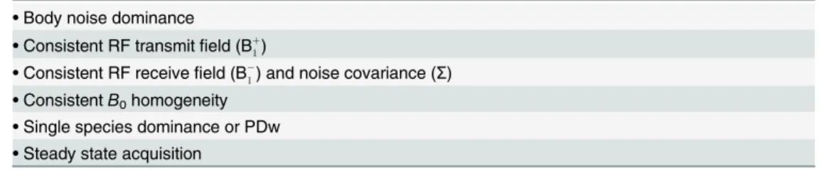
To simulate low-field acquisition from data acquired at high field strength, we make six assumptions, listed inTable 1, and explained below.
(1) Body noise dominance. We assume that body thermal noise is the dominant noise source at all field strengths under investigation (0.1–3.0 T). The validity of this assumption depends on field strength, imaging volume and the receiver coil. It has been shown that body noise dominance can be achieved at frequencies as low as 4 MHz in system sizes compatible with human extremity [15,16], suggesting the feasibility of performing most human scans with body noise dominance at 0.1 T or above.
(2) Consistent Bþ
1 field
We assume that the uniformity of RF transmission is consistent across field strengths. Since the RF operating frequencies go down at low field, the flip angle variation is expected to be smaller in real low-field imaging compared to our simulation.
(3) Consistent B1 field
We assume that the receiver coils have the same geometry and noise covariance at different field strengths. In order to simulate arbitrary B1 field, it would require accurate coil maps and noise covariance at both acquired and simulatedfields, which one may not have.
(4) Consistent B0homogeneity. We assume the same off-resonance in parts-per-million (ppm) at different field strengths. This results in less off-resonance in Hz at lower field.
(5) Single species dominance or PDw. We use a single global relaxation correction func-tion to account for the signal change at different field strengths. Because it is difficult to sepa-rate different species from k-space data, this assumption requires similar relaxation patterns at different field strengths for anything that contributes a significant portion to the signal in the region of interest. Although it may be unrealistic for some applications, this restriction can be relaxed in certain cases. For PDw imaging, the simulation is still valid when multiple major species are present (seeAppendixfor details).
(6) Steady state acquisition. If the signals are not acquired at steady state, the magnetiza-tion relaxamagnetiza-tion will be determined not only by the sequence parameters but also by the initial state. As a result, a single global relaxation correction cannot be applied and a more complicate time-depend function would need to be calculated.
Simulation of Low Field Acquisition
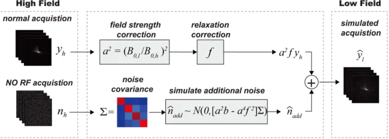
The process for simulating low-field data from high-field acquired data is illustrated inFig 1, and described here. The acquired high-field k-space data can be written as:
yh ¼ shþnh ð1Þ
Whereshandnhare pure signal and noise respectively. Under body noise dominance, both the Table 1. Assumptions for Low Field Acquisition.
•Body noise dominance •Consistent RF transmitfield (Bþ
1)
•Consistent RF receivefield (B1) and noise covariance (Σ) •ConsistentB0homogeneity
•Single species dominance or PDw •Steady state acquisition
real and imaginary parts of the k-space noisenhcan be modeled as multivariate normal distri-butions:
Refnhg Nð0;SÞ; Imfnhg Nð0;SÞ ð2Þ
WhereS2Rk×kis the noise covariance matrix for a k-channel receiver coil and is easily mea-sured by data acquisition with RF turned off. Since the thermal noise variance is proportional to B02and readout bandwidth BW, the simulated noisen^
lat lowfield becomes:
Ref^n
lg Nð0;a
2
bSÞ; Imfn^
lg Nð0;a
2
bSÞ; a¼B0;l
B0;h
; b¼BWl
BWh
ð3Þ
wherelandhstand for low and highfield respectively. The pure k-space signal at lowfield can be modeled as:
^s
l ¼ a
2
fsh ð4Þ
Wherefis a function that represents the signal change due to different relaxation behaviors at differentfields. This can be determined with knowledge of the sequence parameters and the dominant species’relaxation times. The details of calculatingffor common sequences are pro-vided in the Appendix. Givenf, the simulated lowfield k-space data can be written as:
^
yl ¼ ^slþn^l ¼ a
2
fshþn^l ð5Þ
we can rewrite it as:
^
yl¼a
2
fyhþ^nadd ð6Þ
Where^n
l ¼^naddþa
2
fnh, and from Eqs(2)&(3), we have
Refn^
addg Nð0;ða
2
b a4
f2
ÞSÞ; Imf^n
addg Nð0;ða
2
b a4
f2
ÞSÞ ð7Þ
Fig 1. Simulation of Low-field k-Space Data.High-field k-space datayhand pure noisenhare first acquired and served as input.yhis then scaled bya2
andfto account for signal magnitude change and different relaxation behaviors at different field strengths.fcan be determined based on steady state signal equations for different types of sequences (seeAppendixfor details). To simulate low-field datay^^
l;additional noise
^
n^
add, as calculated in the text, is
added to compensate for the different noise levels.
A MATLAB implementation based on the process above as well the examples in this article are available athttp://mrel.usc.edu/share.html.
Phantom Validation
To validate the proposed framework, a standard resolution phantom was scanned using a product sequence on 1.5T, 3T, and 7T whole body scanners, all from the same manufacturer (General Electric, Waukesha, WI). The phantom contains NiCl2H2O and H2O. T/R birdcage head coils (30cm diameter) were used at all field strengths. The 1.5T and 3T coils were single-channel. The 7T coil has two receive channels with nearly identical sensitivities; data from only one channel was used. We also scanned the same phantom on a 0.35T ViewRay scanner with a 12-channel torso coil. A single image was formed from all channels using sum of square. The scanner has a cylindrical bore similar to the 1.5T/3T/7T scanners, but is manu-factured by a different vendor. Due to its primary function as a MRI-guided radiation therapy instrument, the 0.35T scanner has a unique RF coil design to minimally obstruct the radia-tion source.
Identical acquisition parameters were used on all four scanners: 2D FSPGR with 62.5% par-tial k-space acquisition; FA 10°; TE/TR 3.1/10 ms; BW 31.25 KHz; FOV 25.6 cm; matrix size 256x160; slice thickness 5 mm. T1 and T2 values were measured using inversion recovery SE and SE sequence respectively. Homodyne reconstruction [17] was performed for all images. SNRs were measured in all cases on the magnitude images. For simulated images, the mean and standard deviation of SNR of twenty different simulations were calculated.
Real-time Upper Airway Imaging
For sleep apnea patients, airway compliance is measure of muscle collapsibility. This involves ultrafast 2D axial imaging of the airway and simultaneous airway pressure measurement [9]. During the process, negative pressure is generated by briefly blocking inspiration for one to three breaths. Under these circumstances, airway motion is extremely rapid, requiring about 10 frames per second and millimeter resolution. A custom sequence using 2D golden-angle radial FLASH [18] was implemented on the 3T scanner to acquire an oropharyngeal axial slice of one sleep apnea patient with a 6-channel carotid coil. Imaging parameters: 5° flip angle, 6 mm slice thickness, 1 mm2resolution, TE/TR 2.6/4.6 ms, BW 62.5 KHz. A separate scan with RF turned off was performed to calculate the noise covariance. Acquisitions at various low field strengths were simulated using the same imaging parameters.
Twenty-one spokes were used to reconstruct each temporal frame. Conventional gridding [19] was performed on the acquired 3T data and all simulated low-field data. CG-SENSE [20] was also performed with a temporal finite difference sparsity constraint [21]. The NUFFT tool-box [22] was used during algorithm implementation.
Fat-Water Separation
All studies involved were approved by the Institutional Review Board of Children's Hospital at Los Angeles and University of Southern California. Written informed consents were obtained from the participants.
Results
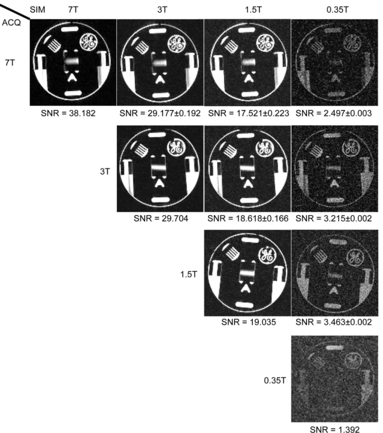
Phantom validation
Fig 2compares the image acquired and/or simulated at 0.35T, 1.5 T, 3 T, 7 T. The difference between simulated and measured mean SNR was less than 8% for all images at 1.5 T and 3 T respectively, which was considered to be good agreement. There were a 1.8–2.5 times of SNR differences for simulated and acquired images at 0.35T.
Real-time Upper Airway Imaging
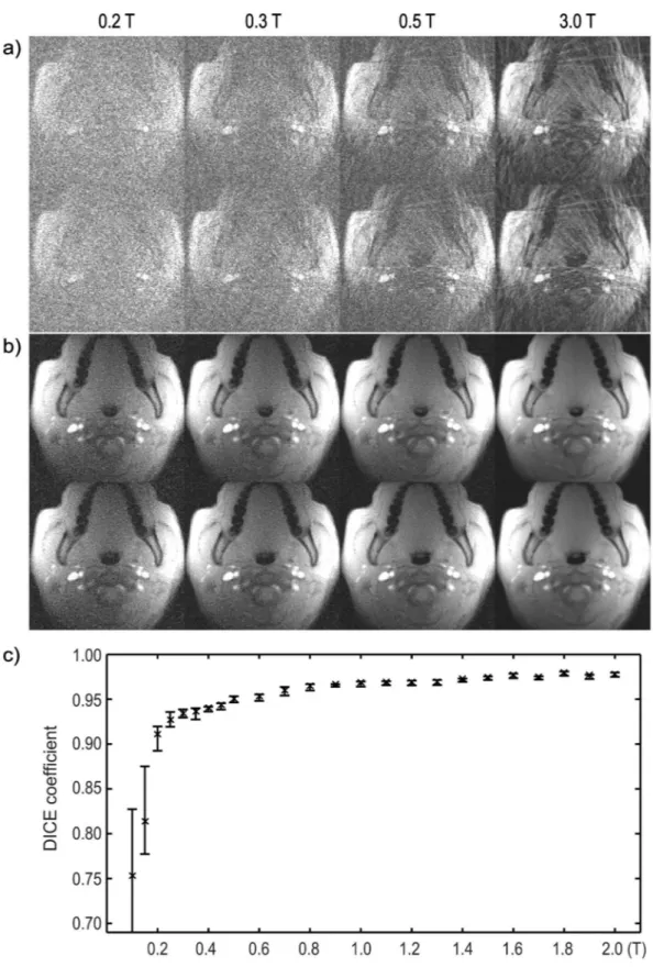
Fig 3shows two representative frames reconstructed at different field strengths, one with the airway partially collapsed (top rows in both a and b), and one with it open (bottom rows).Fig 3a and 3bcorrespond to gridding and CG-SENSE with temporal finite difference constraint, respectively. All reconstructed frames are also shown in theS1 Movie. The SNR becomes worse as field strength goes down, and the airway becomes completely unidentifiable below 0.3 T. With more advanced reconstructions in b, the noise and artifacts are reduced significantly. We then performed airway segmentation on these images based on a simple region-growing algo-rithm and show, inFig 3c, the average DICE coefficients over 100 temporal frames (3 breaths) at different field strengths. Segmented airways from the 3T images were used as the references. Fifty independent simulations were performed at each simulated field strength. Error bars cor-respond to 95% confidence intervals. In our experience, DICE coefficient>0.9 is acceptable for this application, suggesting that the minimum field requirement is 0.2 T. Note also that the DICE coefficients exhibit a sharp drop at 0.2 T and the variance increases significantly, imply-ing segmentation failures.
Fat-Water Separation
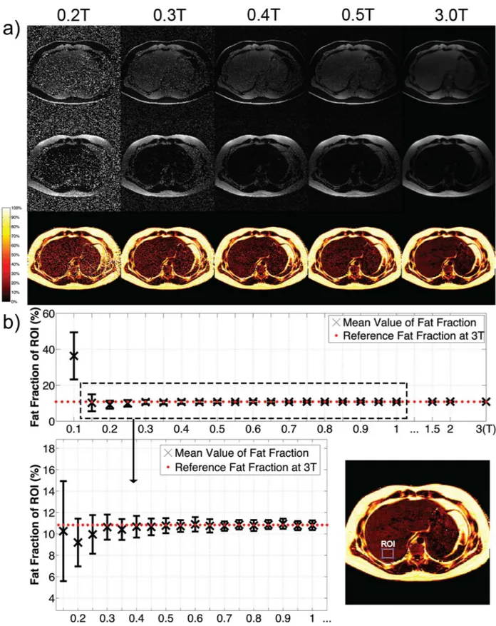
Fig 4acompares water-only, fat-only, and proton-density fat fraction images for a single axial slice at different field strengths. A region of interest (ROI) in the liver was manually selected andFig 4bshows the mean and standard deviation of the fat fraction inside the ROI, calculated from fifty independent simulations at each field strength. The precision (standard deviation) becomes worse as B0decreases. The accuracy (mean) deviates significantly at 0.1 T, a result of dominant noise making proton-density fat fraction biased towards 50%. Although the accuracy and precision needed for a clinical liver fat biomarker is not yet known [12], once determined, this type of analysis could facilitate determination of the required minimum field strength. For example, if the accuracy and precision needed are both 2%, then this analysis suggests a mini-mum field strength of 0.3 T would be sufficient.
Discussion
Fig 2. Phantom Validations of Simulated SNR Change.The acquired 0.35T/1.5T/3T/7T images and simulated images from data acquired at 3T and 7T respectively are listed for comparison. Measured SNR values are shown below each image. For simulated images, the mean and standard deviation of SNR of twenty different simulations were used. Contrast was adjusted for better noise visualization.
manufacturer with similar geometry and RF coils. To reduce the effects of B1 inhomogeneity and off-resonance, which are particularly severe at 7T, we used a small flip angle (10°) and short TE (3.1 ms) relative to T2 (100 ms) so that the validation can mostly reflect the accuracy of the assumptions and methods in this work. The phantom validation results exhibit a good match between the simulations and measurements on these scanners. It demonstrates that the assumptions we made are reasonable and the simulations based on them can give reliable pre-dictions. We also performed a phantom experiment on a 0.35T scanner with different geome-try and from a different vendor, with additional constraints on the RF receiver coil. The 1.8- to 2.5-fold SNR discrepancy between measurement and simulation at 0.35 T may be explained by unaccounted differences in the receive coils. The 0.35T ViewRay system is designed primarily for MRI-guided radiation therapy, therefore receiver coils are designed to minimally obstruct the desired radiation.
The proposed simulation framework has several limitations. First, because it is difficult to differentiate species with different relaxation properties in k-space, the framework only deals with PDw images, which significantly limits the number of real world applications. Second, some phenomena that were assumed to be independent of field strength, do actually change with field strength. For example, B0and B1uniformity are significantly improved at low-field, but the spatial distribution and the amount of the improvement is object specific. Phenomenon like physiological noise, must be experimentally studied and are extremely applications spe-cific. In our experience, these factors would be nearly impossible to incorporate into a general-purpose simulator. Therefore, what we chose is to make simplifying assumptions that represent a worst-case scenario in most cases. For example, we assume the same B1 homogeneity at low-field even though the B1 transmit and receive low-field will have equal or better homogeneity at low-field. Third, image quality at low field can be optimized by adjusting pulse sequence parameters (e.g. using higher flip angles, longer readouts and TR’s with a larger readout duty-cycle). This was not accounted for, as we assumed pulse sequence parameters were unchanged. This again represents a worst-case scenario. Fourth, we performed a rather narrow validation experiment with just one resolution phantom. This was purely for practical reasons; it was the only common phantom available at all sites. Future experiments would benefit from a phantom that included samples with different PD and relaxation parameters (e.g. a T1/T2 grid phantom) and potentially in vivo data collection, using multiple sequences at each field strength.
Many new MR imaging and reconstruction methods are developed at centers that utilize state-of-the-art high-field instruments. In addition to advancing performance at high field strengths, it is informative to determine the potential to apply these same techniques on more affordable low-field systems. New methods, if translated and implemented on low-field scan-ners, could enable many applications that are now prohibitive at low field because of insuffi-cient SNR. It is our experience that most MRI researchers today only have access to 1.5T/3T instruments, because they are the most widely used in the clinic. There are often significant logistical barriers to test ideas at low field. Getting an MR scanner, even a low field one, is a sig-nificant investment and the proposed simulation framework can provide a first-order approxi-mation of performance and feasibility, at no cost.
Low-field MRI has the potential to be more cost-efficient, and has many other attractive properties including reduced acoustic noise and specific absorption rate (SAR), safer for sub-jects with implants containing ferromagnetic components, more uniform RF transmission, and less off-resonance for the same part-per-million B0homogeneity. Lower RF frequencies also
over 100 temporal frames (3 breaths) at different field strengths. 3T images are served as references. Fifty independent simulations were performed at each field strength. Error bars correspond to 95% confidence intervals.
Fig 4. Application to Abdominal Fat-Water Separated Imaging.a) Fat-water separated images reconstructed from data acquired at 3 T and simulated at low fields. Top row: water only; middle: fat only; bottom: proton-density fat fractions. b) The mean and standard deviation of fat fraction in the ROI at different field strengths. Fifty independent simulations were performed at each field strength.
lead to decreased tissue conductivity and therefore higher RF transmission and reception effi-ciency, as quantitatively measured in [25,26]. If the effective SNR can be improved to reason-able levels with the help of better RF coil design, advanced imaging and reconstruction techniques, these nice features could further broaden the role of low-field MRI.
It is relatively straightforward to determine the minimum field strength requirement for new MRI methods under certain circumstances, as listed inTable 1. We have demonstrated the process, using modeling assumptions that are widely accepted in the MR community. How-ever, several precautions need to be taken before applying the model here. First, the model assumes the same sequence parameters at all field strengths. It would be natural to pick differ-ent parameters at low fields. Second, the model assumes the same scanner geometry and coil geometry. This is also not perfect, since many design constraints change at low fields and they all could impact the magnet and coil layout. Third, the receiver coil noise goes down more slowly than the body noise as field strength goes down [27]. The validity of body thermal noise dominance is questionable for ultra-low field (<0.1 T) and small volume imaging. Even in the range of 0.1 to 0.5 T, the requirement for suppressing receiver coil noise, although already achievable, is typically higher compared to at high fields. Finally, to achieve reasonable image quality at low fields, constrained reconstruction methods are likely to be involved in many applications. Although powerful, many of these methods have not been extensively validated yet. One needs to be extra careful with them, especially when the depiction of subtle features is important.
We would like to emphasize that due to the nature of MRI, poorer image quality is inevita-ble at low fields in almost all cases no matter what acquisition and reconstruction techniques are used. But as already been illustrated here and shown in several other low field studies [4,28–33], worse image quality doesnotnecessarily lead to less diagnostic value. With that in mind, selecting appropriate evaluation criteria becomes very important when comparing the results at different field strengths. If, for example, the sensitivity and specificity of the useful features are comparable at both high and low fields, then differences in root-mean-square error (RMSE) are likely to be inconsequential.
Appendix
Signal relaxation corrections for common sequences
Spin echo (SE/FSE/TSE). At steady state, the magnetization after excitation can be expressed as
Mss ¼ M0
1 E
1
1 E
1cosy
siny ðA1Þ
WhereM0is the longitudinal magnetization,θis theflip angle andE1=e−TR/T1. The acquired signal is
s¼Að1 E1Þsiny
1 E1cosy e
TE=T2
ðA2Þ
where A is a constant proportional toB2
function becomes
f ¼ ^sl
a2 sh
¼ ð1 E1;lÞsinyl
1 E
1;lcosyl
=ð1 E1;hÞsinyh
1 E
1;hcosyh
" #
e ðTEl TEhÞ=T2
ðA3Þ
landhstand for low and highfield respectively. For PDw imaging, where a) TE<<T2and b) TR>>T1or theflip angleθis low,fsinθl/sinθhregardless of the species type. As a result, the restriction of single species dominance can be relaxed and the equation above can be applied to multiple species types.
Gradient echo (GRE/FGRE/SPGR/FLASH). The signal change is similar to spin echo, except following T2decay:
f ¼ ^sl
a2 sh
¼ ð1 E1;lÞsinyl
1 E
1;lcosyl
=ð1 E1;hÞsinyh
1 E
1;hcosyh
" #
e ðTEl=T2
l TEh=T2hÞ ðA4Þ
In practice, one may not know the explicit values of T2, since it also depends on local B0 inho-mogeneity and susceptibility. Given [35]
1
T2¼ 1
T2þcgDBppmB0 ðA5Þ
where c is a constant andΔBppmis thefield inhomogeneity in parts-per-million. We can rewrite the exponential term in (A4) as:
e ðTEl=T2
l TEh=T2hÞ¼e ðTEl TEhÞ=T2e cgDBppmðB0;lTEl B0;hTEhÞ ðA6Þ
In cases where T2is difficult to estimate, T2may be used instead of T2. As long asB0,lTEl
B0,hTEh, this will lead to an underestimation of signal, which means the simulated SNR will be at best the same as the actual low-field acquisition.
In the airway example, T2is unknown, so T2is used instead. Given proton density weight-ing andθl=θh,f1. In the fat-water example, in order to generate the same fat-water phase
shift, the product of B0TE needs to remain the same, (A6) is reduced toe TEl TEhT2 . Since smallflip
anglesθl=θh= 3° were used,f e TEl TEhT2 , with liver T2set to 42 ms [27].
Balanced steady-state free precession (bSSFP, FIESTA, true FISP). The steady state transverse magnetization, assuming TE, TR<<T1, T2, is [36]:
Mss ¼ M0
siny
1þcosyþ ð1 cosyÞðT1=T2Þ ðA7Þ
based on similar calculations in a),fis now a function of T1, T2andflip angle:
f ¼ 1þcosyþ ð1 cosyÞðT1h=T2Þ
1þcosyþ ð1 cosyÞðT1
l=T2Þ
ðA8Þ
Inversion recovery (STIR, FLAIR). Following similar analysis, with 90° excitation, we have:
Mss ¼ M0ð1 2e
TI=T1
þE1Þ ðA9Þ
f ¼ ½ð1 2e TIl=T1;lþE
1;lÞ=ð1 2e
TIh=T1;hþE
1;hÞe
Since the inversion timeTIis usually chosen to null a particular species, the impact of this species on the signal can be neglected. Here T1is the value of the remaining dominant species.
Supporting Information
S1 Movie. Upper Airway Dynamics.The movie shows the whole 100 frames (3 breaths) reconstructed from simulated 0.2 T, 0.3 T, 0.5 T and acquired 3 T data (from left to right), as mentioned inFig 3. The region around the airway is zoomed in for better illustration purpose. Top row: gridding reconstruction; bottom row: CG-SENSE with temporal finite difference sparsity constraint.
(MP4)
Acknowledgments
We thank Steven Conolly and Angel Pineda for helpful discussions, Christoph Leuze and Jen-nifer McNab for help with 7T data acquisition, Shams Rashid and Peng Hu for help collecting 0.35T data, and Houchun Hu and Samir Sharma for assistance using the ISMRM fat-water toolbox.
Author Contributions
Conceived and designed the experiments: ZW KN. Performed the experiments: ZW WC. Ana-lyzed the data: ZW WC. Contributed reagents/materials/analysis tools: ZW WC. Wrote the paper: ZW WC KN.
References
1. Fuchs VR, Sox HC. Physicians’Views Of The Relative Importance Of Thirty Medical Innovations. Health Aff (Millwood). 2001; 20(5):30–42.
2. Iglehart JK. Health Insurers and Medical-Imaging Policy—A Work in Progress. N Engl J Med. 2009; 360(10):1030–7. doi:10.1056/NEJMhpr0808703PMID:19264694
3. Jhaveri K. Image quality versus outcomes. J Magn Reson Imaging. 2015; 41(4):866–9. doi:10.1002/ jmri.24622PMID:24677391
4. Rutt BK, Lee DH. The impact of field strength on image quality in MRI. J Magn Reson Imaging. 1996; 6 (1):57–62. PMID:8851404
5. Liang Z-P, Boda F, Constable R, Haacke EM, Lauterbur PC, Smith M. Constrained Reconstruction Methods in MR Imaging. Rev Magn Reson Med. 1992; 4:67–185.
6. Lustig M, Donoho DL, Santos JM, Pauly JM. Compressed Sensing MRI. IEEE Signal Process Mag. 2008;(2: ):72–82.
7. Ma D, Gulani V, Seiberlich N, Liu K, Sunshine JL, Duerk JL, et al. Magnetic resonance fingerprinting. Nature. 2013; 495(7440):187–92. doi:10.1038/nature11971PMID:23486058
8. Kim Y-C, Lebel RM, Wu Z, Ward SLD, Khoo MCK, Nayak KS. Real-time 3D magnetic resonance imag-ing of the pharyngeal airway in sleep apnea. Magn Reson Med. 2014; 71(4):1501–10. doi:10.1002/ mrm.24808PMID:23788203
9. Wu Z, Kim Y, Khoo MCK, Nayak KS. Novel upper airway compliance measurement using dynamic golden-angle radial FLASH. In: Proc ISMRM 22th Scientific Sessions. Milan, Italy; 2014. p. 4323.
10. Wagshul ME, Sin S, Lipton ML, Shifteh K, Arens R. Novel retrospective, respiratory-gating method enables 3D, high resolution, dynamic imaging of the upper airway during tidal breathing. Magn Reson Med. 2013; 70(6):1580–90. doi:10.1002/mrm.24608PMID:23401041
11. Shin LK, Holbrook AB, Capasso R, Kushida CA, Powell NB, Fischbein NJ, et al. Improved sleep MRI at 3 tesla in patients with obstructive sleep apnea. J Magn Reson Imaging. 2013; 38(5):1261–6. doi:10. 1002/jmri.24029PMID:23390078
13. Hu HH, Kan HE. Quantitative proton MR techniques for measuring fat. NMR Biomed. 2013; 26 (12):1609–29. doi:10.1002/nbm.3025PMID:24123229
14. Hu HH, Nayak KS, Goran MI. Assessment of abdominal adipose tissue and organ fat content by mag-netic resonance imaging. Obes Rev. 2011; 12(5):e504–15. doi:10.1111/j.1467-789X.2010.00824.x PMID:21348916
15. Chronik BA, Venook R, Conolly SM, Scott GC. Readout frequency requirements for dedicated prepolar-ized and hyperpolarprepolar-ized-gas MRI systems. In: Proceedings of the 10th Annual Meeting of ISMRM, Honolulu. Honolulu, HI, USA; 2002. p. 0058.
16. Grafendorfer T, Conolly S, Matter N, Pauly J, Scott G. Optimized Litz coil design for prepolarized extremity MRI. In: Proceedings of the 14th Annual Meeting of ISMRM, Seattle, WA, USA. Seattle, WA, USA; 2006. p. 2613.
17. Noll DC, Nishimura DG, Macovski A. Homodyne detection in magnetic resonance imaging. IEEE Trans Med Imaging. 1991; 10(2):154–63. PMID:18222812
18. Wu Z, Chen W, Khoo MCK, Davidson Ward SL, Nayak KS. Evaluation of upper airway collapsibility using real-time MRI. J Magn Reson Imaging. 2015. doi:10.1002/jmri.25133
19. Jackson JI, Meyer CH, Nishimura DG, Macovski A. Selection of a convolution function for Fourier inver-sion using gridding. IEEE Trans Med Imaging. 1991; 10(3):473–8. PMID:18222850
20. Pruessmann KP, Weiger M, Bornert P, Boesiger P. Advances in sensitivity encoding with arbitrary k-space trajectories. Magn Reson Med. 2001; 46(4):638–51. PMID:11590639
21. Feng L, Grimm R, Block KT, Chandarana H, Kim S, Xu J, et al. Golden-angle radial sparse parallel MRI: Combination of compressed sensing, parallel imaging, and golden-angle radial sampling for fast and flexible dynamic volumetric MRI. Magn Reson Med. 2014; 72(3):707–17. doi:10.1002/mrm.24980 PMID:24142845
22. Fessler JA, Sutton BP. Nonuniform fast Fourier transforms using min-max interpolation. Signal Process IEEE Trans On. 2003; 51(2):560–74.
23. Hernando D, Kellman P, Haldar JP, Liang Z-P. Robust water/fat separation in the presence of large field inhomogeneities using a graph cut algorithm. Magn Reson Med. 2010; 63(1):79–90. doi:10.1002/ mrm.22177PMID:19859956
24. Hu HH, Börnert P, Hernando D, Kellman P, Ma J, Reeder S, et al. ISMRM workshop on fat–water sepa-ration: Insights, applications and progress in MRI. Magn Reson Med. 2012; 68(2):378–88. doi:10. 1002/mrm.24369PMID:22693111
25. Winter L, Niendorf T. On the electrodynamic constraints and antenna array design for human in vivo MR up to 70 Tesla and EPR up to 3GHz. In: Proc Intl Soc Mag Reson Med. 2015.
26. Vaughan JT, Garwood M, Collins CM, Liu W, DelaBarre L, Adriany G, et al. 7T vs. 4T: RF power, homo-geneity, and signal-to-noise comparison in head images. Magn Reson Med. 2001; 46(1):24–30. PMID: 11443707
27. Nishimura DG. Principles of magnetic resonance imaging. Stanford University; 1996.
28. Ghazinoor S, Crues JV III. Low Field MRI: A Review of the Literature and Our Experience in Upper Extremity Imaging. Clin Sports Med. 2006; 25(3):591–606. PMID:16798144
29. Coffey AM, Truong ML, Chekmenev EY. Low-field MRI can be more sensitive than high-field MRI. J Magn Reson. 2013; 237:169–74. doi:10.1016/j.jmr.2013.10.013PMID:24239701
30. Pääkkö E, Reinikainen H, Lindholm E-L, Rissanen T. Low-field versus high-field MRI in diagnosing breast disorders. Eur Radiol. 2005; 15(7):1361–8. PMID:15711841
31. Merl T, Scholz M, Gerhardt P, Langer M, Laubenberger J, Weiss HD, et al. Results of a prospective multicenter study for evaluation of the diagnostic quality of an open whole-body low-field MRI unit. A comparison with high-field MRI measured by the applicable gold standard. Eur J Radiol. 1999; (1: ):43– 53.
32. Kersting-Sommerhoff B, Hof N, Lenz M, Gerhardt P. MRI of peripheral joints with a low-field dedicated system: A reliable and cost-effective alternative to high-field units? Eur Radiol. 1996; 6(4):561–5. PMID:8798043
33. Ejbjerg B, Narvestad E, Jacobsen S, Thomsen H, Ostergaard M. Optimised, low cost, low field dedi-cated extremity MRI is highly specific and sensitive for synovitis and bone erosions in rheumatoid arthri-tis wrist and finger joints: comparison with conventional high field MRI and radiography. Ann Rheum Dis. 2005; 64(9):1280–7. PMID:15650012
34. Bottomley PA, Hardy CJ, Argersinger RE, Allen‐Moore G. A review of 1H nuclear magnetic resonance relaxation in pathology: Are T1 and T2 diagnostic? Med Phys.1987; 14(1):1–37. PMID:3031439