www.atmos-chem-phys.net/12/10957/2012/ doi:10.5194/acp-12-10957-2012
© Author(s) 2012. CC Attribution 3.0 License.
Chemistry
and Physics
A fast SEVIRI simulator for quantifying retrieval uncertainties
in the CM SAF cloud physical property algorithm
B. J. Jonkheid1, R. A. Roebeling1,2, and E. van Meijgaard1
1Royal Netherlands Meteorological Institute (KNMI), De Bilt, The Netherlands
2European Organisation for the Exploitation of Meteorological Satellites (EUMETSAT), Darmstadt, Germany
Correspondence to:B. J. Jonkheid ([email protected])
Received: 26 August 2011 – Published in Atmos. Chem. Phys. Discuss.: 7 February 2012 Revised: 24 October 2012 – Accepted: 2 November 2012 – Published: 20 November 2012
Abstract.The uncertainties in the cloud physical properties derived from satellite observations make it difficult to inter-pret model evaluation studies. In this paper, the uncertainties in the cloud water path (CWP) retrievals derived with the cloud physical properties retrieval algorithm (CPP) of the climate monitoring satellite application facility (CM SAF) are investigated. To this end, a numerical simulator of MSG-SEVIRI observations has been developed that calculates the reflectances at 0.64 and 1.63 µm for a wide range of cloud parameter values, satellite viewing geometries and surface albedos using a plane-parallel radiative transfer model. The reflectances thus obtained are used as input to CPP, and the retrieved values of CWP are compared to the original input of the simulator. Cloud parameters considered in this paper refer to e.g. sub-pixel broken clouds and the simultaneous occurrence of ice and liquid water clouds within one pixel. These configurations are not represented in the CPP algo-rithm and as such the associated retrieval uncertainties are potentially substantial.
It is shown that the CWP retrievals are very sensitive to the assumptions made in the CPP code. The CWP retrieval errors are generally small for unbroken single-layer clouds with COT>10, with retrieval errors of∼3 % for liquid wa-ter clouds to∼10 % for ice clouds. In a multi-layer cloud, when both liquid water and ice clouds are present in a pixel, the CWP retrieval errors increase dramatically; depending on the cloud, this can lead to uncertainties of 40–80 %. CWP re-trievals also become more uncertain when the cloud does not cover the entire pixel, leading to errors of∼50 % for cloud fractions of 0.75 and even larger errors for smaller cloud frac-tions. Thus, the satellite retrieval of cloud physical properties of broken clouds as well as multi-layer clouds is complicated
by inherent difficulties, and the proper interpretation of such retrievals requires extra care.
1 Introduction
Clouds play a significant role in the climate system, since they influence the atmospheric energy balance by scattering and absorbing solar and terrestrial radiation, and by playing a key role in the atmospheric water cycle. Thus, it is important for climate models to treat clouds as accurately as possible. Comparison of model cloud physical properties with satellite observations is a valuable tool in providing accurate cloud statistics (Roebeling et al., 2006).
II
IV
model cloud field
observed radiances simulated radiances
retrieved cloud properties simulated cloud properties real cloud field
I III
satellite observations
retrieval retrieval algorithm algorithm
forward model
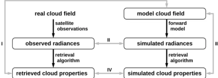
Fig. 1.Diagram of the comparison of climate model cloud fields with observations. The left side represents the observations of real clouds and the retrieval of satellite products, while the right side represents the model with simulated level 1 and level 2 satellite products. The boxes represent the available data sets, and the grey double-headed arrows represent routes along which comparisons can be performed between them. It should be noted that route III does not involve any reference to the real cloud field, but it is used to diagnose the climate model-forward model-retrieval chain.
between the input cloud parameters and the products is use-ful to diagnose the climate model-forward model-retrieval al-gorithm chain. In route IV, satellite products are simulated from the model output and compared to the observed prod-ucts. This route has the same advantages as route II; more-over, differences between model output and satellite data are easier to interpret.
The classical methodology in model evaluation is to com-pare model fields directly with retrieved and collocated satel-lite products (i.e. route I in Fig. 1). Examples using this methodology are Molders et al. (1995), who evaluated cloud cover parametrization schemes with NOAA9 AVHRR data; Tselioudis and Jakob (2002) evaluated seasonal cloud prop-erty distributions of mid-latitude clouds in weather and cli-mate models (ECMWF and GISS, respectively) with ISCCP observations; Roebeling and van Meijgaard (2009) evaluated diurnal variations in cloud physical properties by compar-ing statistics in model and satellite retrievals; and recently Greuell et al. (2011) evaluated a climate model using earth radiation budget observations from the GERB instrument and cloud physical properties from SEVIRI. The main disadvan-tage of such classical model evaluations is that model-to-satellite differences are partly due to model errors, partly due to inadequate satellite retrieval assumptions and finally due to intrinsic differences in the definitions of model and satel-lite products. Because of this entanglement of uncertainties in both the satellite retrievals and the model formulation of cloud parameters, it is difficult to assess model performance based on such an evaluation alone.
This paper aims to quantify the uncertainties in the cloud physical properties (CPP) retrieval algorithm of the climate monitoring satellite application facility (CM SAF), which uses the reflectances at 0.64 and 1.63 µm in the Nakajima and King (1990) method (see Fig. 2) to retrieve COT and
reff, from which CWP can be calculated. The goal is to de-termine the circumstances under which the cloud properties
Fig. 2.The Nakajima and King (1990) retrieval method. Each curve shows the values of reflectances at 0.64 and 1.63 µm for a certain value ofreffas a function of COT (indicated by the mostly vertical lines). Thus, from a combination of these reflectances both the COT and reff of a cloud can be determined. The left panel shows the retrieval curves for ice crystals, the right panel for water droplets; the viewing geometry is indicated in the upper right of each panel, withθ0the solar zenioth angle,θ the satellite zenith angle andφ the relative azimuth angle. A surface albedo of 0 was used for these diagrams.
retrievals from the CPP algorithm are sufficiently reliable for classical model evaluations over a large domain (e.g. Eu-rope), i.e. route I in Fig. 1. To achieve this goal, the approach indicated by route III in Fig. 1 is applied: the retrieval un-certainties are quantified in a systematic way by generating artificial cloudy scenes that vary with respect to three param-eters that are known to affect the accuracy of Nakajima and King (1990) based retrievals: viewing geometry, fractional cloudiness and the presence of both ice and liquid water in one pixel.
horizontal resolution of∼5 km. Choosing the 5 km scale is motivated by the consideration that effects of 3-D radiative transfer can safely be ignored at this scale, because such ef-fects are known to be very small at scales beyond 1 km (Zin-ner and Mayer, 2006). Also the effect of the plane-parallel bias on cloud property retrievals from simulated radiances is supposedly small at the 5 km scale. Plane-parallel bias ef-fects are negligible at the 1 km scale, while they are expected to play only a minor role at the∼5 km scale used in this study (Pincus et al., 1999)
The subject of this study has similarities with the study by Bugliaro et al. (2011) who used the radiances derived from a single model field generated with the regional consortium for small-scale modelling Europe (COSMO-EU) model. Their aim was to quantify errors in COT,reff and CWP retrievals from the algorithm for the physical investigation of clouds with SEVIRI (APICS) and the CPP algorithm. However, there are several differences in approach and methodology between their study and the one presented here. First, in the current paper the retrieval errors are analysed in a more sys-tematic way with respect to the effects of viewing geometry, multi-layer clouds and broken clouds, aiming to span the en-tire input space of the simulator. In contrast, Bugliaro et al. (2011) focus more on the comparison of two cloud properties retrieval algorithms on the basis of a single 3-D COSMO-EU cloud field to generate different cloud conditions. Sec-ond, the forward model presented here uses a different radia-tive transfer model (i.e. the Doubling Adding KNMI (DAK) model, Stammes, 2001) than the forward mdoel used by Bugliaro et al. (2011) (i.e. the libRadtran model, Mayer and Kylling, 2005). The latter influenced the comparison results of Bugliaro et al. (2011), because part of the differences they found can be attributed to radiative transfer model dif-ferences between the CPP and APICS algorithms. Since in the current paper the radiative transfer models of the forward model and retrieval algorithm are identical these differences play no role. A more detailed comparison of the results of these studies will be discussed in the body of this paper.
This paper is organised as follows: in Sect. 2 the SEVIRI instrument is introduced, and the simulator used in this work is described along with its components, the newly developed forward model and the CPP algorithm. Section 3 discusses the results of the study, and in Sect. 4 the conclusions and outlook are given.
2 Data and methods
2.1 The SEVIRI instrument
The Spinning Enhanced Visible and Infrared Imager (SE-VIRI) is a passive imager that is flown onboard Meteosat Second Generation (MSG), a series of geostationary satel-lites that are operated by the European Organization for the Exploitation of Meteorological Satellites (EUMETSAT).
The SEVIRI instrument scans the complete disk of the Earth every 15 min, and operates three channels at visible and near infrared wavelengths between 0.6 and 1.6 µm, eight chan-nels at infrared wavelengths between 3.8 and 14 µm, and one high-resolution visible channel. The nadir spatial resolution of SEVIRI is 1×1 km2for the high-resolution channel, and 3×3 km2for the other channels.
2.2 Simulator
Several simulators of satellite observations have already been developed, including the ISCCP simulator (Klein and Jakob, 1999; Webb et al., 2001; Tselioudis and Jakob, 2002), the EarthCARE simulator (Voors et al., 2007; Donovan et al., 2008), and the COSP simulator (Bodas-Salcedo et al., 2011). Simulators are generally built for different applications.
The International Satellite Cloud Climatology Project (IS-CCP) simulator was developed to convert cloud and atmo-sphere information from atmospheric models directly into the cloud information that is produced by the ISCCP project. This project provides the first global climatology of cloud cover and cloud properties (including cloud optical thickness – COT, cloud top pressure and an estimate of cloud water path – CWP) at a spatial resolution of 280 km (Rossow and Garder, 1993; Rossow and Schiffer, 1999).
The EarthCARE simulator (ECSIM) is a computational tool which can simulate the complete EarthCARE mission. ECSIM generates ground- and space-based radar and lidar observations as well as the satellite observed radiances at the top of the atmosphere for the same cloud scenario. This sim-ulator can simulate all the 4 instruments aboard the Earth-CARE satellite, such as the 94 GHz cloud profiling radar, the high spectral resolution lidar at 353 nm, the multispectral im-ager and the broad-band radiometer. Cloud scenes, as input for the simulations, can be created using the embedded EC-SIM cloud generator or they can be converted from Cloud Resolving Models or from Large Eddy Simulation models to ECSIM standard input. ECSIM is developed for the simula-tions of small scale cloud fields, typically 10×10 km2.
The CFMIP observation simulator package (COSP) was developed to convert climate model or mesoscale model out-put to observations of instruments on the A Train: the Cloud-Sat cloud profiling radar, the CALIPSO cloud and aerosol lidar and the MISR and MODIS instruments. The package also includes the ISCCP simulator.
although some solvers can also accommodate a specified sur-face BRDF. This package was used as a forward model for a retrieval algorithm sensitivity study by Bugliaro et al. (2011). The aforementioned simulators are not applicable in prtice for the study under consideration here, for which ac-curate top of the atmosphere radiance calculations are re-quired over a large domain (at least Europe) within a reason-able time frame. The simulator should eventually be capa-ble of running concurrently with a weather or climate model in order to facilitate real-time comparisons, or run it on a long span of climate model output to investigate its statis-tical properties. It consists of two parts: a forward model that accurately and efficiently calculate reflectances at visible and near-infrared wavelengths (specifically at 0.64 µm and 1.63 µm) for 3-D model cloud fields at regional to sub-global scales; and the CM SAF cloud physical properties (CPP) al-gorithm that retrieves COT and particle effective radius (reff) from these reflectances. CWP is then derived from the re-trieved cloud properties.
2.2.1 Forward model
Online radiative transfer calculations were found to be too slow to be practical for the present study. To improve the computational speed of the forward model the radiative transfer is instead performed by scanning a lookup table (LUT) which has been set up in advance in a reduced pa-rameter space. To use this lookup table the vertical structure in each computational gridbox is reduced to a handful of pa-rameters that contain the essential information.
When working with a climate model, the forward model has to work with layers that are only partially cloudy. In such cases an independent column approximation is used with the stochastic cloud cover scheme by R¨ais¨anen et al. (2004) (see Fig. 3a). In this approach, a given grid box cloud cover pro-file is randombly distributed in a possible configuration of subcolumns, each of which is made up of either fully cloudy or cloud free layers (i.e. no partially cloudy layers in the columns) with the constraint that summation over all sub-columns reconstructs the original cloud cover profile and cloud condensate distribution. The reflectance is calculated for each subcolumn independently, and the results are aver-aged to obtain the reflectance representative of the grid box. The number of subcolumns is taken asnsub=20 conform the argument pointed out in the introduction that the subcolumns should have an effective horizontal resolution of∼5 km. Fur-ther, each subcolumn has its vertical profiles of ice and liquid water content simplified to contain only the relevant infor-mation (see Fig. 3b): vertical profiles of water droplets and ice crystals, each with its own profile ofreff, are reduced to two layers: a liquid water layer at 1–2 km and/or an ice layer at 5–6 km. Each layer is given the optical thickness of the integrated vertical profile corresponding to its phase.reff is uniform in each layer; for the current study reff is chosen in such a way that the layer has the same cloud water path
cloudy clear
b) a)
z
Cloud fraction z
water ice
z
Column z
Cloud water content Cloud water content
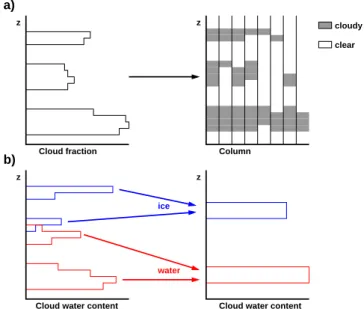
Fig. 3.Simplifications made to the cloud structure in the SEVIRI simulator:(a)each model grid cell is divided into subcolumns; in each subcolumn, a model layer that has a non-zero cloud fraction is either completely cloudy or completely clear following the stochas-tic method of R¨ais¨anen et al. (2004);(b)in each subcolumn all the ice is put into a single layer at 5–6 km, while all the liquid water is put into a single layer at 1–2 km.
as the vertical profile. For future applications that demand a more accurate representation of the model cloud reflectances, a more sophisticated value forreffwill be used (several pos-sibilities are offered by e.g. Platnick, 2000). If only a single thermodynamic phase is present in a given column, the cculations are performed for a single layer. The surface is al-ways treated as a Lambertian reflector with the albedo at the different wavelengths given by the climate model, while the clouds are assumed to be in a standard mid-latitude summer atmosphere (Anderson et al., 1986).
The simplifications of the vertical cloud structure greatly speed up the radiative transfer calculations, but come at the cost of a decrease in accuracy. The exact cost is hard to ascer-tain, but based on a sampling of a model cloud field covering Europe (see also Sect. 3.2) the error introduced is of the order of∼5 %.
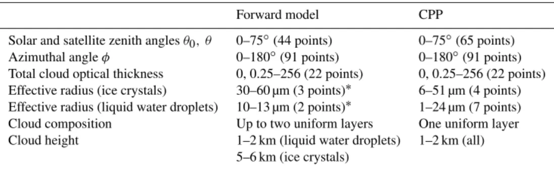
Table 1.Details of the lookup tables used in the forward model and the CPP retrieval algorithm.
Forward model CPP
Solar and satellite zenith anglesθ0, θ 0–75◦(44 points) 0–75◦(65 points) Azimuthal angleφ 0–180◦(91 points) 0–180◦(91 points) Total cloud optical thickness 0, 0.25–256 (22 points) 0, 0.25–256 (22 points) Effective radius (ice crystals) 30–60 µm (3 points)∗ 6–51 µm (4 points) Effective radius (liquid water droplets) 10–13 µm (2 points)∗ 1–24 µm (7 points) Cloud composition Up to two uniform layers One uniform layer Cloud height 1–2 km (liquid water droplets) 1–2 km (all)
5–6 km (ice crystals)
∗The effective radius values in the forward model lookup table were chosen to reflect the range in values in the RACMO climate
model.
whereas the latter does. Table 1 gives an overview of the characteristics of both lookup tables.
Once the cloud structure is simplified in this way, it can be parametrized with only four degrees of freedom: COT, optical ice fractionfice=COTice/COTtotal, andreffof both liquid water droplets and ice crystals. Together withαsurf, solar and satellite zenith anglesθ0andθand sun-satellite az-imuthal angleφ, this gives an 8-D lookup table from which the reflectances at 0.64 µm and 1.63 µm can be interpolated. This lookup table is summarised in Table 1. Interpolation is done linearly, except forαsurf, for which the equation by Chandrasekhar (1960) was used:
R(αsurf)=R(α=0)+
αsurft (θ0) t (θ ) 1−αsurfαhemi
whereRis the reflectance at the top of the atmosphere,t (θ0) andt (θ ) denote the atmospheric transmissions at solar and satellite zenith angles, and αhemi is the hemispherical sky albedo for upwelling isotropic radiation. Note that theαhemi and the productt (θ0)t (θ )are not independently given in the lookup table, but calculated from the reflectances at surface albedo 0, 0.5 and 1.
It should be noted that the choices made in the forward model, for example when it comes to ice crystal phase func-tions or 1-D versus 3-D radiative transfer calculafunc-tions, can have a profound effect on the interaction with the retrieval algorithm in a sensitivity study (cf. route III in Fig. 1). If the assumptions made in the respective codes are different, it is hard to interpret any differences in the outcome of the study as being due to inherent limitations in the retrieval algorithm.
2.2.2 Cloud physical properties retrieval algorithm
The parameters COT, reff and CWP are retrieved with the cloud physical properties algorithm (CPP) developed at the Royal Netherlands Meteorological Institute (KNMI) within the climate monitoring satellite application facility (CM SAF) of EUMETSAT (Roebeling et al., 2006). The CPP al-gorithm retrieves these properties from visible, near-infrared and infrared radiances observed by passive imagers, such as
the SEVIRI instrument onboard MSG, the Advanced Very High Resolution Radiometer (AVHRR) onboard the National Oceanic and Atmospheric Administration (NOAA) satel-lites, or the Moderate Resolution Imaging Spectroradiometer (MODIS) on board EOS Aqua or Terra.
The Nakajima and King (1990) method is used to retrieve COT and reff for cloudy pixels in an iterative manner by simultaneously comparing satellite observed reflectances at visible (0.6 µm) and near-infrared (1.6 µm) wavelengths to look-up tables (LUTs) of simulated reflectances of liquid wa-ter and ice clouds for given optical thicknesses, particle sizes and surface albedos (αsurf). The retrieval of cloud thermo-dynamic phase (ice or liquid water) is done simultaneously with the retrieval of COT and particle size. The ice phase is assigned to pixels for which the observed 0.6 and 1.6 µm re-flectances correspond to simulated rere-flectances of ice clouds, and the cloud top temperature determined from the 10.8 µm channel is lower than 265 K. The remaining cloudy pixels are considered to represent liquid water clouds (Wolters et al., 2008). Note that the retrieval of reff at low values of COT is complicated by the limited variation of the reflectance at 1.6 µm (cf. Fig. 2). For clouds with COT<8 the final value for reff is relaxed by weighting the value derived with the Nakajima and King (1990) method and a climatological av-erage value (8 µm for liquid water clouds or 26 µm for ice clouds), where the weight assigned to the climatology in-creases linearly from 0 at COT=8 to 1 at COT=0. This is done to avoid spuriously strong variations in the outcome ofreff. All clouds are assumed to be in a layer between 1 and 2 km height in a standard mid-latitude summer atmosphere taken from Anderson et al. (1986).
Assuming vertically homogeneous clouds, the CWP is computed from the retrieved COT and reff using CWP= 4/3 COT reff/Qext, whereQext is the extinction efficiency
Qext=σext/π reff2 and σext the extinction cross section of liquid water droplets or ice crystals of the appropriate size. It should be noted that Qext is almost uniformly two for droplets, so the expression simplifies to CWP=
to satellite and solar viewing zenith angles smaller than 72◦. At larger solar and viewing zenith angles the errors in the retrievals are too large due to the decreased accuracy of the radiative transfer simulations, the decreased signal to noise ratio of the reflectance observations, and the increased 3-D radiative effects (V´arnai and Marshak, 2007).
The LUTs have been generated with the Doubling Adding KNMI (DAK) radiative transfer model (Stammes, 2001). The optical thicknesses range from 0 to 256. Cloud droplets are assumed to be spherical with effective radii between 1 and 24 µm. For ice clouds, imperfect hexagonal ice crystals (Hess et al., 1998) are assumed with radii between 6 and 51 µm. Note that reff is defined slightly differently for ice crystals and liquid water droplets: for ice crystals, the vol-ume equivalent radius for a hexagonal columnrvol is used, while the radii of liquid water droplets are assumed to fol-low a gamma distribution with an effective variance of 0.15; the effective radius is defined asreff=r3/r2, withh. . .i denoting an average over the size distribution.
The MODTRAN model (Berk et al., 2000) is used to cal-culate, and correct for, the absorption by atmospheric trace gases on band-averaged reflectances as observed by satellite instruments (Meirink et al., 2009). The surface reflectance maps have been generated from five years of MODIS white-sky albedo data (Moody et al., 2008). The algorithm to sep-arate cloud free from cloud contaminated and cloud filled pixels originates from the MODIS cloud detection algorithm (Ackerman et al., 1998; Platnick et al., 2003; Frey et al., 2008). It has been modified to make it applicable to other passive imagers and to make it independent from ancillary data (Roebeling et al., 2008).
3 Results and discussion
3.1 Testing the CPP retrieval algorithm
To investigate the validity of the CPP retrieval algorithm, the simulator is used to obtain reflectances for a variety of input parameters. These reflectances are then used as input data of the CPP algorithm, and the retrieved cloud physical proper-ties are compared to the original input. The emphasis is on the retrieval of CWP, using the retrievals of COT andreff only as intermediate steps. This choice was made because CWP is a prognostic variable in climate models, while COT is usually derived from an assumedreff. Therefore, looking at retrieval errors of COT andreffis of limited relevance when the underlying purpose is to gauge the usefulness of CPP in model evaluation, and they will only be mentioned in relation to CWP retrievals.
Despite the fact that the forward model is built to calcu-late radiances from climate model output, no actual climate model data was used in the following evaluation of CPP. In-stead, the choice was made to take advantage of the com-putational speed of the forward model to sample the input
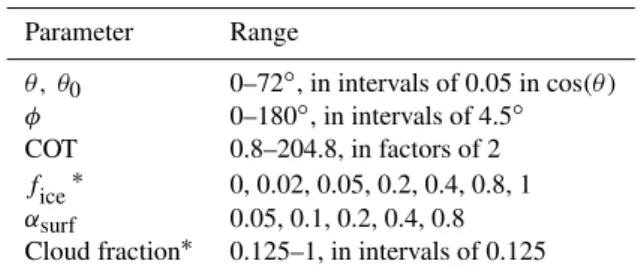
Table 2.Parameter space explored in the CPP test in Sect. 3.
Parameter Range
θ, θ0 0–72◦, in intervals of 0.05 in cos(θ )
φ 0–180◦, in intervals of 4.5◦ COT 0.8–204.8, in factors of 2
fice∗ 0, 0.02, 0.05, 0.2, 0.4, 0.8, 1
αsurf 0.05, 0.1, 0.2, 0.4, 0.8 Cloud fraction∗ 0.125–1, in intervals of 0.125
∗f
iceis only varied for clouds with cloud fraction=1; cloud fraction is
only varied for pure water clouds.
space of the simulator and perform retrievals on the resulting radiances. Thus all cloud configurations that are possible in the set-up of the forward model are studied, even unphysical ones, instead of relying on a climate model field to provide the necessary variation in clouds. The parameter space for this test is summarised in Table 2.
In the following sections, both multi-layer clouds (i.e. cloudy pixels containing both ice clouds and liquid water clouds) and clouds containing only one layer of either ice or liquid water (labeled “pure ice” and “pure liquid water”) are studied, even though the latter two cases represent ideal situations where CPP should perform optimally; in fact, the only significant source of uncertainties in this regime is the retrieval ofreff at low values of COT. The reason for this is twofold: first, the single-phase simulations provide a baseline error analysis with which other effects can be compared; for instance, retrievals ofreffbecome uncertain for low values of COT, and this will be reflected in the analysis of single-phase clouds. Second, some sources of retrieval errors such as large solar zenith angles or broken clouds become more apparent if single-phase clouds are considered because these effects can then be considered the only sources of uncertainty.
3.1.1 Effects of solar zenith angle
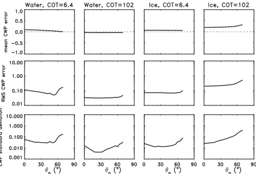
As a first test the influence on the solar zenith angleθ0on the CWP retrieval is examined for pure ice and pure liquid water clouds with a COT of either 6.4 or 102.4;αsurf was 0.1 in all cases, while the effective radii of droplets and ice crystals are kept fixed at 11 µm and 38 µm, respectively. The result-ing CWP retrieval errors, averaged over all satellite viewresult-ing angles withθ <72◦ on a grid consisting of 14 points inθ
(equidistant in cos(θ )) and 41 equidistant points in φ, are shown in Fig. 4. Three measures for the retrieval errors are used:
– the mean relative error, which indicates the bias of the retrievals, defined as(hCWPi −CWP∗)/CWP∗,
– the RMS relative error, which indicates the accuracy of the retrievals, defined asq
(CWP−CWP∗)2
Fig. 4.The CWP retrieval errors as a function of solar zenith angleθ0, for different pure liquid water and pure ice clouds (indicated at the top of each column). The top row shows the mean relative error (indicative of the bias of the retrievals); the middle row shows the RMS relative error (indicative of the accuracy of the retrievals); the lower row shows the standard deviation (indicative of the precision of the retrievals). Results were averaged over all satellite geometries withθ <72◦; the effective radii arereff=11 µm for liquid water clouds andreff=38 µm for ice clouds.
– the relative standard deviation, which indi-cates the precision of the retrievals, defined as q
(CWP− hCWPi)2
/CWP∗,
where h. . .i denotes a mean over the relevant geometries, CWP denotes the retrieved values as a function of geometry for a given cloud configuration, and CWP∗denotes the input value for this cloud configuration, which is independent of the geometry. Thus, the quantities are given as dimensionless numbers, relative to the input CWP. In all cases the errors are averaged over all satellite geometries withθ <72◦, which is the largest zenith angle where CPP can still do meaningful retrievals.
It can be seen that liquid water clouds have generally low retrieval errors in these circumstances for most solar zenith angles. This is to be expected: the conditions for the radia-tive transfer calculations used here are almost identical to those used in the CPP algorithm, except for the values of
reffand sun-satellite geometry used in the respective lookup tables; the different grids introduce slight interpolation er-rors with respect to each other. There is an additional source of errors in the retrieval of the low COT clouds; due to un-certainties in the retrieval ofreff at low optical thickness (cf. Fig. 2), CPP uses a weighted mean of the retrievedreff and a climatological mean of 8 µm for liquid water droplets and 26 µm for ice crystals. This causes a relatively low standard deviation in the retrievals, but the bias it introduces leads to RMS errors of the order of 10 %. At large solar zenith
an-gles (θ0>60◦) retrievals become more problematic and less precise as a consequence. At higher COT values this effect disappears, since it is easier to retrievereff there. The CWP retrieval errors for thin ice clouds mirror those of liquid wa-ter clouds. At large solar zenith angles, there is a predom-inantly positive retrieval error in the forward scattering di-rection, while mainly negative for backscatter. For thick ice clouds, the CWP retrieval errors are larger than for liquid wa-ter clouds. This is caused by an overestimation of COT due to a combination of two effects: first, the ice clouds in the simulator are at 6 km, while CPP assumes all clouds to be at 2 km; this causes slight differences in the Rayleigh scattering occurring above the cloud, and hence different reflectances at 0.6 µm. The second effect can be seen in Fig. 2, where the re-flectances at 0.6 µm for ice clouds saturate at a relatively low reflectance due to the small asymmetry factors of the Hess et al. (1998) ice crystals.
3.1.2 Effects of COT, multi-layer clouds and surface albedo
For a more thorough investigation of the effects of COT,
αsurfand multi-layer clouds (parametrised by the optical ice fractionfice), the reflectances are calculated for a parameter space spanning the relevant values of these parameters. This parameter space consists of a grid of 9 values of COT (rang-ing from 0.8 to 204.8), 7 values office(pure ice and pure liq-uid water clouds, plus five intermediate points ranging from
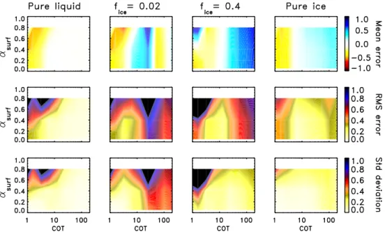
Fig. 5.The CWP retrieval errors as a function of COT andαsurf, averaged over all satellite viewing angles withθ <72◦and solar zenith angles withθ0<72◦. The columns indicate different values office, while the rows are as in Fig. 4. Again, effective radii arereff=11 µm for liquid water clouds andreff=38 µm for ice clouds.
to 0.8); for simplicity the sameαsurfvalues are used at both 0.6 and 1.6 µm. Again, the effective radii of ice crystals and liquid water droplets are taken as 38 µm and 11 µm, respec-tively, and are assumed to be uniform within the cloud.
The CWP retrieval errors are illustrated in Figs. 5 and 6. As before, the retrieval errors are averaged over all satel-lite viewing angles withθ <72◦; now they are also averaged over all solar zenith angles withθ0<72◦to focus more on the effects of the cloud and surface properties. It can be seen that retrieval errors are generally small for pure liquid water clouds, and to a lesser extent for pure ice clouds, generalising the results illustrated in Fig. 4. The only exceptions occur for low COT, caused by the aforementioned use in CPP of clima-tological mean values ofreff, and for ice clouds with an opti-cal thickness&10, caused by the fact that the simulator uses a different cloud top height from the CPP algorithm for ice clouds. As a result the COT retrievals for pure ice clouds are generally too high and quickly approach 256, the maximum COT value that CPP can retrieve. This explains the relatively high precision of the retrievals, and why the retrieval errors decrease as the input COT approaches this maximum value.
Varying the surface albedo has a limited effect on the CWP retrieval quality, increasing the uncertainties only at very high values (αsurf>0.5, i.e. snow-covered surfaces). For these bright surfaces the retrieval of COT becomes prob-lematic because the contrast between the cloud and the sur-face decreases, leading to an overestimation of COT. The un-certainties decrease for COT>10, where the surface albedo has little influence on the reflectances. For very high values of COT, the CPP algorithm tends to yield COT=256, the
maximum value in the CPP LUTs; this reinforces the rela-tively low retrieval uncertainties regardless of surface albedo as the actual COT approaches this upper limit.
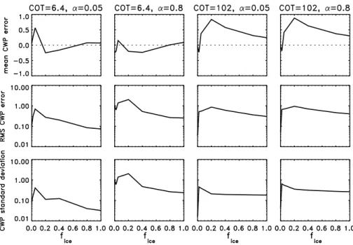
Fig. 6.As Fig. 4, except the errors are shown as functions officefor several combinations of COT andαsurf.
to a different CPP LUT, shows as a sign change in the mean error. The CWP errors in that regime are mainly caused by the mismatch between retrieved and bulk cloud values ofreff. For larger values office the errors are lower, since the re-trieved phase represents a greater part of the total cloudy col-umn.
3.1.3 Effects of fractional cloud cover
If a cloud is observed by the satellite, it will not necessar-ily fill the entire field of view. In general, a pixel that is interpreted as cloudy will have cloudy and clear parts, in-troducing uncertainties in the retrievals; specifically, reff is usually overestimated (Wolters et al., 2010; Zhang and Plat-nick, 2011) while COT and CWP are underestimated (Coak-ley et al., 2005). By construction this complication does not occur when simulating climate model fields, since the proce-dure outlined in Sect. 2.2 and Fig. 3 ensures that each sub-column used in the calculations is either completely cloudy or completely clear; yet since it may occur in the observa-tions, the uncertainties introduced when retrieving CWP for partially clouded pixels have to be assessed.
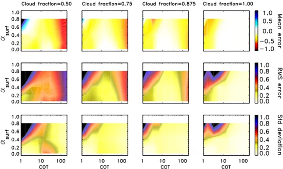
To study the effect of partial cloud cover in a pixel, the reflectances were calculated for a fully covered cloudy field and a clear sky field; a weighted mean of the results (weighted according to the required cloud cover) was then used as the reflectance of the partially cloudy field. From these reflectances the CWP retrieval error is determined. This procedure was performed for liquid water clouds with vari-ous values for COT,αsurfand cloud cover; pure liquid water clouds are chosen because they have the smallest intrinsic retrieval errors, hence the resulting errors can be considered
to be mostly due to the fractional cloud cover. The resulting CWP retrieval errors are shown in Figs. 7 and 8. It can be seen that CWP retrieval errors rise dramatically for clouds with a relatively low COT or with very high COT, even at cloud fractions of 87.5 %. Only clouds with COT=10–20 over a dark surface have low retrieval errors; for these clouds, the overestimation ofreffis found to compensate the under-estimation of COT. Retrieval errors tend to increase even fur-ther with decreasing cloud fraction, going to RMS errors of order unity for a cloud cover of 12.5 %. Retrievals of CWP are generally too low due to underestimations of COT at low
αsurf, and ofreff at highαsurf. The only exception occurs at low COT and highαsurf, where the bright surface compli-cates COT retrievals with a high chance of overestimations. It should be noted that the standard deviation of the retrievals is relatively low for cloud covers>50 %, regardless of almost any variation in COT orαsurf. Thus it is at least theoretically possible to compensate for the retrieval errors introduces by fractional cloud cover if the cloud fraction is known some-how. An exception occurs for thin clouds (COT<10) over a bright surface (αsurf>0.5), where CWP retrievals are prob-lematic in any case (cf. Fig. 5).
3.2 Application to a climate model
Fig. 7.As Fig. 5, except the results are for pure liquid water clouds, and the columns indicate different values of the cloud fraction.
Fig. 8.As Fig. 6, except the errors are shown as functions of the cloud fraction for several combinations of COT andαsurf.
modeling; it has been developed at KNMI by porting then physics package of the ECMWF IFS (European Center for Medium-Range Weather Forecast Integrated Forecasting System), release cy23r4, into the forecast component of the HIRLAM (High Resolution Limited Area Model) NWP, ver-sion 5.0.6 (de Bruijn and van Meijgaard, 2005; van Meij-gaard et al., 2008).
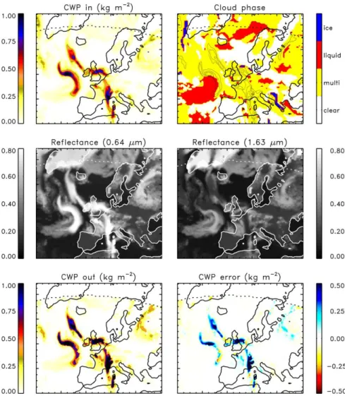
Figure 9 shows how the uncertainty analysis procedure is applied to a RACMO field across Western Europe, on 15 May 2009 at 12:00 UTC. For simplicity, the surface albedo
Fig. 9.Application of the simulator to a single RACMO field, for 15 May 2009, 12:00 UTC. The upper left panel gives the CWP calculated by RACMO; the upper right panel gives the cloud phase at each grid point (>99 % ice,>99 % liquid water, multi-layer, or clear), with countours tracing CWP for ease of reference; the center left panel gives the simulated reflectance at 0.64 µm; the center right panel gives the simulated reflectance at 1.63 µm; the lower left panel gives the retrieved CWP after the RACMO output was put through the simulator and CPP; the lower right panel gives the difference between the retrieved CWP and the RACMO CWP. In all panels the dotted line marks the area where both the solar and satellite zenith angles are less than 72◦; no retrievals are done beyond this line.
lower two panels of Fig. 9 where it is shown that nearly all clouds have their CWP overestimated by CPP. Notable ex-ceptions occur in the pure liquid water clouds north west of the Iberian peninsula. As such, large differences between SE-VIRI retrieved and model predicetd CWP can be expected in those areas, even if the climate model were a perfect repre-sentation of reality. This result also emphasises that an eval-uation of this model with satellite data should be conducted in the routes II or IV of Fig. 1, rather than route I.
3.3 Comparison with other studies
The results of this study contrast with the findings of Bugliaro et al. (2011), who performed a similar study on the retrieval errors of COT,reffand CWP. In their paper, the libRadtran 1-D radiative transfer solver was used to calculate
all the low-resolution SEVIRI channels for a single down-scaled 3-D cloud field produced by the COSMO-EU numeri-cal weather prediction model. The retrieval errors were quan-tified by comparing the cloud properties retrieved by the CPP and the APICS algorithms, both applied to the synthetic SE-VIRI reflectances, to the cloud properties in the COSMO-EU field.
mainly due to the abundance of optically thin clouds in their sample: for liquid water clouds, they have a mean COT of 9.13, so a sizeable portion of the clouds have COT values much smaller than 8. For these thin clouds, CPP will nudge itsreffretrievals towards a climatological mean of 8 µm; com-bined with a meanreffin the model field of 5.32 µm this will result in a positive bias in the CWP retrievals. In the current paper it is shown that CPP has large retrieval errors for liq-uid water clouds with COT<5, but performs well for greater optical thicknesses. The bias shown in Fig. 5 is negative due to the choice ofreff=11 µm in these calculations, but has the same origins as the positive bias in Bugliaro et al. (2011). For the thicker clouds, differences in the CWP uncertainties may also be caused by the assumptions made in each simulator and its interaction with CPP; for instance, the forward model presented here places liquid water clouds at 2 km height in a model atmosphere, as does CPP, whereas Bugliaro et al. (2011) allow for variable cloud top heights.
Another difference between the two studies occurs with the CWP retrieval of ice clouds. This is again caused by low optical depth effects; for ice clouds the mean COT is 2.15, making this effect even more pronounced than for liquid wa-ter clouds. The meanreff is 41.32 µm, meaning that the as-sumption in CPP of a climatological mean value of 26 µm for optically thin ice clouds can explain the underestimation of CWP. Also, their simulator uses different phase functions for ice crystals than CPP, while in the current paper the same type of crystals are used (albeit with different values ofreff). For multi-layer clouds the two studies agree that CWP re-trieval uncertainties are relatively large.
It is noteworthy that the APICS retrievals shown in Bugliaro et al. (2011) are generally more accurate and pre-cise than the CPP retrievals. While the present paper offers no such comparison, it should be noted that the two studies are not neutral with respect to the retrieval algorithm used. Both APICS and the forward model applied in Bugliaro et al. (2011) are based on the libRadtran radiative transfer model, while both CPP and the forward model developed here are based on the DAK code. This set-up likely influences the in-teractions bewteen the forward models and the retrieval algo-rithms, for example in the ice crystal scattering phase func-tions and the droplet size distribution.
4 Conclusions
Retrievals of cloud water path (CWP) with the CPP algo-rithm work well for pixels that are completely covered by either pure ice or pure liquid water clouds with cloud opti-cal thickness COT>5. For ice clouds, the retrieval error is within 10 % when COT<80; liquid water clouds have com-parable retrieval errors up to COT=200. A very high sur-face albedo (>0.5) leads to larger uncertainties. The CWP retrieval errors show little variation forθ0<50◦, and tend to increase for larger values ofθ0.
For multi-layer clouds, CWP retrievals become very sensi-tive to errors when there is a thin ice cloud overlying a thick liquid water cloud. With such multi-layer clouds, an accept-able retrieval of CWP can only be carried out for very low values of the optical ice fractionfice, where the ice layer is optically thin and does not interfere with the observation of the liquid water layer, and for high values of fice (>0.6), where the ice layer represents the majority of the observed cloud. These uncertainties arise from the fact that the CPP cloud phase retrievals focus on a few optical depths at the top of the cloud; in carrying out a CWP retrieval it applies this information to the whole cloud using the method outlined in Sect. 2.2.2.
When a cloud covers only part of the SEVIRI pixel, the CWP retrievals show a considerable negative bias for cloud fractions <80 %. The precision in the retrievals is quite good, however, indicating that the effects of broken cloud cover can be compensated if the cloud fraction is known somehow.
While some of the results presented here initially seem to contrast with the findings of Bugliaro et al. (2011), who per-formed a similar study, these discrepancies can be explained by differences in the experimental set-ups and assumptions that go into the respective simulators.
Acknowledgements. This work is part of the project titled “Con-struction and application of an MSG/SEVIRI simulator” that is carried out in the User Support Programme Space Research under the supervision of the Netherlands Space Office (NSO). We wish to thank Piet Stammes for the use of the DAK radiative transfer code. We would also like to thank Brent Maddux, Piet Stammes, Wouter Greuell and Jan Fokke Meirink for reviewing earlier versions of this manuscript. Further, we thank J´erˆome Ri´edi for providing the SEVIRI cloud detection code, and Olaf Tuinder for his help with technical issues.
Edited by: B. Mayer
References
Ackerman, S., Strabala, K., Menzel, W., Frey, R., Moeller, C., and Gumley, L.: Discriminating clear sky from clouds with MODIS, J. Geophys. Res., 103, 32141–32157, 1998.
Anderson, G., Clough, S., Kneizys, F., Chetwynd, J., and Shettle, E.: AFGL atmospheric constituent profiles (0–120 km), Tech. Rep. AFGL-TR-86-0110, Air Force Geophysics Laboratory, 1986.
Berk, A., Anderson, G., Acharya, P., Chetwynd, J., Bernstein, L., Shettle, E., Matthew, M., and Adler-Golden, S.: MODTRAN4 Version 2 Users Manual, Tech. Rep., Air Force Research Labo-ratory, 2000.
Bugliaro, L., Zinner, T., Keil, C., Mayer, B., Hollmann, R., Reuter, M., and Thomas, W.: Validation of cloud property retrievals with simulated satellite radiances: a case study for SEVIRI, Atmos. Chem. Phys., 11, 5603–5624, doi:10.5194/acp-11-5603-2011, 2011.
Chandrasekhar, S.: Radiative Transfer, Dover Publications, 1960. Coakley, J., Friedman, M., and Tahnk, W.: Retrieval of cloud
prop-erties for partly cloudy imager pixels, J. Atmos. Ocean. Tech., 22, 3–17, 2005.
de Bruijn, E. and van Meijgaard, E.: Verification of HIRLAM with ECMWF physics compared with HIRLAM reference ver-sions, HIRLAM Tech. Rep. 63, available from SMHI, S-601 76 Norrk¨oping, Sweden, 2005.
Donovan, D., Voors, R., van Zadelhoff, G.-J., and Acarreta, J.: EC-SIM Models and Algorithms Document, Tech. Rep., 2008. Frey, R., Ackerman, S., Liu, Y., Strabala, K., Zhang, H., Key, J., and
Wang, X.: Cloud detection with MODIS. Part I: Improvements in the MODIS Cloud Mask for Collection 5, J. Atmos. Ocean. Tech., 25, 1057–1072, 2008.
Greuell, W., van Meijgaard, E., Meirink, J., and Clerbaux, N.: Eval-uation of model predicted top-of-atmosphere radiation and cloud parameters over Africa with observations from GERB and SE-VIRI, J. Climate, 24, 4015–4036, 2011.
Hess, M., Koelemeijer, R., and Stammes, P.: Scattering matrices of imperfect hexagonal crystals, J. Quant. Spectrosc. Ra., 60, 301– 308, 1998.
Klein, S. and Jakob, C.: Validation and sensitivities of frontal clouds simulated by the ECMWF model, Month. Weather Rev., 127, 2514–2531, 1999.
Mayer, B. and Kylling, A.: Technical note: The libRadtran soft-ware package for radiative transfer calculations – description and examples of use, Atmos. Chem. Phys., 5, 1855–1877, doi:10.5194/acp-5-1855-2005, 2005.
Meirink, J., Roebeling, R., and van Meijgaard, E.: Atmospheric cor-rection for the KNMI cloud physical properties retrieval algo-rithm, Tech. Rep. TR-304, KNMI, 2009.
Molders, N., Laube, M., and Raschke, E.: Evaluation of model gen-erated cloud cover by means of satellite data, Atmos. Res., 39, 91–111, 1995.
Moody, E., King, M., Schaaf, C., and Platnick, S.: MODIS-Derived Spatially Complete Surface Albedo Products: Spatial and Tem-poral Pixel Distribution and Zonal Averages, J. Appl. Meteor. Climatol., 47, 2879–2894, 2008.
Nakajima, T. and King, M.: Determination of the Optical Thick-ness and Effective Particle Radius of Clouds from Reflected So-lar Radiation Measurements. Part 1: Theory, J. Atmos. Sci., 47, 1878–1893, 1990.
Pincus, R., McFarlane, S., and Klein, S.: Albedo bias and the hor-izontal variability of clouds in subtropical marine boundary lay-ers: Observations from ships and satellites, J. Geophys. Res., 104, 6183–6191, 1999.
Platnick, S.: Vertical photon transport in cloud remote sensing prob-lems, J. Geophys. Res., 105, 22919–22935, 2000.
Platnick, S., King, M., Ackerman, S., Menzel, W., Baum, B., Riedi, J., and Frey, R.: The MODIS cloud products: algorithms and ex-amples from Terra, IEEE T. Geosci. Remote Sens., 41, 459–473, 2003.
R¨ais¨anen, P., Barker, H., Khairoutdinov, M., Li, J., and Randall, D.: Stochastic generation of subgrid-scale cloudy columns for
large-scale models, Q. J. Roy. Meteor. Soc., 130, 2047–2067, 2004. Roebeling, R. and van Meijgaard, E.: Evaluation of the daylight
cycle of model predicted cloud amount and condensed water path over Europe with observations from MSG-SEVIRI, J. Climate, 22, 1749–1766, 2009.
Roebeling, R., Feijt, A., and Stammes, P.: Cloud property retrievals for climate monitoring: implications of differences between Spinning Enhanced Visible and Infrared Imager (SEVIRI) on METEOSAT-8 and Advanced Very High Resolution Radiome-ter (AVHRR) on NOAA-17, J. Geophys. Res., 111, D20210, doi:10.1029/2005JD006990, 2006.
Roebeling, R., Deneke, H., and Feijt, A.: Validation of cloud liquid water path retrievals from SEVIRI using one year of CLOUD-NET observations, J. Appl. Meteor. Climatol., 47, 206–222, 2008.
Rossow, W. and Garder, L.: Cloud detection using satellite measure-ments of infrared and visible radiances from ISCCP, J. Climate, 6, 2341–2369, 1993.
Rossow, W. and Schiffer, R.: Advances in understanding clouds from ISCCP, B. Am. Meteorol. Soc., 80, 2261–2287, 1999. Stammes, P.: Spectral radiance modeling in the UV-Visible range,
in: IRS 2000: current problems in atmospheric radiation, edited by: Smith, W. and Timofeyev, Y., A. Deepak Publ., Hampton, Va, 385–388, 2001.
Tselioudis, G. and Jakob, C.: Evaluation of midlatitude cloud prop-erties in a weather and a climate model: dependence on dynam-ical regime and spatial resolution, J. Geophys. Res., 107, 4781, doi:10.1029/2002JD002259, 2002.
van Meijgaard, E., van Ulft, L., van de Berg, W., Bosveld, F. C., van den Hurk, B., Lenderink, G., and Siebesma, A.: The KNMI regional atmospheric climate model RACMO version 2.1, Tech. Rep. TR-302, KNMI, 2008.
V´arnai, T. and Marshak, A.: View angle dependence of cloud optical thickness retrieved by MODIS, J. Geophys. Res., 112, D06203, doi:10.1029/2005JD006912, 2007.
Voors, R., Donovan, D., Acarreta, J., Eisinger, M., Franco, R., Lajas, D., Moyano, R., Pirondini, F., Ramos, J., and Wehr, T.: ECSIM: the simulator framework for EarthCARE, in: Proc. SPIE 6744, 2007.
Webb, M., Senior, C., Bony, S., and Morcrette, J.-J.: Combining ERBE and ISCCP data to assess clouds in the Hadley Centre, ECMWF and LMD atmospheric climate models, Clim. Dynam, 17, 905–922, 2001.
Wolters, E., Roebeling, R., and Feijt, A.: Evaluation of cloud-phase retrieval methods for SEVIRI on Meteosat-8 using ground-based lidar and cloud radar data, J. Appl. Meteor. Climatol., 47, 1723– 1738, 2008.
Wolters, E., Deneke, H., van der Hurk, B., Meirink, J., and Roe-beling, R.: Broken and inhomogeneous cloud impact on satellite cloud particle effective radius and cloud-phase retrievals, J. Geo-phys. Res., 115, D10214, doi:10.1029/2009JD012205, 2010. Zhang, Z. and Platnick, S.: An assessment of differences
be-tween cloud effective particle radius retrievals for marine water clouds from three MODIS spectral bands, J. Geophys. Res., 116, D20215, doi:10.1029/2011JD016216, 2011.